

Abstract
Despite variations in appearance we robustly recognize objects. Neuronal populations responding to objects presented under varying conditions form object manifolds and hierarchically organized visual areas are thought to untangle pixel intensities into linearly decodable object representations. However, the associated changes in the geometry of object manifolds along the cortex remain unknown. Using home cage training we showed that mice are capable of invariant object recognition. We simultaneously recorded the responses of thousands of neurons to measure the information about object identity available across the visual cortex and found that lateral visual areas LM, LI and AL carry more linearly decodable object identity information compared to other visual areas. We applied the theory of linear separability of manifolds, and found that the increase in classification capacity is associated with a decrease in the dimension and radius of the object manifold, identifying features of the population code that enable invariant object coding.
Introduction
Object recognition is an ethologically-relevant task for many animals. This is a challenging problem because an individual object can elicit myriads of images on the retina due to so-called nuisance transformations such as changes in viewing distance, projection, occlusion and illumination. The collection of neural responses associated with a single object is known as the object manifold. A prevailing hypothesis is that along the visual hierarchy, object manifolds are gradually untangled to produce increasingly invariant object representations, which are linearly decodable (DiCarlo and Cox, 2007). This hypothesis is primarily based on work in non-human primates, which is a powerful model to study object recognition especially given the similarities in visual perception among primates. These studies have revealed that the selectivity for object identity increases as visual signals are conveyed from primary visual cortex (V1) to inferotemporal cortex (Hung et al., 2005; Rust and DiCarlo, 2010). Despite this significant progress, the underlying changes in the geometry of the object manifolds along the visual cortical hierarchy that leads to object recognition and a circuit-level mechanistic understanding of how they are generated remain largely unknown. The mouse animal model is ideally suited to dissect circuit mechanisms due to its genetic tractability and the numerous methods available to perform large scale recordings, manipulations and anatomical tracing with cell-type precision (Fenno et al., 2015; Sofroniew et al., 2016). Therefore developing visually guided behaviors in rodents is important (Zoccolan et al., 2009) and identifying the relevant network of visual areas involved in object recognition analogous to the ventral stream of primates is critical. In this direction, we developed an automatic high-throughput training paradigm and demonstrated that mice can be trained to perform a two-alternative forced choice (2AFC) object classification task, which is typically used in primates to test object identification. While visually-guided operant behavioral tasks have been used previously in mice (Hu et al., 2018; Leger et al., 2013), here we show that mice can also learn to correctly discriminate objects under a 2AFC paradigm. Critically, this capability persisted even when they were presented with previously-unseen transformation of objects.
We simultaneously recorded the activity of thousands of neurons across all cortical visual areas of the mouse: primary (V1), anterolateral (AL), rostrolateral (RL), lateromedial (LM), lateral intermediate (LI), posteromedial (PM), anteromedial (AM), posterior (P), postrhinal (POR) and laterolateral anterior (LLA) visual areas, while presenting images of moving objects undergoing numerous identity-preserving transformations such as rotation, scale and translation across different illumination conditions. By decoding the identity of the objects from the recorded neural activity using a linear classifier we found that the lateral extrastriate visual areas (LM, AL, LI) carried more linearly decodable information about objects identity compared to V1 and all other higher order areas we studied, consistent with results in rats (Tafazoli et al., 2017). We used the recently developed theory of linear separability of manifolds and found that in areas LM and AL the increase in classification capacity is associated with improved manifold geometry, where both the manifold radii and dimensions are reduced compared to other visual areas. Additionally, by recording simultaneously from many visual areas, we found that the population dynamics differed across the visual hierarchy, where information about object identity accumulated faster in areas which are more object selective compared to V1.
Results
We generated rendered movies of 3D objects by varying their location, scale, 3D pose and illumination in a continuous manner across time (Fig. 1a, Supp. Movie 1). We developed a 2AFC automatic home cage training system in which water restricted mice had to lick a left or a right port depending on the object that was shown on a small monitor in front of their cage (Fig. 1b). Upon a correct choice animals immediately received a small amount of water reward. Naive animals initially licked the left and right probes at random, but within two weeks of training animals learned to preferentially lick the correct port matched to object identity (Fig. 1c) and trained animals maintained consistent performance on the task across days (Fig. 1d). An important property of object recognition is the ability to generalize across views of objects that have never been seen before. After the animals learned to discriminate objects from the movie clips - which contained a specific set of object transformations, new movie clips with unique parameters across translation, scale, pose and illumination, were presented to the animals. We could not detect any differences in performance between the previously seen object transformations (Fig.1e, familiar transformations) and novel object transformations (Fig.1e, novel transformations). This ability to generalize across identity-preserving transformations indicated that mice learned an internal object-based model and did not rely simply on low-level features of the rendered movies they observed during training.

(a) Single frames from movies with the objects that were presented to the animals. (b) Behavioral training sequence. (c) Probability of licking either probe during the early training period (upper barplot) and later training period (lower barplot) for 1 animal. Error bars represent S.E.M. Student t-test * p < 0.05 (d) Performance as a function of training time, N = 8 animals. (e) Performance across repetitions of previously seen (gray) and previously unseen (red) object trajectories during one session. N = 6 animals. For both (d) and (e) shaded areas represent S.E.M. (f) Example large field of view recording (green) with area boundaries overlaid. Scale bar represents 1mm. A small inset depicts the two-photon average image for a small segment of the large field of view captured with the mesoscope. (g) Example responses of all neurons to moving objects (shown on top) from the recording shown in (f). Each clip is presented for 3-5 seconds before a short pause switches to a new clip that might be the same or a different object identity.
If mice were capable of discriminating between objects, there should exist a set of areas along their visual processing hierarchy that can extract this information. It has been suggested that one way of extracting the object information irrespective of its transformations is to have neural representations for each object that are untangled, i.e. can be read-out using a linear decoder (DiCarlo and Cox, 2007). To test this idea, we used transgenic mice expressing GCamp6 in pyramidal neurons and recorded the activity from hundreds of neurons in each visual areas separately or from thousands of neurons across the whole visual cortical hierarchy of the mouse using a large field of view microscope (Sofroniew et al., 2016, Fig. 1f, g), while the animals passively viewed the moving objects (Fig. 1a). We identified the borders between visual areas using wide-field retinotopic mapping as previously described (Fahey et al., 2019; Garrett et al., 2014; Wang and Burkhalter, 2007) (Fig. 1f). Neurons in all of the identified visual areas showed significantly more reliable responses when compared to neurons that were not assigned to any visual area, based on the area segmentation (Supp. Fig. 1a).
To measure how linearly discriminable the responses to the different objects were, we used cross-validated logistic regression to classify the object identity from the responses of neurons in each visual area. As expected, discriminability increased as a function of the number of neurons sampled (Fig. 2a), but only the higher visual areas, LM, LI and AL, showed consistently higher discriminability levels compared to V1 responses (Fig. 2a, b, c). In contrast, areas RL, AM, P, POR and LLA had significantly lower discriminability levels when compared to V1 (Fig. 2b). The differences in decoding between these areas persisted at the single neuron as well (Fig. 2d, Supp. Fig. 2a).

(a) Discriminability of object identity as a function of the number of neurons sampled. Each line represents the average across all recorded sites. (b) Scatter plot of the discriminability of different areas with a 64 population of neurons compared to V1 for all the recording sites. Insert histogram represents the difference between the discriminability of each area and V1. Red line and number indicate the mean difference. Diamonds represent the results with 2 objects whereas circles represent the results with 4 objects. Outliers have been omitted for better visualization. Wilcoxon signed rank test *** p < 0.001, ** p <0.01, * p < 0.05. (c) Average discriminability of all visual areas with a 128 population of neurons. The number below each area represents the recording sites sampled. (d) Same as in (c) but when using a single neuron at a time to decode the object identity. The number below each area represents the cells sampled. (e) Low-dimensional representation of the 128-dimensional neural activity space, illustrating the separation of the responses to four different objects for three example areas. Each dot represents the average of the activity in one 500msec bin. The side histograms represent the distances of the data projected onto each of the four object category axes for the same-class (colored) and different-class (gray). Each insert represents the confusion matrix after decoding.
We performed several control analyses: first, our results might be due to differences in the retinotopic coverage across areas. As has been reported before (Garrett et al., 2014), the coverage of the visual field is different between visual areas. To control for this, in some experiments we also mapped the receptive fields (RFs) of all recorded neurons using a dot stimulus (see methods) and repeated our decoding analysis using only neurons from each area with RF centers within the same ∼20 degree area of visual space. When we restricted our analysis in this way, areas LM, LI and AL still showed significantly higher discriminability (Supp. Fig. 2b). Another potential confound might be differences in receptive field sizes across areas (Murgas et al., 2020; Wang and Burkhalter, 2007). An area with larger receptive fields might be better at representing objects simply because more neurons are responding to the object at any moment. Indeed, when we examined decoding performance conditioned on the object size, we observed an increase in discriminability for all visual areas as a function of object size (Supp. Fig. 3a), in agreement with the increased performance we found when sampling from more neurons (Fig. 2a). However, if changes in receptive field size alone result in an increase in object discriminability we would expect that area PM that has very large receptive fields (Murgas et al., 2020) would also have high object discriminability which was not the case in our data (Fig. 2). To further investigate the influence of receptive field size on discriminability, we modeled the effect of changing receptive field (RF) size in a simulated population of neurons with filters learned by a sparse coding model. Increasing the size of the receptive fields by either scaling or pairwise linearly combining them (Supp. Fig. 4a, see Methods) led to either a decrease in discriminability or had no significant effect respectively (Supp. Fig. 4b). These results argue that our in vivo results cannot be trivially explained by differences in the receptive field sizes across visual areas. Additionally, higher visual areas have been reported to have different temporal frequency selectivities (Andermann et al., 2011; Han et al., 2018; Marshel et al., 2011). To determine whether the range of speeds that objects were moving in the movies that we showed influenced our results, we computed the decoding performance for each area as a function of the object speed, but did not find any significant differences (Supp. Fig. 3b). Therefore, we interpret the increase in discriminability in AL, LI, and LM indicating that these visual areas are specialized for the processing of visual object information with neural representations that are easier to decode (Fig. 2e).
An important property of visual areas that extract information about object identity is robustness to background clutter in the visual scene. To assess the effect of background-clutter, we first trained a logistic regression decoder on responses to objects with a gray background as we used previously. We then evaluated the performance of the decoder on the responses to movies in which we embedded the objects on top of background clutter (Fig. 3a, Supp. Movie 2). While the discriminability decreased for all visual areas when compared to noise-free stimuli (Fig. 3b), areas LM and AL maintained significantly higher discriminability compared to V1 and all other visual areas (Fig. 3a,b,c), indicating that in addition to being highly invariant to changes in the appearance of the object, the object representation in these areas is also more robust than in V1 and other visual areas to clutter. We also studied the relationship between discriminability and reliability of the neural responses. Although the decoding performance of the objects without the background correlated well with the reliability of the responses for both V1 and the lateral visual areas, when background noise was introduced this relationship broke down for V1 but not for the lateral visual areas Supp. Fig. 1b).
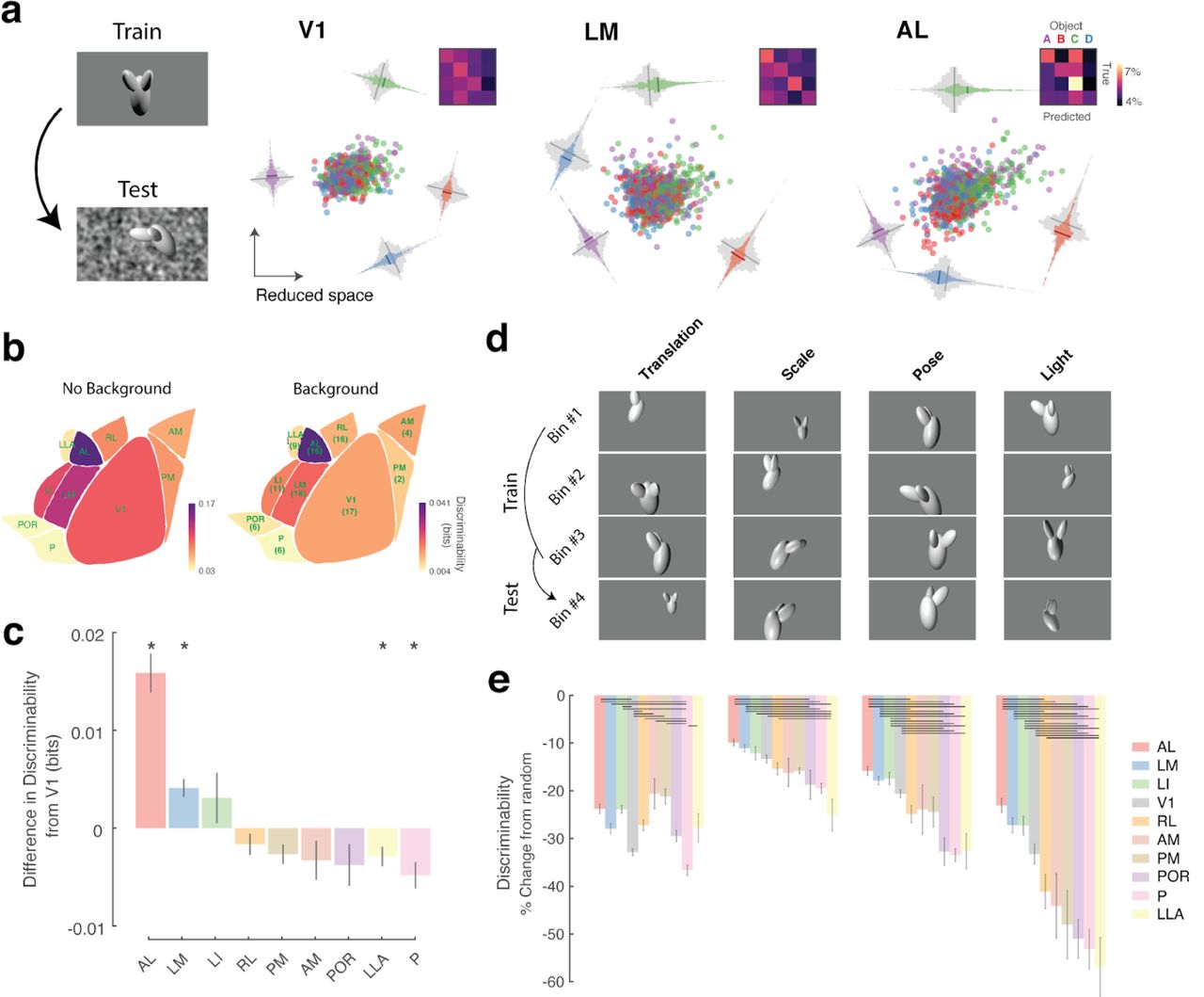
(a) Generalization test across background noise. The decoder was trained on the responses to objects without background and tested on the responses to objects that contained background noise. Low-dimensional representation of the responses to the object w/ background are shown on the right similar to Figure 2e. Each insert represents the confusion matrix after decoding. (b) Average discriminability of all visual areas for objects w/o and w/ background, on the same recorded sites. (c) Barplot indicating the difference in discriminability between all visual areas and V1 on the responses to objects w/ background. Kruskal-Wallis with multiple comparisons test *p < 0.001. (d) Example parameter space of the four nuisance classes: Translation (x/y), Scale, Pose (tilt/rotation) and Light (four light sources). The decoder was tested on a parameter space of each of the four nuisance variables that had not been part of the training set. (e) Bar plot indicating the performance when testing on untrained parameter space, compared to the performance of the random sampling across all classes. Lines indicate p < 0.05 Kruskal-Wallis with multiple comparisons test.
Neurons in an area that is specialized for representing objects should depend less on object parameters that preserve the identity such as position, scale, pose and illumination conditions (DiCarlo and Cox, 2007; Hénaff et al., 2019; Rust and DiCarlo, 2010; Tafazoli et al., 2017). As a result, an object decoder built on a subset of the nuisance parameter space (for example a limited range of translations, sizes, and rotations) should generalize across nuisance parameters. To test this we split the data into four non-overlapping bins for each of the nine continuously-varying parameters that defined the object stimulus (for example for the size object parameter, very small, small, medium, and large objects; Fig. 3d), while the remaining parameters were randomly sampled. For each parameter, we then used data from three of the bins to train the decoder, and tested the prediction performance on the held-out bin of the data. We compared this performance to a baseline discriminability using a 4-fold cross validation, when the values for each parameter were randomized before binning so that the training and test set both spanned the same parameter range. Comparing the out-of-training set performance to this baseline allowed us to assess the ability of the decoder to generalize, and thus assess the invariance of the representation in each area (Supp. Fig. 5, Fig. 3e; negative values). Areas AL, LM and LI consistently showed the best generalization performance (smallest reduction in performance for out-of-training-set condition vs baseline), when changing the scale, pose, light but not translation (Fig. 3e). The larger receptive field sizes of areas PM and AM (Murgas et al., 2020; Wang and Burkhalter, 2007) might contribute to the improved translation invariance that we observed relative to the other parameters.
Chung and colleagues (Chung et al.,2018) recently developed the theory of linear separability of manifolds and defined a measure called the classification capacity which quantifies how well a neural population supports object classification. The classification capacity measures the ratio between the number of objects and the size of the neuronal population that is required for reliable binary classification of the objects, and is tightly related to the geometry of a neuronal population responding to an object presented under varying conditions (object manifold). In deep neural networks trained on object classification tasks, it has been shown that the classification capacity improves along the network’s processing stages (Cohen et al., 2020). Our data, consisting of responses of large neuronal populations in different visual areas to objects under various transformations, are well suited for applying this method to characterize the object manifolds in different visual areas. We used the neuronal responses of 64 simultaneously recorded neurons from each visual area to four objects under the identity-preserving transformations introduced earlier (object position, scale, pose and illumination conditions, with and without background noise). In agreement with our decoding results, we found that the classification capacity increased in higher visual areas AL and LM compared to V1, but decreased in the rest of the areas (Fig. 4a,b). The theory of linear separability of manifolds (Chung et al., 2018) also enabled us to characterize the associated changes in the geometry of the object manifolds to understand how object invariant representations arise along a processing hierarchy (Cohen et al., 2020) (i.e. relate the manifolds’ classification ability to the geometry of object manifolds). In particular, classification capacity depends on the overall extent of variability across the encoding dimensions, the radius of the manifold, but also the number of directions in which this variability is spread, the dimension of the manifold. These geometric measures influence the ability to linearly separate the manifolds (Fig. 4c). In our results, we find that the increase in classification capacity can be traced to changes in the manifolds’ geometry, both as a decrease of the dimension and radius of object manifolds (Fig. 4d).
One question that arises is how these visual areas are able to form invariant representations that can generalize across background noise or nuisance parameters. One way for these areas to optimize the representations is by taking advantage of the temporal continuity that exists for natural objects by integrating information over time (DiCarlo et al., 2012; Orlov and Zohary, 2018). We analyzed the temporal dynamics of the decoding performance of 50 simultaneously recorded neurons for objects overlaid on background noise. From one trial to the next the nuisance parameters varied continously but the object identity was preserved (cis trials) or switched (trans trials) (Fig. 1g). When we compared the discriminability as a function of time for cis/trans trials, we found that indeed in the trials in which the identity of the object was switched (trans trials), discriminability was overall lower across all visual areas in the early phase of the trials compared to the late phase of the trials, providing evidence for temporal integration during a trial (Supp. Fig. 6). In the late period discriminability in area AL was significantly closer to the discriminability levels of the cis trials than all the rest of the visual areas, suggesting that activity in AL more quickly evolved to more disentangled representations (Supp. Fig. 6b, Early/Late).

(a) Scatter plot of the classification capacity of different areas compared to V1 for 4 objects. Insert histogram represents the difference between the classification capacity of each area and V1. Red line and number indicate the mean difference. Wilcoxon signed rank test *** p < 0.001, ** p <0.01, * p < 0.05. (b) Average classification capacity of all visual areas with a 64 population of neurons. The number below each area represents the recording sites sampled. (c) Illustration of low dimensional representations of object manifolds for two visual areas. Left: each point in an object manifold corresponds to neural responses to an object under certain identity-preserving transformations. Right: demonstration of two possible changes in the manifold geometry in a higher order area, reduction of the radius of one manifold through reduction of its extent in all directions (top) and reduction of the dimension of one manifold by concentrating variability at certain elongated axis, reducing the spread along other axes. Such changes have predictable effects on the ability to perform linear classification of those objects. (d) Box plots of the manifold radius (left), and manifold dimension (right) of all areas, sorted in ascending order of the median value.
A natural question is what are the dependencies between the representations of objects across multiple visual areas. If information about object identity propagates across areas, then we expect to see consistent temporal relationships in the evolution of object discriminability across these areas. We estimated each area’s confidence about the identity of the object at each time point, as the distance of the population activity from the decision boundary (Fig. 5a), and we examined the evolution of this metric across time in each area. Specifically, we estimated the distance to the decision boundary at different moments within the trial for the class that was presented. This decision boundary was a linear hyperplane in the 128 dimensional neural activity space (Fig. 5a). We then computed the correlation between the resulting temporal vectors of the score values across all simultaneously recorded visual areas (Fig. 5b, Score Correlation). The highest correlations in this moment-to-moment discriminability score were between AL, LM, RL and V1 (Fig. 5c).

(a) Schematic representation of the classification scores as the distances of the response trajectories to the decision boundary (left) and their resulting temporal dependencies across different areas (right). (b) Score correlations across all recorded areas (left) and raw pairwise correlations of the single neuron activity between areas (right). Significance was estimated by bootstrapping across all correlations, *p < 0.025/45. (c) Schematic representation of the score partial correlation coefficients between areas.
Given that activities of neurons across areas can co-fluctuate because of global brain states, these score correlations could just be the result of raw activity correlations across areas. To test this we computed the activity correlations between the responses of pairs of neurons across visual areas. We observed a different correlation pattern that was distinct from the structure of the score correlation (Fig. 5b, Score correlations vs Pairwise activity correlations). Additionally, there are multiple dependencies that can affect the score correlation between the activity of pairs of areas. In order to measure the strength of the linear relationship between each pair of areas after adjusting for relationships with the rest of the areas, we computed the partial score correlations. The correlation pattern remained unchanged with strong dependencies between V1-LM, V1-RL and LM-AL suggesting that these areas work together as a network of areas specialized for object recognition (Fig. 5c). Interestingly, we did not find a strong relationship between V1-AL (Fig. 5c).
Discussion
The ability to recognize, discriminate, and track objects across time is evidently a key adaptive trait that is fundamental to identifying food items or conspecifics (Jones and Ratterman, 2009) and the ability to recognize objects has been observed not only in higher mammals such as humans and monkeys, but also rodents, birds, fish and insects (Bevins and Besheer, 2006; Blaser and Heyser, 2015; Newport et al., 2018; Soto and Wasserman, 2014; Werner et al., 2016; Zoccolan et al., 2009). While the implementation of how information is extracted from the visual scene may vary across species, the computational problem remains the same: construct an invariant representation of objects under a wide range of identity-preserving transformations. While there is plenty of evidence that mice can detect novel objects (Leger et al., 2013), and that mice rely on their vision to hunt crickets (Hoy et al., 2016), until our study there was no direct evidence that mice are capable of invariant object recognition.
In this work, we showed that mice can be trained to recognize unfamiliar objects in a 2AFC paradigm (Fig. 1). Similar tasks have been developed for rats (Zoccolan et al., 2009), but mice have not been reported to perform such a task. That might be related to the fact that even though mice and rats can achieve similar performance levels, mice are slower to train (Jaramillo and Zador, 2014). Our unique training approach involves minimal interactions with the animals since the training system is part of their housing. Within a few weeks animals learn to discriminate objects and can show generalization across unseen objects poses establishing that mice are capable of invariant object recognition (Fig. 1d).
To identify how animals are able to extract object identity, we analyzed the activity of thousands of neurons of all known visual cortical areas of the mouse. We found that the decoding performance varied across the visual hierarchy. A set of lateral visual areas carried more linearly decodable information about the object identity. Importantly, these areas retain the information about object identity even in difficult visual conditions such as clutter and generalization across nuisance variability. Our results agree with the hypothesis that object representations become untangled and more linearly separable as information progresses through the visual hierarchy; this process might be beneficial as a simple readout mechanism may be employed in order to use this information to drive behavior. It is important to note that a biologically plausible readout mechanism would involve sampling only from a small set of neurons in order to extract object identity and that was our motivation in restricting the access of the decoder to a small sample of neurons. Interestingly, when computing the information per neuron we find that information also increased progressively across the lateral hierarchy of V1-LM-LI as has been reported in electrophysiology studies in the rat (Tafazoli et al., 2017) (Supp. Fig. 2a). However, we found that for larger populations area LI carries less information than LM (Fig. 2a, b). This could be due to more redundant information between neurons in LI in the responses to the specific set of objects used in this study. Therefore, analogous to primates in mice hierarchically organized visual areas untangle pixel intensities into more linearly decodable object representations.
However, the associated changes in the geometry of the object manifold along the visual cortex remain unknown for any species. To that end, we characterized how the geometry of the object manifolds changed across the visual hierarchy, using the newly developed theory of linear separability of manifolds (Chung et al., 2018; Cohen et al., 2020). We found that the two lateral visual areas LM and AL showed increased classification capacity with manifolds that become smaller and have lower dimensionality (Fig. 4). While the classification capacity and radius of object manifolds has not been previously quantified along the visual processing hierarchy, our results on the dimensionality of the neural population agree with previous work. Different methods have been used to quantify the dimensionality of the population responses which also showed that it decreases along the visual hierarchy of monkeys (Brincat et al., 2018; Lehky et al., 2014). However, critically the theory of the linear separability of manifolds differs from these previous methods as it quantifies the geometrical properties of the object response manifolds which contribute to the ability to perform linear decoding and thus enabled us to determine how the object manifold changes from primary to higher visual areas in a way which allows for linear decoding of objects using smaller number of neurons.
The higher visual areas of the mouse (Glickfeld and Olsen, 2017; Wang and Burkhalter, 2007), have distinct spatio-temporal selectivities (Andermann et al., 2011; Marshel et al., 2011) and project to different targets (Wang et al., 2012). Based on these differences in their selectivities, projection and chemoarchitectonic patterns, efforts have been made to separate areas into ventral and dorsal pathways analogous to those described in primates (Smith et al., 2017; Wang et al., 2012, 2011; Wang and Burkhalter, 2013). Specifically, areas such as LM, LI, P and POR areas are hypothesized to comprise the ventral stream whereas areas AL, RL, AM and PM comprise the dorsal stream. In rats, lateral visual areas LM, LI and LL have been shown to carry progressively more information about objects (Tafazoli et al., 2017; Vermaercke et al., 2015, 2014). However, the areas of the mouse that might be involved in extraction of object information are not known. We found that higher visual areas AL, LM and LI had significantly more information about object identity than V1, with area AL consistently outperforming all other areas which is not consistent with the current assumption that AL is part of the dorsal pathway. In line with this, both areas AL and LM show faster accumulation of information about object identity in noisy conditions (Supp. Fig. 6). Moreover, the correlations in decoding confidence between areas AL and LM we find (Fig. 5c) could be the result of recurrent processes that have been suggested to play a significant role during object recognition (Kar et al., 2019; Tang et al., 2018, 2014). These object-selective dependencies do not share the same structure as have been reported with more parametric stimuli (Smith et al., 2017), which could be due to objects having a statistical structure closer to the preferences of these lateral visual areas.
Future experiments are required to determine how these different areas work together to extract information about objects that might be used to guide behavior. In order to establish a more causal relationship between visual areas and behavior, it will be important to combine behavioral performance with neural activity manipulation. Neural networks models and the inception loop methodology will enable the characterization of the specific features that drive neurons in these different visual areas (Bashivan et al., 2019; Ponce et al., 2019; Walker et al., 2019).
In summary, we offer evidence that mice share similarities with rats and higher mammals in their ability to recognize objects. We show that sequential visual processing leads to object manifolds with decreased radius and dimension such that the manifolds are more linearly separable. Given the panoply of tools available, the mouse has the potential to become a powerful model to dissect the circuit mechanisms of object recognition.
Methods
Animal preparation and two photon imaging
All procedures were approved by the Institutional Animal Care and Use Committee (IACUC) of Baylor College of Medicine. We used 25 adult mice expressing GCaMP6s in excitatory neurons via either SLC17a7-Cre, Dlx5-Cre, Ai75, Ai148, Ai162 or CamKII-tTA transgenic lines. Animals were initially anesthetized with Isoflurane (2%) and a 4∼mm craniotomy was made over the right visual cortex as previously described (Froudarakis et al., 2014). The animals were head-mounted above a cylindrical treadmill and calcium imaging was performed using Chameleon Ti-Sapphire laser (Coherent) tuned to 920 nm. We recorded calcium traces by using either a large field of view mesoscope (Sofroniew et al., 2016) equipped with a custom objective (0.6 NA, 21mm focal length) with a typical field of view of ∼2500×2000μm, or a two-photon resonant microscope (Thorlabs) equipped with a Nikon objective (1.1 NA, 25X) with a typical field of view or ∼500×500μm. Laser power after the objective was kept below ∼60mW. We recorded data from depths of 100–380 μm below the cortical surface. Imaging was performed at approximately 5-12∼Hz for all scans. Imaging data were motion corrected, automatically segmented and deconvolved using the CNMF algorithm (Pnevmatikakis et al., 2016); cells were further selected by a classifier trained to detect somata based on the segmented cell masks.
Behavioral training
The mice are trained in a 2 alternative forced choice task in response to moving objects that are presented on a small 7” monitor that is located in front of their home cage. The training procedure is illustrated in Figure 1. Briefly, naive water unrestricted mice are placed in a modified cage that has three ports and a monitor on one side of the box. The center port has a proximity sensor, and the two other ports on either side of the central port are used to detect licks and are coupled to a computerized valve-controlled liquid delivery that can deliver liquid volumes with 1uL resolution. The task is as follows: Mice initiate a trial by placing their snout in close proximity to the central port for ∼200-500msec. A stimulus that can be one of two objects is presented on the monitor that is ∼1.5” in front of the animal. The animal has to report the identity of the object by licking one of the side ports. Each port is allocated to the identity of the same object throughout the training. If the animal licks the correct port, then a small water reward ∼5-12µl is delivered almost immediately which the animals consume. A new trial can be started thereafter. If the animal licks the wrong port, a short delay 4-10 seconds is added and the screen turns black. A new trial can start after the delay. Animals have free access to food, and the only water that they receive comes from their training. The training periods in which animals can initiate tasks are restricted to 4-8 hours a day. At the start of the training animals are shown the same clip for each object that contains the same set of transformations. Once animals reach performance levels, new clips with unique transformations are added. At the end of their training they have seen between 10-20 unique 10s clips of unique object transformations. For the generalization test, at the start of a new session a whole new set of 10 clips are used for each object and the performance was compared to the session that preceded.
Visual area identification
We generated retinotopic maps of all the visual areas using widefield imaging. The signals from GCamp6s were captured using either a custom epifluorescence setup or two-photon imaging. For the epifluorescence, brain was illuminated with a high power LED (Thorlabs) and the emitted signal was bandpass filtered at nm and captured at a rate of 10 Hz with a CMOS camera (MV1-D1312-160-CL, PhotonFocus). For the two-photon retinotopic mapping we sampled the activity from a 2.4⨯2.4mm area with large field of view two photon microscope (Sofroniew et al., 2016) at a rate of ∼5Hz. We stimulated with upward and rightward drifting white bars (speed: 9-18deg/sec, width: 10-20deg) on black background that had their size and speed constant relative to the mouse perspective as previously described. Additionally, within the bar we had drifting gratings with a direction opposite to the movement of the bar. Images from either the epifluorescent or the two-photon setups were analyzed by a custom-written code in MATLAB to construct the 2D phase maps for the two directions. We used the resulting retinotopic maps to identify the borders and delineate the visual areas as previously described (Garrett et al., 2014; Wang and Burkhalter, 2007).
Stimulus generation and visual stimulation
In this study we used four synthesized three-dimensional objects that were rendered in Blender (www.blender.org). Two of the objects were built to match the objects used in (Zoccolan et al., 2009) and the other two were already existing models within Blender. We varied the following parameters of the objects: X and Y location (Translation), magnification (Scale), tilt and axial rotation (Pose) and variation of either the location or energy of 4 light sources (Light). The different object parameters were varied continuously over time in order to generate a cohesive object motion. Objects were rendered either on a gray background, or on a gaussian noise pattern with a fixed seed between objects. The long rendered movie was split into smaller 10 second clips. A short 3-5 second segment from 150-380 clips for each object were presented in a random sequence to the left eye with a 25’’ LCD monitor positioned ∼15cm away from the animal. A small number of clips were repeated multiple times in order to estimate the reliability of the neural responses.
Decoding and discriminability
We used a one-versus-all logistic regression classifier to estimate the decoding error between the neural representations of 2-4 objects of 200-500 ms scenes. Each scene was represented as an N-dimensional vector of neural activity for each response scene. In almost all of the cases we used a 10 fold cross-validation in which the performance of the decoder was tested on 10% of the data that were held out during training. When generalizing across the background noise in Figure 3, the decoder was trained on 90% of the data with the no-background objects and tested on 10% of the data with the background objects. For the generalization across object parameters in Figure 3 we used a 4 fold cross-validation in which the decoder was trained on 75% of the data, and tested on 25% with a unique parameter range. We converted the decoding error to discriminability, the mutual information (measured in bits) between the true class label c and its estimate, by computing
 where pij is the probability of observing true class i and predicted class j and pi. and p.j denote the respective marginal probabilities.
Classification capacity and geometry of manifolds
An object manifold is defined by the neuronal population responses to an object under different conditions (i.e. identity-preserving transformations). The ability of a downstream neuron to perform linear classification of object manifolds depends on the number of objects, denoted P, and the number of neurons participating in the representation, denoted N. Classification capacity denotes the critical ratio αc = P /Nc where Nc is the population size required for a binary classification of P manifolds to succeed with high probability (Chung et al., 2018). This capacity can be interpreted as the amount of information about object identity coded per neuron in the given population. Capacity αc depends on the radius of each of the manifolds, denoted RM, representing the overall extent of variability (relative to the distance between manifolds), and their dimension, denoted DM, representing the number of directions in which this variability is spread. These geometric measures are defined through the alignment of the hyperplane in the representation N-dimensional space that separates positively labelled from negatively labelled manifolds. This hyperplane is uniquely determined by a set of anchor points, one from each manifold, that lie exactly on the separating plane. As the classification labels are randomly changed, the identity of the anchor points change, and these changes in addition to the dependence of the hyperplane orientation on the particular position and orientation of the manifolds, give rise to a statistical distribution of anchor points. Averaging the extent and directional spread of the anchor points with this distribution determines the manifolds radii and dimensions, respectively. Knowledge of manifold radius and dimension is sufficient to predict classification capacity using the relation αc = αBalls(RM, DM) where αBalls is a closed-form expression describing capacity of D -dimensional balls of radius R (Chung et al., 2018).
The separability of manifolds depends not only on their geometries but also on their correlations. For manifold classification with random binary labeling, clustering of the manifolds in the representational space, as expected for real-world object representations, hinders their separability, and the theory of manifold classification has been extended (Cohen et al., 2020) to take these correlations into account in evaluating αc. Here we used the methods and code from (Cohen et al., 2020) to analyze the geometry of the object manifolds (i.e. manifold radius and dimension) as well as estimate classification capacity of neuronal populations in the different cortical areas. As those methods depend on the correlation structure of the objects, we analyzed neural representations for data-sets of 4 objects (i.e. omitted data-sets where only 2 objects are available). At each session of simultaneously recorded neurons we have sub-sampled from the available population 64 neurons; the subsequent analysis was repeated 10 times with different choices of neurons, and we report the average results across this procedure. Each object manifold is defined by neural responses to an object at non-overlapping 500ms time windows, using the entire range of nuisance parameter space, as well as responses with and without background noise. This analysis was performed at each visual area for sessions where more than 64 neurons are available. The baseline to which classification capacity is compared is the value expected by structure-less manifold which is 2/M, where M is the number of samples.


