

Abstract
The dimensionality of a network’s collective activity is the number of modes into which it is organized. This quantity is of great interest in neural coding: small dimensionality suggests a compressed neural code and possibly high robustness and generalizability, while high dimensionality suggests expansion of input features to enable flexible downstream computation. Here, for recurrent neural circuits operating in the ubiquitous balanced regime, we show how dimensionality arises mechanistically via perhaps the most basic property of neural circuits: a single number characterizing the net strength of their connectivity. Our results combine novel theoretical approaches with new analyses of high-density neuropixels recordings and high-throughput synaptic physiology datasets. The analysis of electrophysiological recordings identifies bounds on the dimensionality of neural responses across brain regions, showing that it is on the order of hundreds – striking a balance between high and low-dimensional codes. Furthermore, focusing on the visual stream, we show that dimensionality expands from primary to deeper visual areas and similarly within an area from layer 2/3 to layer 5. We interpret these results via a novel theoretical result which links dimensionality to a single measure of net connectivity strength. This requires calculations that extend beyond traditional mean-field approaches to neural networks. Our result suggests that areas across the brain operate in a strongly coupled regime where dimensionality is under sensitive control by net connectivity strength; moreover, we show how this net connectivity strength is regulated by local connectivity features, or synaptic motifs. This enables us to interpret changes in dimensionality in terms of changes in coupling among pairs and triplets of neurons. Analysis of large-scale synaptic physiology datasets from both mouse and human cortex then reveal the presence of synaptic coupling motifs capable of substantially regulating this dimensionality.
Introduction
Recurrent circuits implement important network functions such as amplification, pattern completion (1–4), dimensionality reduction and feature expansion (5–7), facilitating decoding, categorization (8), and other computations. The connectivity of these circuits has been quantified in both theoretical (9–14) and experimental studies (15–18) in terms of synaptic motifs between pairs or triplets of neurons. Several studies have highlighted the potential function of these synaptic motifs for stabilizing encoded signals (19), gating circuits (20) and memory formation (14, 21). This mechanistic approach investigates how network computation arises from local connectivity structures that are the blocks of neural circuits.
A complementary approach to studying network computation is to analyze the statistical properties of the neural activity. Prominent examples characterize the variability of neural population responses in terms of average correlations (22–24), dimensionality (25–28), recurrency (29) and other statistical features (30, 31). These studies investigate the signatures of network computation in measurable features of neural activity.
Here we develop new theoretical tools that bridge these mechanistic and statistical approaches. We show that a single number measuring the effective network connectivity at a given activity level, the spectral radius, is determined by local synaptic motifs and regulates not only the degree of criticality of network dynamics (32), but also the most basic aspect of their statistics: their dimensionality. Previous theoretical contributions linked average connectivity (33–37), the block and spatial structure of connectivity (38–42) or connectivity motifs (10, 11, 43–49) to activity correlations, linked connectivity length and timescales (50) or low-rank structures (51) to low-dimensional activity patterns or linked general motifs and other network structures (5) to the spectral density of neural activity, emphasizing the consequence of reciprocal motifs for the dimension of network activity (52) (cf. Suppl. Notes). Here we develop a novel closed-form expression that directly links all second-order network motifs to a single, overall measure of recurrent coupling strength. This provides, in turn, a new direct link between network motifs and activity dimension in balanced networks, which allows us to understand the role of local synaptic motifs in modulating global network responses, and to show how their sensitivity to local motifs arises in the strong coupling regime.
We apply our theory linking connectivity and dimensionality to large scale electrophysiology recordings (53, 54) using neuropixel probes to record from more than 30000 neurons. First, we show that these recordings display the key signatures of the strong coupling regime in which our theory predicts that dimensionality is sensitivity regulated by connectivity. We then identify two important trends: dimensionality expands from primary to deeper visual areas and similarly within an area from layer 2/3 to layer 5. Finally, we analyze an allied synaptic physiology dataset in which synaptic connections among more than 22000 pairs of neurons were probed (55). This allows us to validate the involvement of local circuit motifs in modulating the dimensionality across cortical layers.
Our results were previously reported in abstract form (56).
Electrophysiology recordings display signatures of strongly recurrent dynamics across brain areas
Do brain networks operate in a strongly recurrent regime? Recent theoretical work has developed a robust way to assess the strength of recurrent coupling based on activity measurements from neural circuits (32). We start by using this method, previously applied only to a single brain area (macaque motor cortex), to analyze large-scale neural activity data recorded across multiple regions of the mouse brain. These data were recorded by the Allen Institute for Brain Science using recently developed, very high density neuropixel probes, Fig. 1a, and are freely and publicly available together with software and online visualization tools (for details see (53, 54)). We analyzed 32043 neurons across 15 brain areas (Table S1), recorded during sessions lasting on average more than 3 hours (cf. sample of 2 minutes of recorded activity, Fig. 1b). We focused on periods where either no stimulus was presented to the animal (spontaneous condition) or where drifting gratings were displayed (evoked condition, cf. Methods), Fig. S1.

a) Example of screen displayed to the animal during the evoked condition (where the stimulus presented was a drifting grating) and the spontaneous condition (gray screen). Drifting gratings were presented with four different orientations (0°, 45°, 90°, 135°) and one temporal frequency (2Hz) for the duration of 2sec with 75 repeats each. Spontaneous activity was recorded for the duration of 30min. b) Position of the two experimental conditions in the recordings for the two stimulus trains (“brain observatory” and “functional connectivity”). Also natural images are shown in blue as they are for Supplementary analysis (Fig. S11). c) Example drifting gratings presentations where each stimulus presentation lasts 2.0sec with 0.5sec on inter-trial interval.
Statistics of recordings. The table shows the number of neurons recorded across sessions indicating the type of recording (Fig. S1) and grouping the neurons into three categories: brain regions (light blue background), brain areas (light green background) and visual cortical layers (gray background). We include the recording of a specific brain area or region in our analysis when the number of neurons recorded was at least 20.

Estimation of recurrent coupling strength in electrophysiology recordings. a) Sites of neuropixel recordings colored by brain region. b) Raster plot example of neuropixel recordings for one experimental session (session id=715093703). c) Top panels: Schematic of Latent Factor Analysis decomposition of the full covariance into shared and intrinsic covariances. Full covariance was computed by first binning spikes with 100ms windows to generate spike count vectors (cf. Fig. S3a). Bottom panels: distribution of cross-covariances for the three matrices. d) Neural activity of example session in the with coordinate axes given by the top Principal Components (PC) for spontaneous (green) and evoked (red) conditions. Evoked condition corresponds to drifting grating stimuli with 75 repeats per stimulus orientation. The three panels represent respectively the total, shared and intrinsic activity. All plots use PC coordinate axes for the full covariance across both conditions (cf. Methods, Fig. S3). Operating points are defined as the average activity per condition. e) Analysis of strength of recurrent coupling. Left: Inferred spectral radius of from neural data, as a function of the network size across brain areas and conditions. Right: inferred spectral radius for network size 106 across conditions and brain regions.
The method builds on the assumption that neural networks of cortical and subcortical circuits operate in a balanced regime (57, 58). This is characterized by the quasi cancellation of excitatory and inhibitory synaptic currents (59), giving rise to an asynchronous state (60) robust to noise (61). In this regime the strength of the recurrent coupling, theoretically corresponding to the radius R of the connectivity spectrum underlying the neural dynamics (Fig. S2a), can be assessed by measuring the relative dispersion of cross-covariances. Specifically, this is  , the ratio between the standard deviation of cross-covariances σ(ci≠j) and the average auto-covariance
  , Fig. S2b. For a network consisting of N recurrently connected neurons the radius R is given by
 so that the statistics of the network’s variability, quantified by s, allows us to assess the network’s recurrent coupling strength given its size N (32). Importantly, the above theoretical result for R relies on the internally generated intrinsic variability s, which is due to the reverberation of ongoing fluctuations through the network (cf. the histogram of intrinsic cross-covariances in Fig. 1c). In electrophysiology recordings there is, however, typically a second contribution to covariances due to shared variability across neurons that is often linked to input signals to the network or behavioral low-rank components of the activity (28). Assessing the statistics of intrinsic variability from electrophysiology recordings is therefore challenging. Here we build a robust method to estimate s and thus R.

a) Example of spectrum of the connectivity of balanced networks. The connectivity between neurons is drawn at random from a Gaussian random distribution with negative mean. The green circle represents the bulk of eigenvalues of the connectivity matrix with one outlier functioning as the inhibitory feedback mode. The radius of the bulk of eigenvalues is termed spectral radius R. Inset: example of the spectrum of a random Erdos-Renyi excitatory network. b) Example of covariance matrix and statistics for a balanced network. The two distributions on the right capture respectively the statistics of diagonal (auto-covariances) and off-diagonal (cross-covariances) entries of the covariance matrix. Of specific importance for our study are the variance of cross-covariances and the mean of auto-covariances as their ratio, termed s in our study, is in one-to-one correspondence with the spectral radius R.
First, under a linear assumption for the network dynamics around each network’s state, or operating point (cf. Sec. S4 and Fig. 1d), the shared and intrinsic variability contributions independently influence the covariance matrix C of neural activity (Fig. 1c):

To identify shared sources of variability in the neural activity we exploited a cross-validated Latent Factor Analysis (LFA) procedure (62) that yields the number of shared factors across the neural populations (Figs. S3a to S3e) and allows us to factor out their contribution to network activity.

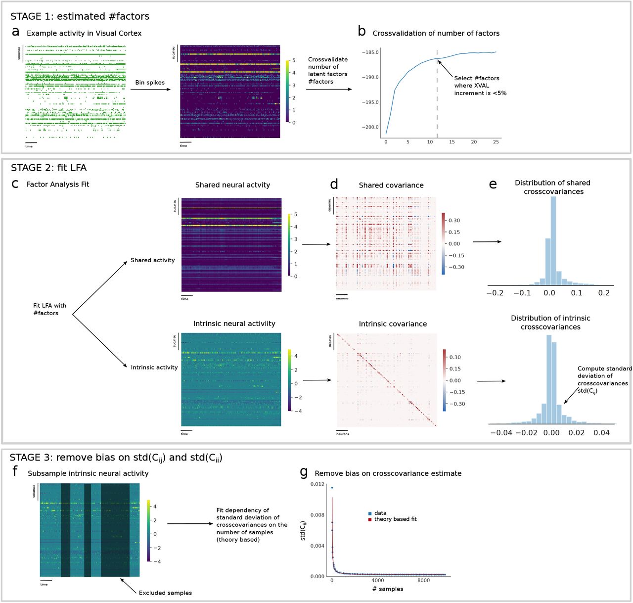
a) For each experimental recording the first step is to bin the spikes to obtain spike count vectors. We use 100ms as a temporal binning window, b) We perform a 5 fold cross-validated latent factor analysis (LFA) with an increasing number of factors (from 1 to 25). For each LFA the log-likelihood is computed and plotted as a function of the number of factors. We select the number of factors (#factors) where for the first time the cross-validation curve has a relative increment which is lower than 5%. c) We perform LFA with the selected number of factors obtaining an estimate of the shared neural activity component and the remaining intrinsic neural activity component. The total activity is given by the sum of the two components. d) We compute the covariance based on the neural activity for both the shared and intrinsic component. e) We compute the distribution of cross-covariances and autocovariances (not-shown) for the two statistics (shared and intrinsic). f) We subsample the intrinsic neural activity obtained at stage 2 c) and based on such subsampled statistics we recompute the standard deviation of cross-covariances (std(ci≠j)) as a function of the number of trials (spike count vectors) used. g) We fit the dependence of std(ci≠j) on the number of trials to estimate and remove the bias induced by the limited statistics.
Second, estimates of cross-covariances are biased due to finite sampling. To remove the bias in the estimation of s (Fig. 1c) due to the limited number of neurons and samples (cf. Sec. S3)) we split neural activities into shared and intrinsic components and then carried out a subsampling procedure to fit the dependence of cross-covariances based on the number of samples. This yielded an unbiased estimate of s, Figs. S3f to S3g. Importantly we also show that using a cross-validated Principal Component Analysis, in place of LFA, yielded similar results (Fig. S5). Applying this procedure to our network model yielded a conservative estimate of the recurrent coupling strength R, as shown in Fig. S6 (cf. Sec. S4).

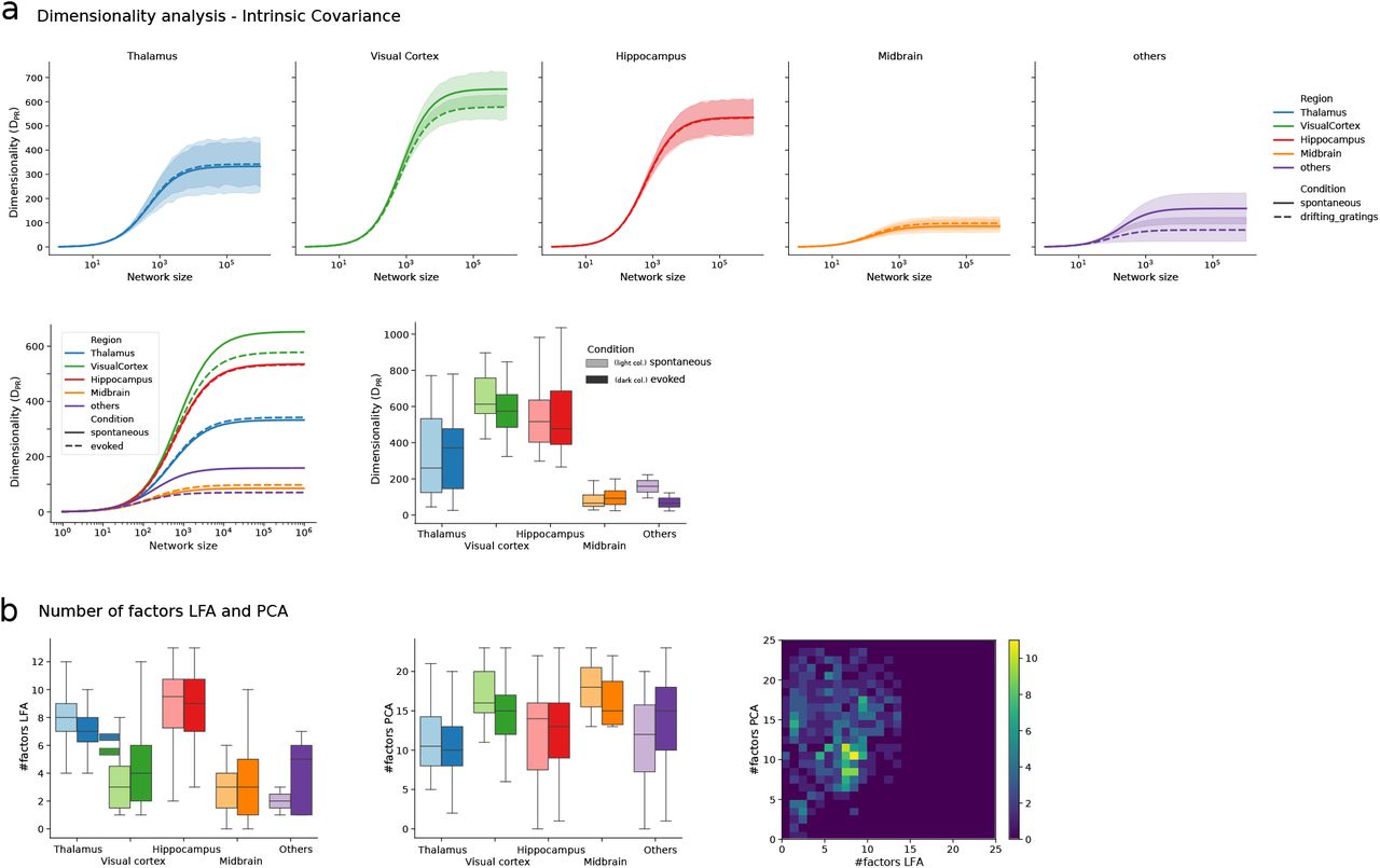
a) Extrapolated dimensionality based on the full covariance for individual brain regions as a function of the network size, cf Sec. S2. Shaded area indicates confidence interval for variability across sessions. b) Same as a) for the intrinsic covariance.

In this figure we represent the plots of Fig. 1 and Fig. 2 obtained by using a cross-validated PCA in place of a cross-validated LFA in the method used to estimate the shared and intrinsic activity components (cf. Fig. S3). a) Top: dimensionality of intrinsic covariance extrapolation across brain regions and conditions. Same as plots shown in Fig. S4. Bottom left: Average of the dimensionality extrapolation in each top panel. Same as Fig. 2d left. Bottom right: dimensionality of intrinsic activity across regions and conditions visualized as a box plot (the box displays average and first top/low interquartile). b) Left: number of factors extracted by the cross-validated LFA technique across regions (cf. Fig. S3). Middle: number of factors extracted by the cross-validated PCA technique across regions. Right: comparison between number of factors extracted by cross-validated LFA and cross-validated PCA. There is a significant correlation (p-value 0.037) between the number of factors extracted with the two methods across experimental sessions.

Correlated external inputs can strongly alter covariances within the network. A rank-one input (panels a,b), for example, can lead to broader distributions (panel a) and altered spectra (panel b) of covariances C (red) with respect to intrinsically generated covariances Cintrinsic (blue). Applying LFA, inferred intrinsic covariances  (green) recover features of ground-truth intrinsic covariances Cintrinsic well over a wide range of spectral radii and ranks of external input covariances, resulting in overall large correlation coefficients
  (panel c), and well matching inferred spectral radii (panel d) and participation ratios (panel e). For large spectral radii R ⪅ 1, LFA wrongly subtracts low-dimensional components of intrinsic covariances, which, however, consistently leads to conservative results, i.e. underestimated spectral radii and overestimated dimensionalities. Note that color scales in panels d and e are cut at the value 2 for better visibility.
A key fact is that Cintrinsic depends on the operating point, identified by the activity profile of the neural population and other neural properties (e.g. adaptation mechanisms, gain modulation etc.). As a result, the recurrent coupling strength is dependent on the underlying experimental condition, as illustrated by the different working points in Fig. 1d. We thus inferred the recurrent coupling strength R for each brain region and experimental condition (spontaneous and evoked activity). To do this we measured s as described above, inserted it in Eq. (1), and plotted the resulting value of R corresponding to different estimates of the overall size N of the underlying recurrent network (Fig. 1e). For values of the network size N ≥ 106 the spectral radius across all regions and both conditions was predicted to be at least R = 0.95 on a scale from 0 to 1, with 1 marking the threshold to linearly unstable activity. As recent experiments report a cell density across the mouse cortex to fall in between 0.48. 105 cells/mm3 in orbital cortex to 1.55. 105 cells/mm3 in visual cortex (63), these results are consistent with neural activity being generated by neural networks operating in a strongly recurrent regime.
Differences in inferred values of the recurrent coupling strength R across conditions correspond to changes in the operating point of the underlying neural networks. To verify the robustness of such estimates we compared, in the evoked condition, values of s obtained by selecting trials based on stimulus orientation for drifting gratings confirming that our results were consistent across orientations (Fig. S7). In the spontaneous condition, known to be strongly influenced by behavioral components (28) but lacking a trial structure, we extracted periods of stationary activity by a cross-validated Hidden Markov Model (HMM) procedure, Fig. S8. The HMM analysis mapped intervals in the spontaneous activity to a number of hidden latent states whose appearance correlated with the change in behavior of the animal (Figs. S8a to S8c). We then compared the values of R obtained separately in stationary periods corresponding to the same latent state, to the value of R obtained in the entire interval of spontaneous activity. The values generally agreed, showing that our analysis is robust to the influence of behavioral components (Figs. S8d to S8e).

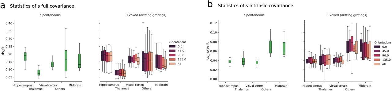
a) Quantity s (defined as the ratio between the standard deviation of cross-covariances and the average of autocovariances) for the full covariance of the activity. Left: spontaneous condition across regions. Right: evoked condition across regions for different stimulus orientation and for all stimulus orientations together. Results in the main figures (Figs. 1 to 2) are computed, for each session, as the average across the four different orientations presented here. b) Same as a) for the intrinsic covariance.
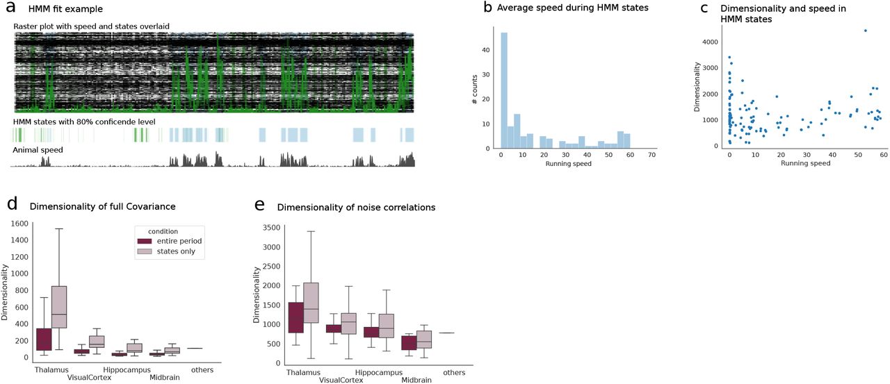
Here we analyse the spontaneous activity by detecting in the interval (30min) of spontaneous activity periods where the neural activity was well captured by different discrete latent states (hypothesis underlying HMM algorithm). The HMM returns a parsing of such periods (30min) into different underlying states by means of an unsupervised detection algorithm. a) Example raster plot during one of the sessions with overlaid running speed of the animal (green). The HMM extracts different states whose appearance strongly correlates with the animal movement. b) Average speed of the animal in a HMM state across all sessions. States appear to correspond to either static or moving conditions for the most part. c) Dimensionality of the neural activity in each state versus the average speed in each state. There exists no significant correlation between the two. d) Dimensionality of the full covariance across regions computed for the entire period of the spontaneous condition or for each individual state (cf. Methods) and averaged across all states and sessions in each brain region. The dimensionality computed over the entire period is systematically higher as the HMM extracts periods where the neural activity tends to be stationary thus limiting the effect of shared variability modes on the dimensionality of the full covariance. e) Dimensionality of intrinsic covariances computed across regions for the entire period or during states only. The dimensionality computed in the two ways appears more in agreement than in panel d) suggesting that the LFA analysis (Fig. S3) successfully extracts components of shared variability coherently in a way comparable to what is achieved by parsing the neural activity with a HMM. These plots confirm the robustness of our estimation method validating the ability of the LFA analysis to capture sources of shared variability in the spontaneous condition.
Sensitive controllability of dimensionality
In the previous section we presented evidence that neural networks across the mouse brain operate in the strongly recurrent regime. We now show that this corresponds to a fundamental statistic of neural activity – its dimensionality – being under sensitive control of the recurrent coupling strength R. To address this question we study the participation ratio DPR, a measure of linear dimensionality which accounts for the extent to which neural responses are spread along different axes directions; in many often-encountered settings DPR corresponds to the number of principal components required to capture roughly 80% of a signal’s variability (27) (Fig. 2a). DPR is given by
 where λi is the eigenvalue associated with the i—th principal component. This measure can be rewritten in terms of the statistics of the covariance matrix (64) (Fig. S2b) and, in large balanced networks of size N, its leading contribution comes from the relative dispersion s of intrinsic cross-covariances across neurons
  (cf. Sec. S1). Combined with Eq. (1), this yields a one-to-one relation between the dimensionality of intrinsic covariances and the spectral radius DPR(Cintrinsic) = N(1 — R2)2, Fig. 2b (for an alternative derivation based on the spectrum of covariance eigenvalues, see (52)). While we formally derived this relation for homogeneous inhibitory networks of rate neuron models (cf. Sec. S1), it robustly generalizes to more complex network topologies as well as nonlinear spiking neuron models (Fig. S9).

The participation ratio can be expressed in terms of three quantities: mean cross-covariances (panel a) as well as standard deviations of auto-(panel b) and cross-covariances (panel c), each rescaled by mean autocovariances. In each panel, solid lines indicate simulations of homogeneous inhibitory networks with leaky integrate-and-fire neuron models and dashed lines show analytical predictions using linear response theory. The matching theoretical predictions for the statistics of covariances yield an accurate prediction for the participation ratio (panel d) for homogeneous single population inhibitory networks (blue) as well as homogeneous two-population excitatory-inhibitory networks (red) and spatially organized single-population inhibitory networks (green).

a) Schematic of activity of a network, where each point represents the activity vector for a specific moment in time and the axis labeled as λ’s represent the covariance principled axis on which the dimensionality (PR) is computed. b) Dimensionality as DPR for a balanced (green) and excitatory (red) network as a function of the spectral radius R. Blue and green curves overlap. c) Absolute value of the relative modulation of dimensionality as a function of the spectral radius, Eq. (4). Blue and green curves overlap. d) Example of extrapolation of dimensionality. Blue is from recordings and red is the theoretical extrapolation. e) Left: Dimensionality extrapolation as a function of network size for the full covariance before applying Latent Factor Analysis (LFA). Lines represent mean values and error bars are shown in Fig. S4. Right: Dimensionality based on full covariance across brain regions for a network of size N = 106 neurons. Boxes capture lower and upper interquartile range of the variability across experimental recording sessions. f) Left: Dimensionality extrapolation based on intrinsic covariances upon applying LFA. Right: Dimensionality based on intrinsic covariances for a network of size N = 106 neurons. g) Example estimation of critical exponent alpha from the normalized spectrum of the full covariance matrix. h) Distribution of critical exponents α across all sessions.
The relationship between DPR and R shows that the dimensionality of the network smoothly decreases with increasing spectral radius towards R =1, which is the coupling level at which the network becomes (linearly) unstable, Fig. 2b. In strongly recurrent regimes like the one just highlighted (R ⪅ 1) the network’s dimensionality is substantially smaller than its number of neurons. Networks close to linear instability have previously been discussed in relation to chaos, and in terms of computational properties as well as topological and dynamical complexity (32, 65–70). The crucial property that we highlight here, and later exploit, is that in strongly recurrent regimes relative change in dimensionality with respect to R (Fig. 2c):
 is greatest. Thus, networks with strong recurrent coupling, R ⪅ 1, achieve a sensitive control of their dimensionality as a function of this coupling strength.
The decreasing relationship between dimensionality and spectral radius R of Eq. (4), together with the high values of R estimated above for regions across the mouse brain (Fig. 1e), suggest that the dimensionality will be low – and hence in a regime where it is under sensitive control – for these brain regions as well. We confirm this next.
To compare recordings where different numbers of neurons were registered, we developed a theoretically unbiased extrapolation of the dimensionality as a function of the number of neurons recorded Nrec (cf. Sec. S2 and Fig. S10). This enabled us to extrapolate the estimates of dimensionality up to realistic values of the size of local circuits  shown in Fig. 1e. By construction, in balanced networks, this extrapolation saturates at DPR = 1/s2 for the dimensionality of intrinsic covariance, while it is a function of multiple moments of the covariance statistics for the dimensionality of the full covariance (cf. Sec. S1-2).

a) Statistics of covariances based on activity from Nrec recorded neurons of a homogeneous inhibitory network of N = 10000 leaky integrate-and-fire neurons. The participation ratio can be expressed in terms of three quantities: mean cross-covariances (red) as well as standard deviations of auto- (blue) and cross-covariances (green), each rescaled by mean autocovariances. The covariance statistics being independent of the number of recorded neurons Nrec allows for an unbiased dimensionality extrapolation based on subsampled covariances. b) Measured dimensionality (black dots) based on statistics of covariances from different numbers Nrec of recorded neurons as well as extrapolated dimensionality (yellow curve) based on covariance statistics of Nrec = 500 neurons (corresponding to yellow dot). The extrapolated dimensionality fits the true dimensionality well. Statistics of covariances are averaged over 100 random subsamplings for each Nrec to avoid statistical fluctuations.
Applying the procedure above to the Allen Institute neuropix-els data showed that the extrapolated dimensionality of the full covariance (cf. Figs. 2d to 2e) saturated for network sizes  , at values on the order of ~ 100 dimensions. On the other hand the dimensionality of intrinsic covariances saturated at higher values of several hundreds of dimensions, Fig. 2f. These two estimates can be taken as a lower and upper bound, respectively, of the dimensionality of the network’s activity, which thus appears to be consistently described by a few hundred dimensions – across all brain regions. This is small number when compared to the number of neurons in the network: indeed, for a network of 105 neurons this corresponds to a dimensionality of less 1% of its size. We note that the number of latent modes individuated by Latent Factor Analysis for the shared covariance was consistently lower 16 across all experimental sessions (Fig. S5d).
Before moving to a more detailed analysis and interpretation of dimensionality within brain areas, we confirm that our techniques reproduce two established effects. The first is that stimuli are known to reduce the dimensionality of responses in cortical activity (64, 71). We found that in the evoked condition, vs. the spontaneous, the dimensionality of activity in visual cortex and hippocampus was indeed significantly lower. The second is a recent estimate of the dimensionality of cortical responses to visual stimuli (26). This measure was based on a power law functional form for the n-th eigenvalue of the covariance matrix that has been shown to emerge in the strongly recurrent regime (52,72): λn = βn-α. Our data appears to converge to such functional form (26, 72), and under the assumption that the eigenvalues have a perfect power-law distribution there exists a one-to-one relationship between the dimensionality of Eq. (3) and the exponent a given by:
 where ζ is the Riemann Zeta function that is obtained in the limit Nrec → ∞. The extrapolation procedure used to determine the dimensionality DPR (Fig. 2f) is in correspondence with the power law fit of the full spectrum of intrinsic covariances (Fig. 2g). Inverting such relation allowed us to compute the distribution of exponents α’s (Fig. 2h) matching the values previously found (26). These results serve to further validate our framework and techniques extending previous experimental findings to other brain areas. They also open the door to a novel way to assess whether neural activity across the brain displays the characteristic features of a physical system operating near criticality (26, 32, 66, 72). We concluded that neural networks in regions across the brain, and across experimental conditions, operate in a regime where where their dimensionality is under sensitive control by the net strength of recurrent coupling R. We can interpret this as the ability to flexibly set the number of modes that might participate in a computation, a feature which may play a substantial functional role across the brain.
Dimensionality across the visual hierarchy and cortical layers
Does dimensionality of neural responses underscore information processing in neural circuits? We reason that in this case the ability of local circuit connectivity to modulate the global dimensionality of neural responses, described above, would acquire a functional role in circuits across the brain.
Several studies in deep and recurrent artificial neural networks have highlighted how dimensionality modulation (compression and expansion) in neural representations across network layers (6, 73) and stages of learning (7, 74, 75) have functional roles in information processing. We next compute dimensionality on a finer scale that for the regions studied above – here for areas that subdivide those regions – to test this idea in data from diverse neural circuits. We focus first on the dimensionality of the full covariance, and then on the intrinsic dimensionality.
Specifically, we first studied the full activity of areas across the visual functional hierarchy (54). Analyzing the full covariance for the neuropixels electrophsiology data revealed a trend of dimensionality expansion from primary visual to higher visual cortical areas, Figs. 3a to 3c and Fig. S11a. Such a trend is consistent with the hypothesis that the visual stream performs a stimulus-dependent dimensionality expansion, akin to the trend described in artificial neural networks and often explained in terms of feature expansion of the input, Figs. S11a to S11b (6,73,76). We note that (77) recently studied the related but distinct quantity of “object manifold dimensionality” computed across transformations of a visual object, in optical recordings from some of these same areas, and found distinct trends for that quantity that are also consistent with dimensionality playing a role in visual information processing. These results underscore the functional value of both dimensionality mechanisms and the visual hierarchy per se (54).

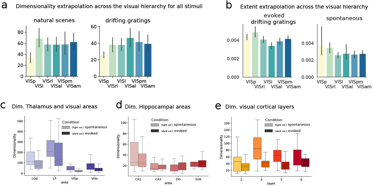
In this figure we provide supplementary plots to the analyses shown in Fig.3. Fig. S11a) Dimensionality of evoked responses for the full covariance across all stimuli in the drifting gratings (i.e. across all orientations as for condition “all” in Fig. S7) and natural scenes (cf. Methods and Fig. S1). Significant increase in dimensionality from primary to higher visual cortical areas. Fig. S11b) Extent analysis across the visual hierarchy. The increase in dimensionality across the visual hierarchy has important connections with the processing of information in artificial deep neural networks classifying images (6, 73). To provide further data for such comparison we analyze the measure of extent of neural representations across the hierarchy  . Such a measure exploits the same statistics of the dimensionality Eq. (3) and can thus extrapolated with identical techniques. Here we plot the average extent across orientations for the evoked drifting gratings condition and the average extent in the spontaneous condition (same as Fig. 3b). The significant decrease in extent for neural representations, together with the increase in dimensionality across all conditions, suggests an increased separability of neural representations along the visual hierarchy. Fig. S11c) Dimensionality of the full covariance across thalamic and visual areas. Secondary visual areas are here considered together (VISs). Fig. S11d) Dimensionality based on the full covariance for hippocampal areas. Fig. S11e) Dimensionality based on the full covariances across visual cortical layers.

a) Dimensionality extrapolation as a function of number of neurons in the network based on the full covariance across areas involved in the visual hierarchy (54). b) Dimensionality analysis from the full covariance, across the visual hierarchy, extrapolated dimensionality for 106 neurons (left and middle panels display the same evoked statistics in the form of a box and bar plot respectively to visualize the full statistics and the significance of the results). Right panel displays the dimensionality for the spontaneous condition showing a non-significant increase. c) Left: Ranked dimensionality analysis of full covariance across areas of the visual hierarchy for the evoked condition. Box color shows fraction of recordings (on a total of number of session times number of stimulus orientation for drifting gratings) where the dimensionality of areas reported in the rows is higher than the dimensionality of areas reported in the columns. Right: quantification of the visual hierarchy for each area. Combined median of functional delay for each pair of cortical areas. Box color reflects the shift from zero in milliseconds in the cross-correlogram between neurons from two areas. Analysis and plot reproduced from (54) with permission of the authors. d) Dimensionality across the visual hierarchy based on the intrinsic covariance. e) Dimensionality of intrinsic covariances for thalamic and visual brain areas. VISs corresponds to the activity of all secondary visual areas. f) Dimensionality of intrinsic covariances for hippocampal brain areas. g) Dimensionality of intrinsic covariances across visual cortical layers. For supplementary plots regarding the dimensionality of full and intrinsic covariances see Fig. S11
The dimensionality of intrinsic covariances was consistent with the hypothesis of visual cortical circuits being strongly recurrent regime, where dimensionality is under sensitive control. While the same trend of increasing dimensionality across the visual cortex hierarchy was not present (Fig. 3d), there were robust trends from thalamic to primary and secondary visual cortical areas (LGd and LP to VisP and VISs, Fig. 3e) and across hippocampal areas (CA1, CA3, DG, SUB), Fig. 3f, suggesting robust differences in their intrinsic connectivity. Overall, areas considered to be possible input regions to broader circuits (LGd, LP and CA1) displayed a high dimensionality corresponding to a less recurrent, and potentially more feed forward, circuit, when compared with their visual cortex and hippocampal counterparts. The area CA3 in particular, known to have strong recurrent connections (78), appeared to have the lowest dimensionality of intrinsic covariances in line with such assumption.
Finally we considered whether different cortical layers could carry out similar functional roles in expanding or reducing the dimensionality of neural representations. We found that layers 2 and 5 had respectively the lowest and highest dimensionality. Intriguingly, this result is consistent with the hypothesis that layer 2 performs computation through strongly recurrent circuitry (29), Fig. 3g.
These systematic trends across brain areas and layers, in both the full and intrinsic dimensionality, suggest that the modulation of dimensionality across brain networks can be associated with functional information processing. The robust trends we described for intrinsic dimensionality reveal the potential for local circuitry to tune this dimensionality, a topic to which we turn in more detail next.
Local synaptic motifs enable tuning of recurrent couplings
We next asked how, on the level of circuit connectivity, neural networks can regulate their local recurrent coupling strength R and hence their dimensionality. We reasoned that the recurrent coupling strength is ultimately derived from properties of anatomical connectivity. We thus hypothesized that, as for excitatory regimes in (5), local synaptic motifs would regulate the dimensionality of the network’s activity.
It is well known that globally increasing or decreasing synaptic strengths in a neural network affects its spectral radius (68). However, assessing overall network synaptic strengths based on synaptic physiology datasets is challenging, and strengths alone are not the only important aspect of connectivity. Here we develop theoretical results to show how local synaptic motifs, that can be more easily identified in synaptic physiology datasets, significantly modulate the spectral radius over and above overall synaptic strengths. The special case of networks with only reciprocal connections is well studied (13, 79). Here we develop a general theory for homogeneous networks that takes full account of any second order motif; these are statistics of the neural connectivity W that involve dependencies between any pair of connections (see Methods). A complimentary theoretical approach via the spectrum of the covariance matrix (52) yields results consistent with the theory developed here. Second order motifs appear in four types: reciprocal, divergent, convergent, and chain motifs, together with the variance of neural connections already present in purely random models (80). These have been shown to cover important functional roles in circuit computations (5, 12, 14, 48) and emerge from learning rules consistent with biological STDP mechanisms (81, 82). Our theoretical analysis yielded a novel compact analytical quantity:
 where τrec, τch, τdiv, τcon denote correlation coefficients between pairs of synapses that capture the abundance of reciprocal, chain, divergent, and convergent motifs, respectively (cf. Methods and Sec. S5-6). Here σ captures the variance of network’s connections, which, similar to the motif statistics τ, is assumed to be the same for all connections. This formula describes how the spectral radius R is affected by increasing or decreasing the statistics of second order motifs (Fig. 4a) and thus links the modulation of auto- and cross-covariances and the dimensionality of neural responses to the prevalence of local circuit motifs, shown in Figs. 4a to 4b. This link between local anatomical features of the connectivity and the global network property R opened the way for probing the functional role of local circuit motifs, in synaptic physiology datasets, in regulating the network’s recurrent coupling.

a Theoretical dependence of spectral radius on motifs abundance, for individual motifs. b Theoretical dependence of dimensionality on motif abundances for individual motifs. c Motif abundances, measured by means of connection and motifs probability of occurrence, in mouse V1 based on all synapses (both excitatory and inhibitory). Inset: Motif abundances computed separately for just excitatory or inhibitory synapses. d Same as c) for the human synaptic physiology dataset. e Estimation of Rmotifs from data for 100 bootstraps, each based on a random subset of 50% of experimental sessions. Shuffle of the synapses within each experimental session and across all experimental sessions is shown, also based on 100 bootstraps of 50% of the experimental sessions. f Same as e for the human dataset.
Cortical circuits employ local synaptic motifs to modulate their recurrent coupling
We analyzed synaptic physiology datasets (55) to assess the involvement of synaptic motifs in modulating the recurrent coupling strength. The spectral radius defined by Eq. (6) has an overall scaling term, σ, and a motif contribution term given by Rmotifs = R/σ which encapsulates whether the overall motif structure is contributing to increase (Rmotifs > 1) or decrease (Rmotifs < 1) the spectral radius R. While the absolute value of synaptic strengths, and thus R, cannot be robustly linked to the theory from neurophysiology datasets, it is possible to assess the probability of occurrence of individual motifs estimating Rmotifs, cf. Methods. Our theoretical results and data analysis thus far led us to hypothesize that if local circuit motifs modulate spectral properties of the neural circuit, then their value must be sensitively different from zero. In line with our findings, values of Rmotifs > 1 would point towards motifs being tuned to reduce the dimensionality while Rmotifs < 1 would indicate an opposite contribution; but either scenario would confirm the involvement of motifs in regulating our estimates of recurrent coupling strength and hence dimensionality.
We sought to verify these hypotheses in two ways: by reviewing existing studies of circuit connectivity, and by new analyses of recently released, very large-scale, neurophysiology data where all the synapses among 4 to 8 cells were simultaneously probed in-vitro. These new experiments were carried out on both mouse and human cortex (55), and draw up on the large-scale publicly available Synaptic Physiology Dataset from the Allen Institute for Brain Science (cf. Methods).
Existing literature on circuit motifs reports a consistent increased prevalence of reciprocal connections across species and brain areas (16, 83–85); indeed, to the best of our knowledge only one study has not found a significant overexpression of reciprocal motifs when compared to random statistics (86). As reciprocal connections are the only ones whose increased occurrence elevates Rmotifs, these results are consistent with Rmotifs > 1. Only one of these studies computed the statistics of all motifs up to third order (16) and, reanalyzing their results, we found that the motif statistics they reported pointed to Rmotifs = 1.38, in line with our prediction.
We then turned to analyze a synaptic physiology dataset (55), consisting of 1368 identified synapses from mouse primary visual cortex (out of more than 22000 potential connections that were tested) and 363 synapses from human cortex. We first computed the statistics of individual motifs across both datasets for all connections, shown in Figs. 4c to 4d, and then restricted the computation to only excitatory and inhibitory synapses for the mouse dataset where the statistics of the available data allowed us to do so (Fig. 4c inset). We inferred the motif contributions to the spectral radius for the mouse dataset across all layers  , for the human dataset
  and also for the excitatory only connections in the mouse
  , confirming a substantial role for motifs in regulating the recurrent coupling strength of the networks, Figs. 4e to 4f.
While the statistics of the data did not allow the estimation of Rmotifs in individual layers of the visual cortex due to the low number of synapses measured within each layer (and more specifically in layer 5), our theoretical analysis coupled with our findings from the electrophysiology (Fig. 3e) led to a clear experimental prediction: that the local effective recurrent coupling strength R would be stronger in layer 2 than in layer 4 or 5. This prediction awaits confirmation in larger synaptic physiology or circuit reconstruction datasets (87).
Conclusion
We showed that neural networks across the mouse brain operate in a strongly recurrent regime. A feature of this regime that may have an important impact on computation is that neural circuits can sensitively modulate the dimensionality of their activity patterns by modulating their recurrent coupling strength. Indeed, novel analyses of massively parallel neuropixel recordings from areas within the thalamus and hippocampus display clear trends in the dimensionality of intrinsic covariances. Our theory links these findings to clear predictions for recurrent coupling strength in these areas: a higher dimensionality suggests a lower recurrent coupling strength and vice-versa. Our findings agree with current knowledge of the function of these areas, in which LGd, LP, CA1 serve as input areas to cortical and hippocampal areas with greater recurrent coupling. A similar trend arises by comparing the activity dimension in layer 2 vs. deeper layers in cortex.
We showed that the critical circuit features that determine a circuit’s recurrent coupling strength R – and hence the dimensionality of its activity patterns – are not just its overall synaptic strength, but also a tractable set of local synaptic motifs that quantify how these synapses are arranged. This follows from new theory based on beyond mean-field calculations. Experimental evidence for the role of motifs in regulating activity dimension arises from our analysis of synaptic physiology data. This shows that a measurable quantity Rmotifs, quantifying the contribution of motifs to recurrent coupling over and above that of synaptic strength, is significantly increased in cortical circuits in both mouse and human (Figs. 4e to 4f).
In sum, we provide new evidence that circuits across the brain operate in a strongly coupled regime, and reveal a set of mechanisms that they have at their disposal for regulating what may be the most fundamental feature of their collective activity: its dimensionality. Our theoretical advances enable a new connection between large-scale electrophysiology and synaptic physiology datasets, and provide a new measurable quantity Rmotifs as a target for upcoming connectivity datasets. This work advances new theory and brain-wide experimental analysis that add to recent evidence for an attractive and simplifying idea: that connectivity exerts control over the network responses in a highly tractable manner, by determining its global properties in terms of the statistics of its local circuitry.
Supplementary notes
As we were finalizing the writeup and experimental figures in this manuscript, independent theoretical work (52) was reported, as cited above. This independent work uses a powerful but different approach – based on computing the spectral density – to achieve complementary theoretical results related to the ones we describe here. While full details of the calculations underlying the results of (52) have to our knowledge not yet appeared, we are confident that the future will see interesting and productive further analyses of the relationship between the work in (52) and the present theoretical framework.
Methods
Electrophysiology dataset
Data were obtained from the public repository of the Allen Institute for Brain Science (53, 54) where all details regarding mice, surgeries, intrinsic signal imaging, habituation, behavior training, implants, recordings and spike sorting can be obtained – as well as publicfacing visualization and open software tools. We summarize some of this information here. These recordings contain 57 experimental sessions in adult mice. Each mouse was implanted with a 204 stainless steel headframe with a cranial window that was glued to a black acrylic photopolymer. Mice underwent two weeks of habituation in sound-attenuated training boxes containing a running wheel, a headframe holder, and stimulus monitor. At the beginning of the experimental session the cranial coverslip was replaced with an insertion 920 window containing holes aligned to six cortical visual areas. Mice were lightly anesthetized with 921 with isoflurane. Neural recordings were performed with 6 Neuropixels probes each containing 960 recording sites providing a maximum of 3.84 mm of tissue coverage. Visual stimuli were generated using scripts based on PsychoPy and followed one of two stimulus sequences (“brain observatory 1.1” and “functional connectivity”), Table S1 and Fig. S1. Of these we analyzed only those corresponding to “functional connectivity” as they included a period of spontaneous activity which “brain observatory 1.1” didn’t include.
Electrophysiology data preprocessing
To perform the analysis we used and extended the Allen SDK toolbox https://github.com/AllenInstitute/AllenSDK. We extracted periods in the stimulus presentation sequence corresponding to the two conditions analyzed: spontaneous and evoked activity. The latter corresponded to “drifting gratings 75 repeats”. Each repeat, in one of 4 orientations and 2Hz temporal frequency, lasted 2sec with intertrial intervals of 0.5sec. Spontaneous activity was recorded for 30min while the animal was in front of a screen of mean grey luminance. While for the spontaneous conditions we directly binned the entire period of 30min into 100ms windows as a starting point of our analysis (Fig. S3), for the evoked condition we considered, for each stimulus presentation, the window 0.4-2.0sec after stimulus onset binning spikes in this window into 100ms non-overlapping bins. Such a window was identified to avoid transients in the neural activity evoked by the stimulus presentation. We then performed the intrinsic covariance analysis on 5 different sets of spike counts: one corresponding to spontaneous activity and 4 corresponding to the 4 orientations of drifting gratings, each having 75 trials with 16 bins of 100ms. Across all analysis we used only recordings, for a specific brain region or brain area, where at least 20 neurons were simultaneously recorded.
Dimensionality analysis
We analyzed the measure of dimensionality DPR given by Eq. (3). This measure can be rewritten in terms of four moments of the entries of the covariance matrix (Fig. S2) and the number of neurons recorded Nrec or, equivalently in terms of the network size N (cf. Suppl.Mat.):
 which is formally identical to Eq. (3) but with the network size N being replaced by the number of recorded neurons Nrec. The dimensionality DPR of the recorded activity therefore depends on the number of recorded neurons. In the absence of any bias in the subsampling procedure the statistics of covariances, as extracted by means of our analysis, are invariant (cf. Sec. S3) and Eq. (7) is adopted to extrapolate the dimensionality as a function of the neurons recorded, Figs. 2d to 2f and Figs. 3a to 3c.
Bias correction in the statistics of covariances
We performed a theoretical analysis of the bias, induced by subsampling both neurons or trials, on the covariance statistics (see Fig. S2 (cf. Suppl.Mat.)). Our analysis yielded that the average of auto- and cross-covariances (μ(cii) and μ(ci⪅j) are unbiased while the variances of both auto- and crosscovariances have a bias which decays with the number of trials T as  :
:

For readability we adopted the notation  and
and  and δa = σ(cii) and δc = σ(ci⪅j), where
  indicates the empirical estimate and the non-hat quantities indicate the true values. Based on such analysis we performed a bias correction.
Intrinsic covariance analysis
Under a linear assumption the covariance matrix of neural activity splits into two contributions Eq. (2): a shared and an intrinsic component (cf. Sec. S4). In order to estimate these two components we developed a three stage procedure that could be performed by utilizing different algorithms at its core, here we use Latent Factor Analysis (LFA) and Principal Component Analysis (PCA). In the following we will explain this procedure with LFA but it would equally work with PCA or other algorithms. The first stage bins the spikes of neurons into spike counts within non-overlapping windows. We used 100ms bins, Fig. S3a. Then we performed LFA with an increased number of hidden factors and computed the log-likelihood as a function of factors with a 5-fold cross-validation technique, Fig. S3b. We selected the number of factors by choosing the corresponding point in the log-likelihood curve where the cross-validated log-likelihood didn’t increase more than 5% for the first time. This functioned as a robust estimation of where the plateau or peak in the curve is found, Fig. S3b. The second stage estimated the activity of the shared neural activity and intrinsic neural activity by running LFA with the selected number of components, Fig. S3c. The computed shared and intrinsic covariance (Fig. S3d) yielded a first estimate of the standard deviation of intrinsic cross-covariances σ(ci⪅j), Fig. S3e. In the third stage 3 we removed the bias on such estimates by subsampling the intrinsic neural activity (Fig. S3f) and computing σ(ci⪅j) as a function of the number of used samples T (Fig. S3g). We then fit a dependence  to extract the true value of σ(ci⪅j) from the estimates
  . All analyses were run through custom scripts based on the scikit learn library.
Hidden Markov Model analysis
The Hidden Markov Model (HMM) analysis of spontaneous activity followed a two stage procedure and was performed by means of the ssm toolbox (https://github.com/lindermanlab/ssm). In the first stage we used the spike counts obtained in Fig. S3a and ran a 5-fold cross-validated estimate of the number of hidden states. For an increasing number of hidden states (1 to 15) we fitted a cross-validated HMM and computed the log-likelihood of the fit. We then selected the number of states with an elbow detecting algorithm using the kneed toolbox (https://github.com/arvkevi/kneed) with parameter S = 1. We then fitted an HMM with the so found number of states to the spike counts. The output of the HMM analysis was a confidence (0-100%) for the neural activity in each bin to be generated by each of the underlying hidden factors. We thresholded this confidence (to 80%) so as to select only temporal intervals where the algorithm isolated a specific hidden factor as responsible for the collected neural activity, Fig. S8a. Overall we found that most factors would coincide with the animal being either moving or still Fig. S8b. Once all time points, and in turn spike-count population vectors, were tagged with one or no hidden states we used all such vectors tagged with the same state to compute a state specific covariance capturing neural variability for each individual state. We then averaged across all states in each session to generate the estimates used in Figs. S8d to S8e.
Synaptic physiology dataset and analysis
We analyzed publicly available data collected at the Allen Institute for Brain Science ((55), Synaptic Physiology Dataset https://portal.brain-map.org/explore/connectivity/synaptic-physiology). The data consisted of over 22000 probed synaptic connections resulting in 1368 chemical synapses from mouse primary visual cortex and 363 from human cortex, obtained via simultaneous patch clamp recordings.
Our theoretical analysis developed a measure of recurrent coupling strength which was derived in the context of homogeneous networks where the motif statistics of excitatory and inhibitory populations were assumed to be the same. Because of this theoretical assumption we analyzed the data both exploiting and omitting information regarding the nature (excitatory or inhibitory) of individual synapses. For each synapse the data reported the source and target neuron type (excitatory and inhibitory) and a number of other variables. To estimate Rmotifs in each dataset or subset of data (bootstraps) we proceeded as follows: We first computed the probability p of having a synapse among two neurons and estimated the variance to be σ = p(1 — p) according to Bernoulli statistics. We then computed the probabilities of having a reciprocal, chain, convergent or divergent motif in the data by computing the total amount of motifs in each category and dividing by the total amount of neuron’s pairs (or triplets) which could carry such motif. This returned the raw probabilities for each motif which, after subtracting p2, we divided by σ to obtain τrec,τchain,τdiv,τcon. Finally, we applied the formula in Eq. (6) to obtain the spectral radius. A more detailed description can be found in Suppl.Mat. Error bars in Figs. 4c to 4d were obtained as 95% confidence interval of the estimated mean of motif counts according to standard error propagation techniques in count distributions (see python statsmodel library proportion and proportion_confint). Importantly the analysis just described didn’t include information regarding whether the synapses were excitatory or inhibitory if not for the inset in Fig. 4c, where we show that the statistics of inhibitory and excitatory motifs are not significantly different. For Figs. 4e to 4f we similarly analyzed all synapses performing a bootstrap analysis. For each bootstrap we subsampled the entire statistics 100 times into 50% random sampling of all experimental sessions. For each bootstrap we either directly computed the radius Rmotifs as just described or shuffled the synapses within each experimental session (shuffle within sessions in Figs. 4e to 4f) or across all experimental sessions (shuffle across sessions in Figs. 4e to 4f).
Network models and linear response theory
We made use of the fact that correlations in spontaneous, asynchronous irregular activity states of spiking networks can be well under-stood using linear response theory (34, 88): starting from a network of leaky integrate-and-fire (LIF) neurons (Fig. S9), linearization around some stationary state maps the statistics of fluctuations to an equivalent set of Ornstein-Uhlenbeck processes coupled via some effective connectivity matrix (89). Ornstein-Uhlenbeck processes are linear stochastic differential equations that can be analyzed using statistical field theory (32, 90). Fig. S9 shows that such theory faithfully predicts the statistics of covariances and dimensionality as a function of the spectral radius of the effective connectivity in direct simulations of LIF neurons. For simplicity, our theoretical derivations thereby focused on homogeneous single-population networks, where recurrent inhibitory feed-back balances external excitatory input to arrive at a balanced state (35). Our dimensionality results, however, generalize well to more complex network topologies Fig. S9d.
Theory of spectral radius in balanced networks with second order motifs
Using the path-integral representation of coupled Ornstein-Uhlenbeck processes (90), we performed an average of the moment-generating function for the network dynamics over the statistics of connections. Second-order connection motifs were thereby incorporated via the covariance tensor Δijkl = 〈WikWjl〉 — 〈Wik〉〈Wjl) between connections Wik from neuron k to neuron i and Wjl from neu-ron l to neuron j. Similar to the case of reciprocal connections (46, 79), the second-order connectivity statistics yield non-Gaussian integrals that cannot be solved exactly. We obtained good approximations to these integrals for large networks by using a saddle-point approximation of auxiliary fields that were introduced for the terms related to the various motif contributions. The associated self-consistency equations for the saddle points showed parameter-dependent divergence structures that we related to connectivity eigenvalues crossing the line of instability of the linear network. By distinguishing between outlier and bulk eigenvalues, this analysis allowed us to infer a theoretical prediction of the spectral radius of the effective connectivity in relation to the various motif abundances, cf. Sec. S5-6.
Numerical validation of motifs theory
Given the possible ranges for different motif abundances in homogeneous single-population networks (cf. Suppl. Mat.), we validated our theoretical predictions for the spectral radius and dimensionality (Fig. 4a,b) using network creation algorithms shown in Suppl. Mat. The spectral radius is well predicted for all values of τ. The same holds true for the prediction of the dimensionality, except for reciprocal motifs, where the prediction is only correct on a qualitative level. The prediction of the dimensionality relies - in addition to our results on the motif dependence of the spectral radius - on the mapping between the spectral radius and the width the covariance distribution that has been derived in (32) for homogeneous random networks using beyond-mean-field techniques. This relation is robust as long as eigenvalue spectra of connectivities show a circular organization in the complex plane (cf. Suppl. Mat.). Convergent, divergent and chain motifs do not strongly alter the shape of the bulk of connectivity eigenvalues (43). Therefore, the theory for homogeneous random networks yields correct quantitative results for these cases. Reciprocal motifs, however, deform the bulk eigenvalues from the circular to an elliptic shape, which causes the minor quantitative mismatch between theory and simulations.
Acknowledgments
We thank Stefan Mihalas, Nicholas Steinmetz, Leenoy Meshulam for helpful feedback on our findings. S.R. was supported by a Swartz Fellowship in Theoretical Neuroscience at the University of Washington, and by NIH BRAIN Grant R01EB026908, and E.S.B. by NIH R01EB026908 and NSFDMS Grant 1514743. D.D. and M.H. were supported by the HGF young investigator’s group VH-NG-1028, the European Union’s Horizon2020 research and innovation program under Grant agreements No. 785907 (Human Brain Project SGA2) and No.945539 (Human Brain Project SGA3), and funded under the Excellence Strategy of the Federal Government and the Länder (G:(DE-82)EXS-PF-JARA-SDS005). We thank the Allen Institute for Brain Science founder, Paul G. Allen, for his vision, encouragement, and support.
Bibliography
- 1.↵
- 2.
- 3.
- 4.↵
- 5.↵
- 6.↵
- 7.↵
- 8.↵
- 9.↵
- 10.↵
- 11.↵
- 12.↵
- 13.↵
- 14.↵
- 15.↵
- 16.↵
- 17.
- 18.↵
- 19.↵
- 20.↵
- 21.↵
- 22.↵
- 23.
- 24.↵
- 25.↵
- 26.↵
- 27.↵
- 28.↵
- 29.↵
- 30.↵
- 31.↵
- 32.↵
- 33.↵
- 34.↵
- 35.↵
- 36.
- 37.↵
- 38.↵
- 39.
- 40.
- 41.
- 42.↵
- 43.↵
- 44.
- 45.
- 46.↵
- 47.
- 48.↵
- 49.↵
- 50.↵
- 51.↵
- 52.↵
- 53.↵
- 54.↵
- 55.↵
- 57.↵
- 58.↵
- 59.↵
- 60.↵
- 61.↵
- 62.↵
- 63.↵
- 64.↵
- 65.↵
- 66.↵
- 67.
- 68.↵
- 69.
- 70.↵
- 71.↵
- 72.↵
- 73.↵
- 74.↵
- 75.↵
- 76.↵
- 77.↵
- 78.↵
- 79.↵
- 80.↵
- 81.↵
- 82.↵
- 83.↵
- 84.
- 85.↵
- 86.↵
- 87.↵
- 88.↵
- 89.↵
- 90.↵


