Large-scale models based on population structure for the spatiotemporal distribution of U.S. porcine epidemic diarrhoea outbreaks

ABSTRACT

In 2013, U.S. swine producers were confronted with the disruptive emergence of porcine epidemic diarrhoea (PED). Movement of animals among farms is hypothesised to have played a role in the spread of PED among farms. Via this or other mechanisms, the rate of spread may also depend on the geographic density of farms and climate. To evaluate such effects on a large scale, we analyse state-level counts of outbreaks and state-level changes in the number of pigs weaned along with variables describing the distribution of farm sizes and types, aggregate flows of animals among farms, and an index of climate. Flows are found to be correlated with cross correlations in outbreak time series. We illustrate when such a relationship might be expected with simulation of a simple model of farm-to-farm spread. We then use stability selection to determine that balance-sheet variables and the number of farms in a state are relevant predictors of PED burdens. We fit a transmission model that estimates effects of both farm density and flows on transmission rates. These results may help connect the modeling of emerging livestock diseases with field data.

Introduction

The 2013 emergence of porcine epidemic diarrhoea (PED)¹ in the United States has provided an example of both the economic hardships livestock diseases can cause and our limited understanding of how such diseases spread. Porcine epidemic diarrhoea virus (PEDV), the causative agent, acutely infects the intestine and causes severe diarrhoea and vomiting.² Currently, the earliest known U.S. outbreak occurred in April,³ and in less than a year PED outbreaks were confirmed in 27 states,⁴ states that together produce 95 percent of the U.S. pig crop.⁵ Farms experiencing outbreaks have suffered 90 percent and higher losses of unweaned pigs.³ The time it takes for a farm to return to stable production is highly variable but on the order of weeks, leading to great expenses in infection control costs and production losses alike.

Losses were also apparent on a national economic scale. Producers had for the previous 8 years been making steady increases in the average litter size of about 0.16 head per year.⁶ By November 2013, the average litter size had begun an abnormal downturn,⁶ dropping 0.66 head by March 2014.⁷ The virus also affected swine production in Asia and other parts of America.^{8, 9}

The mechanisms by which PEDV spread among farms are not yet clear. Transportation-associated transmission of PEDV has been supported by the observation at harvest facilities that it spreads among trailers used to transport swine,¹⁰ and some experts believe that current resources of livestock trailers, trailer-washing facilities, and transport personnel are insufficient to allow for a standard 3-hour trailer cleaning between every load.¹¹ With such concerns in mind, some states responded to PED by requiring that imported swine be from PEDV-free premises. Transportation-independent mechanisms such as airborne particles¹² and contaminated feed^13–16 have also been implicated. Detailed investigations of outbreaks on farms can be inconclusive regarding the mechanism of PEDV introduction.³

Much of the research on PED involves detailed investigations on a small scale. For example, there have been epidemiological investigations of infected farms in North Carolina and a cluster of infected farms in Oklahoma and adjacent states.¹⁷ Such work is effective for determining the biological plausibility of different routes, but the risk-factors identified in a small-scale study may be specific to the small area of the study. Modelling studies based on large-scale surveillance data^18–20 can thus be a valuable complement to such work by quantifying the overall importance of a transmission route across a large population. Such quantification for PED could also be considered a contribution to the general study infectious diseases of livestock. Although animal movements in general are considered a risk for transmission,²¹ only a limited number of studies^{18–20, 22, 23} have quantitatively compared this risk to other competing risks.

Here we present a national-level analysis of the effects of transportation flows, spatial spread, farm density, and climate. We first conduct simple correlations tests for the association between flows, distance, and the similarity of time series of the number of farms experiencing outbreaks. Then we present simulation results to illustrate how one of the observed correlations may arise from a simple model of farm-to-farm spread. We go on to consider a larger group of explanatory variables and apply stability selection to identify those with the most robust association with PED burdens. On the basis of the selected variables, we formulate a simple model of farm-to-farm spread and obtain parameter estimates.

Results

A few preliminary facts pertain to all our results. First, all of the contiguous 48 states share some portion of the nation’s swine but the Midwest and North Carolina are areas of major concentration (Fig. 1a), holding some 88 percent of the inventory.⁵

Second, PED data are available at the state level in the form of weekly counts of the number of diagnostic case submissions that tested positive for PEDV. These counts, reported as positive accessions and shown in Fig. 1b, are likely to be informative of the number of infective farms because each infected farm will submit a limited number of samples for testing. We work with the assumption that positive accessions are correlated with the number of PEDV-positive farms because data on the number of PEDV-positive farms did not become available until June 2014. These more recent data do support our assumption that positive accessions and positive farms were correlated in 2013: positive accessions and positive farms have a Spearman rank correlation of 0.74 with data from June 2014 to February 2015.²⁴ Although it might seem preferable to analyse the 2014 data on positive farms instead of positive accessions, the 2013 data may be more informative of transmission routes because farms protected by immunity rather than lack of exposure were most likely less frequent in 2013.

Third, as a proxy variable for all pathways of spread involving shipment of live swine, we use estimates of swine transport flows. We define these flows as the total number of swine moved between pairs of states each year for purposes other than slaughter. These flows vary greatly in size but generally the larger ones move swine into the Midwest (Fig. 1c). A detailed description of the data we have analysed appears in Supplementary Note 2.

Figure 1.

Spatial structure in the PED epizootic reflects that of swine production. (a) State-level swine inventory estimates in thousands of head. (b) Cumulative positive accessions in each state for 2013, our proxy for the number of farms experiencing outbreaks. (c) Network of estimated annual interstate flows of head of swine. The arrow in the key indicates the direction of flow along the color gradient. (d) Network of cross correlation in weekly positive accessions between states reporting positive accessions in 2013. In both (c) and (d), edges with similar origins and destinations are bundled together to summarise regional patterns.

Correlation tests of pairwise relationships

As a first step in evaluating the relationship between transport flows, space, and the spread of PED, we analysed pairwise correlations. To quantify the extent to which the infections in one state were associated with those in another, we computed the cross correlation with a lag of 1 week between all pairs of states reporting cases (Fig. 1d). The cross correlation is the correlation between the values of one time series and corresponding values in another time series shifted by some lag. Often coupling of population dynamics is measured by cross correlations with a lag of zero, which is indicative of the extent to which time series are synchronized. Here we used a lag of 1 week because we were interested in whether one time series was predictive of another, which would be suggestive of causality. As we discuss in Supplementary Note 4, it is reasonable that farms experience an outbreak within a week of being exposed.

We conducted one-tailed Mantel tests with a significance threshold of α = 0.05 to determine if there were significant positive correlations between corresponding elements of matrices of cross correlations, negative geographic distances, state with shared borders, and flows. The Mantel test evaluates the significance of such an association via a permutation procedure that accounts for the intrinsic dependence among elements of distance matrices.²⁵ Descriptive statistics for the analysed data appear in Supplementary Note 1.

We found that cross correlations were positively correlated with the logarithm of transport flows. This relation held whether flows and cross correlations were treated as directional (Fig. 2a), were averaged over both directions (Supplementary Fig. S1), or were ranked (Supplementary Figs. S2 and S3). The p values for these correlations were all below 0.05 / 6, which means that they would remain significant after using a Bonferroni method of limiting the probability that any false positives occurred in our tests to 0.05. On the other hand, in no case would the correlations between geographic distance and cross correlations remain significant after such a correction. The correlations between an indicator variable of whether a pair of states shared borders and cross correlations were similar to or weaker than those of distance, were not significant after Bonferroni correction, and were not included in the plots to keep them simpler.

The correlation between flows and cross correlations seemed to be driven in part by concentration of both high cross correlations (Fig. 1d) and large flows (Fig. 1c) in Midwestern states. The cross correlations of these states results from the presence of a small wave of positive accessions early in the outbreak and a much larger wave toward the end of our observations (Fig. 2b, left column). Also, Kansas and Oklahoma share a distinctive period of high positive accessions in the middle of the time series and fairly large flows (Supplementary Fig. S4 and Fig. 2b).

Figure 2.

Similarity between state’s PED dynamics correlated more strongly with transport flows than with distance. (a) Scatter plots and Pearson correlations between transport flows, cross correlations between time series of positive accessions, and negative geographic distances. The p values are from a Mantel test. (b) PED dynamics for selected states. Distinct shapes are apparent in the time series of the Midwestern states (MN, IL, IA), Kansas and Oklahoma, and North Carolina.

The flows were themselves correlated with the geographic distance between states, and these distances were in turn correlated with cross correlations (Fig. 2a). Thus we also examined the partial correlation of flows and cross correlations, controlling for geographic distance. This partial correlation was around 0.31 whether directed or undirected relationships were used, and thus controlling for distance does not greatly diminish the correlation.

Having considered the significance of the correlation, we now consider its size. A Pearson correlation of 0.36 (Fig. 2a) indicates that there is not a strong linear relationship between the logarithm of flows and cross correlations. For example, North Carolina’s time series did not correlate strongly with many other states in spite of North Carolina being a major source of swine for many other states (Supplementary Fig. S4). We next use modeling to provide us with a possible explanation for these observations and, more generally, what observations we might expect.

Simulation study of cross correlations

It may at first seem obvious that if transport of animals is associated with transmission, then cross correlations in the number of infected farms between states should increase as transport flows increase. However, the relationship may be more complicated when one considers that the flow may be partitioned among pairs of farms in different ways between different pairs of states. Thus, to aid interpretation of the above correlation, we conducted simulations to clarify how farm-level variation within states could affect the apparent relationship between state-level flows and cross correlations.

Our model tracked the infection status of individual farms and included the full set of relationships by which farms could infect each other. Farms were represented as nodes in a network, and the set of transmission routes as undirected edges. A pair of states was represented by partitioning the nodes into two disjoint sets.

To obtain a simple model of the dynamics of PED, we use a stochastic susceptible–infected–susceptible (SIS) model in which the states of the vertices are either susceptible to infection from any of its neighbours (i.e., other vertices that share an edge with it) or infective and able to spread infection to any of its neighbours. (Full model specifications appear in Methods.) The use of an SIS model is a simplification that does not include the immune state farms are likely to experience following an outbreak, in which no clinical signs are visible and farms may be less infectious. However, the eventual return to a susceptible state in our model is supported by reports²⁶ of farms experiencing two PED outbreaks within about one year of each other. Such reinfections are to be expected because, unless controlled oral exposure or vaccines are regularly used, a farm’s immunity will wane as animals that were exposed to the virus are replaced.

If we consider sets of vertices in each of two partitions, any edges that link vertices in each of the partitions are members of what is called the edge cut set of those partitions—removing those edges would cut off all paths between them. We refer to this set of edges as the cut set for brevity. Our study consists in calculating the cross correlation (with a lag of 1 time step) of the number of infected farms in two states with varying cut sets. The goal is to see how the cross correlation in infected farms between a pair of states depends on both data we have (the flows of swine) and data we do not have (how the flow is distributed among pairs of farms). Clearly, the total flow, size of the cut set, and the number of vertices incident to edges in the cut set are all important variables. We use three schemes to tune these variables systematically to provide insight into how they work together to determine the cross correlation between a pair of states. These schemes, fully described in Methods, cover extreme scenarios in the distribution of cut-set edges among nodes and thus allow for a wide range of possible outcomes. In brief, there is a balanced scheme in which cut-set edges are distributed evenly among all farms in both states, an unbalanced scheme in which one state has hubs which connect to all farms in the other state, and a reciprocally-unbalanced scheme in which both states have such hubs.

As seen in models that assume homogeneous mixing,²⁷ the largest cross correlations typically occur when the population of infected nodes is near critical levels necessary for subsistence and transient flare-ups in the number of infected nodes occasionally occur in one population and move to the other. In such cases, the R0 baseline parameter (defined in Methods) is near 1, and Fig. 3a shows a decrease in the cross correlation as this parameter changes from 1 to 2. In a similar manner, intermediate values of the capacity factor, which we define as the average weight of edges between farms in two states, lead to the largest cross correlations (Fig. 3b).

In contrast to the previous two variables, the cross correlation is a non-decreasing function of the number of edges in the cut set (Fig. 3c). It seems that a certain threshold number of edges is necessary for large cross correlations to occur and that this threshold depends on the wiring scheme of the network. The controlling parameter for this threshold appears to be closely rated to the vertex connectivity of the network (Fig. 3d). The vertex connectivity of a network may be defined as the number of vertices that must be removed to disconnect part of the network, and it has a close connection to the number of vertex-independent paths between pairs of non-adjacent vertices.²⁸

Figure 3.

Dependence of the cross correlation of infected farms on the transmission rate, between-state flows, and farm-level contact network structure. These relationships are shown in terms of (a) R₀ baseline, (b) the capacity factor, (c) edges in the cut set, and (d) vertex connectivity. For (a) and (b), results from partitions (states) containing 16 and 32 nodes (farms) are combined in each plot and the maximum number of edges have been added such that the network is fully connected. In (a), the capacity factor is fixed at 1 as R₀ baseline varies. In (b), R₀ baseline is fixed at 1 as the capacity factor varies. For (c) and (d), the partitions consisted of 64 nodes, R₀ baseline was set to 1, and the capacity factor was set to 1. The red lines and transparent bands interpolate through sample means and 95% confidence intervals for each of the schemes of edge addition. The network diagrams on the right give an example of a network with seven cut-set edges. In each diagram, the two vertically aligned columns of dots represent the nodes in each partition. Edges not in the cut set are not shown to keep the diagrams simple. For all panels, the expected number of infections introduced from outside was set to 1 per time step, and points have been jittered and made transparent to illustrate densities.

How do these simulations results help us interpret the results of our analyses? First, Fig. 3c clarifies that for a given transport flow, the cross correlation can vary widely depending on how many pairs of farms the flow is distributed among and the extent to which the flow is evenly distributed among those farms. Thus to expect that cross correlations should increase with flows when comparing different pairs of states we must assume that the farm-level relationships are similar in those respects. Second, Fig. 3b illustrates that that we actually can expect cross correlations to decrease with flows if the system is is a steady state with many farms infected. It not clear whether PED has reached such a steady state for any of the data we analyse, but we cannot rule out the possibility. These two points highlight some of the assumptions necessary for a straightforward interpretation of the above correlation analysis as well as for the parameters of the regression model that we later use to estimate the effects of flows on transmission rates. These assumptions are not clearly satisfied, which is one reason we conducted the next analysis of cumulative burdens, which does not require them.

Stability selection of predictors of cumulative burdens

The Mantel test found a significant correlation between transport flows and cross correlations but did not account for many potential confounding variables. To address that limitation, we performed variable selection on a panel of candidate variables to identify those with the most robust associations with cumulative burdens of PED. Candidate variables were chosen based on availability and expected effects on either reporting rates or risk. In addition to transport-associated risk, we considered risk dependent on climate, as PEDV is an enveloped virus, and on farm density and geographic distance, as spatial clusters of infection have been reported. Table 1 contains a brief description of all the variables considered. Descriptive statistics for all variables are in Supplementary Note 1.

Table 1.

Variables available for selection in regression model of cumulative positive accessions and percent decrease in litter rates. This table summarises the variables used by describing groups of one or more variables that were closely related.

Most of our predictors were correlated with other predictors as well as with the total positive accessions in each state. For such data, fitting regression models with an elastic net penalty allows groups of correlated variables to be given similar effect sizes whereas other modelling approaches, such as stepwise approaches and the use of a lasso penalty, may lead to one variable in a correlated group being singled out and being given a too-large effect size.²⁹ In general for elastic net regression, the weight given to the penalty determines whether any variable is selected. Often, the goal of a regression analysis is to obtain a model with good predictive performance and the weight is chosen by cross validation.²⁹ By contrast, we have no need of a predictive model and are instead more interested in determining what variables are important to include in a model. Stability selection³⁰ provides a general method of identifying relevant variables. The main idea is to select variables that across many random subsamples of the data are selected with high probability by the elastic net with a given set of weights for the penalty. This procedure is less likely to select noise variables than cross validation.³⁰ Further details are in Methods.

We considered cumulative burdens to be an appropriate response variable because many of the candidate variables were not time-varying. Also, cumulative measures of burden may be more robust measures of incidence. Using the data on positive farms available after June 2014,²⁴ we found the Spearman rank correlation between positive accessions and positive farms to equal 0.91, as compared to 0.74 for the weekly counts.

We used absolute burdens rather than prevalence as the response variable because of uncertainty in the correct denominator for calculation of prevalence. Our analysis of the positive accessions by age class, available in Supplementary Note 3, indicates that sampling of positive accessions may be highly biased toward farms with suckling pigs, which is reasonable because such farms would likely observe the most mortality in an outbreak.³¹ However, we did not attempt to correct for this bias because we cannot rule out the possibility that in fact there was not bias but real increased risk to the farms with suckling pigs. Assuming that each time a trailer arrives for a pick-up there is a similar risk of infection, and that pigs typically spend about one month on sow-farms being weaned versus three months on finishing farms being fed to market weight, a sow farm of a certain size inventory would have a time-averaged risk 3-fold greater than a finishing farm of the same size inventory.

Using stability selection with data from 42 observations, we found that the number of farms in a state was the only variable selected as a predictor of whether it reported any positive accessions. Among the 22 states reporting positive accessions, swine inventory and marketings were selected as predictors of the total number of positive accessions. Marketings is the total number of swine shipped out of a state or slaughtered.

Because estimates of average pig litter size are available and PED has high mortality among newborn pigs, we considered percent decrease in pig litter size as a second cumulative burden. We fit a model for the probability that a state’s decrease exceeded 2 percent, which split the decreases into two loose clusters. For this model and 42 observations, swine inventory was the only variable selected.

In summary, the most important predictor of whether a state had reported any positive accessions was the number of farms in the state. Among those states having positive accessions, the most important predictors of the number of accessions or the decrease in litter sizes were balance-sheet variables.

Regression models of effects of flows and farm density on transmission rates

A state’s swine inventory was selected as a predictor of the total number of positive accessions among those states having any positive accessions and as a predictor of the percent decrease in litter size. The number of farms in a state was not selected as a predictor for these outcomes, but rather only for whether a state had any positive accessions. Thus one has some reason to doubt that the inventory variable’s predictive value rested simply on its correlation with the number of farms at risk for a PED outbreak and some reason to instead consider that inventory may be correlated with the risk level of farms in a state. Given that transport flows must increase with inventories, we propose that increasing flows increases risk. To more precisely state this hypothesis and obtain a rough estimate of the association of risk with flows, we fitted the case data to time series susceptible-infected-recovered models. See Methods for the derivation of these models.

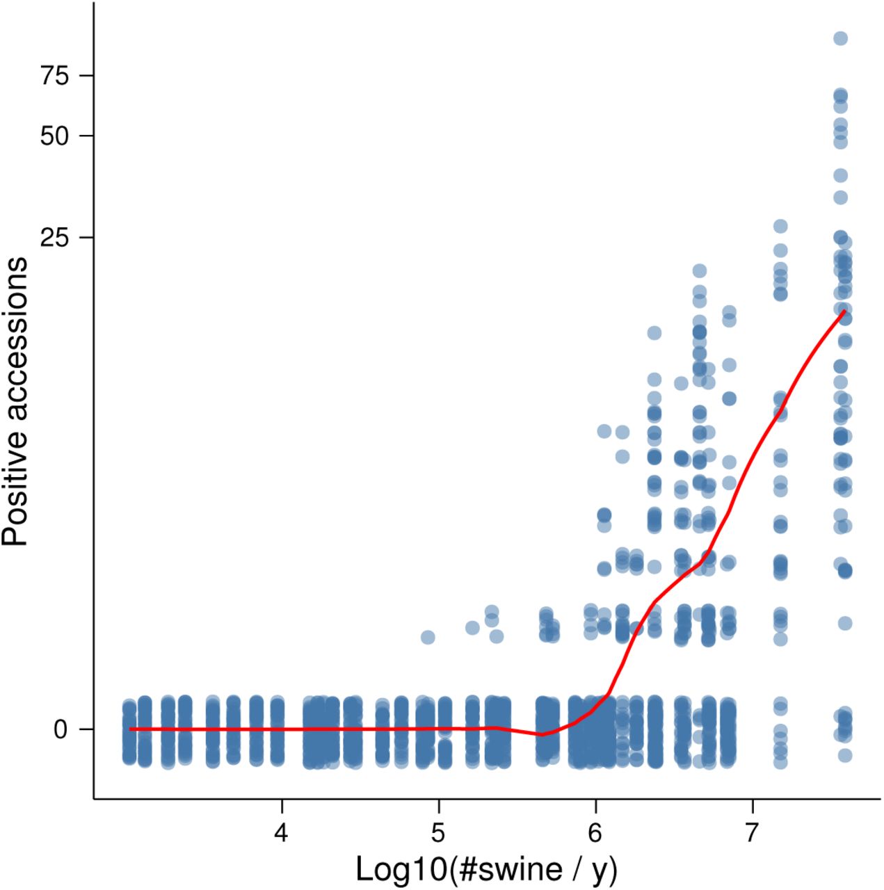
Fig. 4 displays the predicted and observed marginal relationships between flows and positive accessions for one of the models. Although our flow variables were based on the outcome of variable selection, they are not equivalent to any of the variables in the variable selection procedure and the data analysed here has a time dimension not present in the data used for variable selection. Thus to confirm the statistical significance of the within-state flows, we conducted a likelihood ratio test of the hypothesis that models lacking terms for within-state flow were sufficient. The test favoured rejection of models without within-state flows . Descriptive statistics for the variables in the models compared are in Supplementary Note 1.

Figure 4.

Transport flows were predictive of the number of new positive accessions. The line is a LOESS smoother of predicted values from the undirected model, where predictions were calculated for each observation by adding fixed effects and conditional modes of random effects. The points are the original data. To display their density, they have been made transparent and jittered along the y axis. The y axis was transformed using y = log(Positive accessions + 1).

Among those models containing flows, undirected models, which assumed that flows increased contact rates in both source and destination states, fit best, and directed models, which assumed that flows increased contact of susceptible farms in the destination state to infective farms in the origin state, fit worst (Table 2). However, the parameter estimates were generally similar for all of these models, with flows having an appreciable effect (Fig. 5).

Figure 5.

Parameter estimates for the transmission model. The estimates are not sensitive to the choice of interstate flow model, and flows have similar effect sizes to farm densities. Baseline risk refers to the parameter η, which determines the risk of infection when no infectives are present. The error bars represent 50-and 95-percent Wald confidence intervals. The scaled variables were divided by the interquartile ranges to make their effect estimates comparable. The interquartile ranges for week and the logarithm of farm density were 19.0 and 4.5. Those for the logarithm of undirected, directed, and internal (no interstate) transport flows were 4.5, 4.3, and 3.8.

Table 2.

Summary of models. The models chiefly differ by how contact is assumed to depend on flows. In the null model, denoted by none, contact was independent of flows. In the internal model, contact was a function of within-state flows. In the directed model, contact was a function of flows moving into a state and within-state flows. In the undirected model, contact was a function of within-state flows and both flows into and out of a state. The column “Fit η?” indicates whether we estimated the value of η, which corresponds to risk that is independent of the number of infective farms. The symbol θ denotes the dispersion parameter of the negative binomial response. The symbol σ denotes the standard deviation of the random effect of (geographic) state on transmission rates. The abbreviation d.f. is for degrees of freedom (i.e., the number of parameters estimated). ΔAIC gives the AIC (Akaike information criteria) of a model minus the lowest AIC of all models.

Discussion

We have estimated the effects of several features of state-level population structure on the time and location of PED outbreaks. We first found that cross correlations in the time series of positive accessions became more similar as transport flows and geographical closeness increase. Simulations confirmed that such a positive association can occur when the distribution of interstate contacts is distributed among farms in the same way among different pairs of states. We then screened several candidate predictors of the cumulative burden of PED and found the relevant ones to be total number of farms and swine balance-sheet variables. We finished by fitting a model that provides a hypothesis of how the balance-sheet variables identified as relevant may be affecting transmission via their relationship with transport flows of swine.

The hypothesis that transportation is associated with the risk of PED transmission is not new, but our analysis does provide a new argument in support of it as well as parameters for a model of spread via transportation based on field data. From Fig. 5 we have the estimate for the directed model that one factor in the average pairwise transmission rate from farms in one area to those in another increases with the annual transport flow raised to the power of about 3.2/4.3. In general, transmission rate parameters have a strong effect on the output of models of livestock disease spread and modellers must rely on expert opinion to set them.^{32, 33} Estimates such as ours may thus be key for determining what parameter values are consistent with past epizootics.

Such use of our parameter estimates requires that the associated models be clearly understood, and one possible source of confusion in our models is the meaning of undirected flows. We suggest interpreting directed flows as a model of transmission by movement of live animals and undirected flows as a model of transmission where the trucks, trailers, and transport personnel act as mechanical vectors of PEDV. For example, if a truck regularly moves animals from one group of farms to another, they might pick up the virus where they drop off the animals and drop off the virus where they pick up the animals just as frequently as the other way around. If trucks generally serve farms in one or two states, then each such mechanical-vector contact from one state to another must generally be reciprocated if we suppose that the number of trucks in each state is stable over time. Given a constant average shipment size, the rate of these contacts will be proportional to our undirected flows. We do not suggest interpreting the better fit of the undirected model (Table 2) as strong evidence that it is in general a better model for PED spread because we were only able to differentiate between directed and undirected flows between states, while a large part of all flow is within states. In summary, the directed and undirected models each imply their own mechanism of transmission, and those interested in using the parameters for later analyses should be aware of the difference between them.

Any consumers of the parameter estimates should also consider the limitations of the analysis producing them. One limitation of this study is that the transport flows used excluded transport to harvest plants, and such movements have been observed¹⁰ to result in the contamination of trailers. This limitation may in part explain the weakness of the correlation of flows with cross correlations. At any rate, the common assumption that movements of animals to slaughter represent a dead end for disease spread may well be invalid for PED, and more data about these movements and the sharing of trailers among farms could allow for estimation of any associated risks.

A related limitation is the coarseness and age of our flow estimates. In support of them being sufficiently informative, previous phylogeographic analysis³⁴ has found evidence that the same flow data we used was predictive of the movement of H1 influenza A virus among swine. This result suggests that in spite of ongoing change in the population structure of the swine herd the 2001 flow estimates have a relatively stable predictive value because the samples for that phylogenetic analysis came from years 2005–2010. Likewise, 2009 interstate flow estimates for the U.S. cattle herd were in general agreement with 2001 estimates.³⁵ Of course, updated flow estimated are desirable for future modelling.

The main limitation of this analysis is that flows are correlated with several other variables, and we cannot rule out that these other variables are the true drivers of the observed effect of flows. We have formulated our time series SIR model based on the relationship between flows and inventory. These two variables are closely related both because more swine are moving through the farms with larger inventory and because swine often have shorter residence times on larger farms, since larger farms tend to specialise on specific production stages. But if larger farms did not experience more PED outbreaks but only reported them with higher probability, that could provide a false signal that flows are associated with risk. A phylogeographic analysis or analysis of suitably structured epidemiological data could establish an association between flows and spread of PEDV that is not subject to such confounding.

Both the objectives, identifying variables relevant to the risk of infection, and challenges of our data analysis, uncertain reporting rates and many correlated candidate predictors, are common in epidemiological studies. Two reasonable steps toward such an objective are to assemble as many relevant explanatory variables as possible about reporting rates and measures of exposure based on prior scientific knowledge and then to determine if the available data support the conclusion that these variables are relevant. Our general contribution has been to provide a worked-out example of how variation in the structure of the population across a large scale may lead to the formulation of candidate variables with potential relevance to mechanisms of spread or reporting. We have also demonstrated the use of stability selection and regularised regression for the task of filtering out noise variables from a set of candidates. These examples may serve to provide analysts with new ideas about how to make the most efficient use of often limited epidemiological data, hopefully leading to more rapid understanding of transmission and how to stop it.

Methods

Data

The data on transport flows comes from a study by the USDA Economic Research Service,³⁶ and the PED case data are provided by the American Association of Swine Veterinarians. Both data sets are open and publicly available.

Percent decrease in pig litter was calculated as the difference in litter size between the 2013 and 2014 December through February estimates⁷ divided by the 2013 estimates and multiplied by −100.

Sixteen states had individual pig litter estimates, and a group average is reported for the other states. We assumed that the decreases for states in that group were close to the group average, which was 1 percent, and thus that those states had decreases less than 2 percent.

Simulation model

We use a discrete-time model in which the probability that a susceptible vertex i avoids becoming infected at the next time step is equal to exp (−β ∑_j≠i A_ijI_j), where β is the transmission rate, A_{i j} is the weight of the edge pointing to vertex i from vertex j, and I_j is an indicator variable equal to one if vertex j is infected and equal to zero otherwise. The edge weight A_{i j} represents the amount of infective material that vertex i may receive from vertex j and the transmission rate is the expected number of infections per unit of this infective material. In the case of livestock diseases, we might think of the edge weight as proportional to the number of animals moved from one farm to another and the transmission rate as the rate at which the probability of a farm avoiding infection decreases for a given number of animals introduced from an infective farm.

We set the transmission rate in terms of an R₀ baseline parameter, which we define as β(N − 1), where N is the number of vertices in the network. Thus we do not change the transmission rate as the number of edges is changed, which we find makes the results easier to interpret.

For simplicity, we assume infective vertices recover in one time step. To allow for highly stochastic dynamics without extinction, we assume that all vertices have some constant probability of infection from vertices outside of the simulated population. We describe this parameter in terms of the expected number of introduced infections, which is equal to the number of vertices in the network times the per-time-step probability of any one of them being infected from an external source.

We calculate lag-1 cross correlation using a window of 500 time steps that follows a warm-up period of 500 time steps that allowed the model to reach a stationary distribution. All simulations began with a completely susceptible population at the beginning of the warm-up.

Wiring schemes

The vertex sets corresponding to each of the partitions are kept fully connected to because fully connected networks are highly symmetric, and thus the sets of unique cut sets are easier to systematically explore. The wiring schemes differ in which edges are added as we increase the size of the cut set, which is most easily described in terms of non-zero elements of the adjacency matrix of the network. We begin with a block-diagonal adjacency matrix where the blocks on the diagonal contain weights of within-partition edges and the complementary blocks contain the weights of edges in the cut set. We consider only undirected networks so a particular cut set can be described in terms of one of the cut-set blocks. In the balanced scheme, the degree distribution (i.e., the probability mass distribution for the number of neighbours of each vertex) of the two partitions is kept as balanced as possible. Thus cut-set edges are added by forming bands on the diagonal of the block of increasing width. In the unbalanced scheme, the degree distribution is kept as unbalanced as possible. Thus cut-set edges are added by filling in the cut-set block column by column. Consequently, one of the partitions contains vertices with many cut-set members incident to them, which we refer to as hubs. In the reciprocally-unbalanced scheme, cut-set edges are added by filling in columns and rows in an alternating manner. Thus hubs appear in each partition in an alternating manner.

In all schemes, we distribute the total weight of cut-set edges evenly among them. The total flow is set to n²c, where n is the size of each of the partitions and c is a tuning parameter we refer to as a capacity factor. The weight of edges outside of the cut set was fixed at 1. Thus when varying the number of edges in the cut set, the modularity statistic Q²⁸ remains unchanged. This invariance makes our schemes similar to the previously introduced idea of different mixing styles.³⁷

Regularised regression and stability selection

Many states had no confirmed positive accessions (Fig. 1b) such that the case counts appear to be a mixture of zeroes and a right-skewed distribution of counts. Thus we chose to fit the data to a hurdle model in which the probability of a state having a confirmed case and the number of positive accessions, given that there is at least one case in the state, are described by separate regression models. We used binomial generalised linear models for the probability responses and a least-squares linear model for the response of the log of positive accessions. Predictors were put onto the same scale by dividing by standard deviations.

The elastic net penalty includes a tuning parameter, denoted by α, that determines the extent to which groups of correlated variables are selected together. We set α to 0.8 to allow for highly correlated variables to be grouped for selection while still keeping the total number of selected variables small.

The choice α = 0.8 was made subjectively, but we checked that the results were not sensitive to this choice by also looking at the results with α ∈{0.01,0.2, 0.5,1}. For α ≠ 1, only additional balance sheet variables were selected for all models. When α = 1, inventory and resource region 4 were selected as predictors of both litter rate decrease and total positive accessions, and no variables were selected as predictors of whether any positive accessions occurred. We consider these aberrations likely to be an artefact of correlations among predictors, as single members of correlated groups can be selected somewhat arbitrarily when α = 1.

For stability selection, we used 1,000 subsamples of 63.2 percent of the full data sets (the same percentage that would appear in large bootstrap samples of a data set). The set of selected variables was chosen by using a threshold parameter π_thr of 0.6 and choosing the regularisation parameter λ to select as many variables as possible while keeping the per-comparison error rate (i.e., the probability that any one variable is incorrectly selected) below 0.05. The results of stability selection are not usually sensitive to the choice of π_thr as long as it is between 0.6 and 0.9. The error rate is only guaranteed to hold under the restrictive assumption of exchangeability for the selection probability of all noise variables, but numerically it has been found to be accurate even when this assumption was most likely not satisfied.³⁰ Although we cannot guarantee similar accuracy for our data set, we propose that controlling the nominal error rate provides a reasonable criteria for identifying the candidate variables that are most likely to be relevant.

Regression models of transmission rates

The transmission model is integrated within a regression model by having the expected number of infectives in state i at week t + 1, E(I_i,_t+1) follow where β_i,_t is the transmission rate for state i at time t, w_i, _j is the weight for the influence of infectives in state j on susceptibles in state i, η is parameter that determines the influence of other sources of infection, α determines the power by which the expected number of transmissions grows with these risks, and S_i,_t is the number of susceptibles in state i at week t. We set , where N_i is the number of farms in state i from the 2002 Census of Agriculture.³⁸ This model is a variant of the time series SIR (susceptible–infective–recovered) model.³⁹ Supplementary Note 4 discusses some of the assumptions and data we used for this model.

Our calculation of S_i,_t assumes that all farms were susceptible to infection at the beginning of the epizootic and that farms pass on to an immune state following infection. The assumption of complete susceptibility seems reasonable for the United States given the absence of previous reports of PED and the high frequency of high-mortality outbreaks that followed the first reported outbreak.⁹ Although PED has been observed to reoccur on a farm,²⁶ that observation was a newsworthy event⁴⁰ and it followed a 6-month interval of normal operations. Thus the assumption of immunity over the 38 week period that we analyse seems reasonable.

Our transmission rate β_i,_t in Eq. 1 takes the form where the c_i are unknown parameters that we estimate, Z_i represents state-level random effects, d_i is a state-level summary statistic of the county-level farm density from the 2007 Census,⁴¹ and f_i is value characterising the average flow of swine through individual farms in state i. c₁ allows the transmission rate to vary seasonally, which has been proposed as an explanation for why most positive accessions occurred in the fall and winter. For the summary statistic d_i, we used the median county-level density among counties with any farms in the state. The results were not sensitive to using this statistic versus others such as the overall median or mean. d_i is multiplied by because that led to the greatest correlation between the density and flow terms on the logarithmic scale, and we wished to as much as possible separate the estimated effects of flows with those of farm density. It also allowed us to see whether density-dependent transmission⁴² is suggested by the data, which would have corresponded to estimates (ĉ2,ĉ3) ≈ (1,0).

The characteristic flows f_i in Eq. 2 and the weights w_i in Eq. 1 are calculated in various ways to model the rate of contact of a susceptible farm with infected farms in various scenarios. We make the derivations assuming α = 1, and values of α below 1 can be understood as capturing the effects of infective farms being clustered together in the contact network. Let F_i, _j be the number of swine shipped to farms in state i from farms in state j per year. In the directed model, only farms receiving animals are at risk for infection. Then, omitting the time subscripts for simplicity, susceptible farms in state i are infected at a rate proportional to ∑_j F_i, _j(N_iN_j)⁻¹I_j, or , where f_i = ∑_j F_i, _j and . In the undirected model, both farms sending and farms receiving animals may be at risk, and susceptible farms in state i are infected at a rate proportional to ∑_j(F_i, _j + F_j,_i)(N_iN_j)⁻¹I_j, which implies that f_i = ∑_j F_i, _j + F_j,_i and .

In the internal model, both farms sending and receiving animals may be at risk, but transmission associated with flows only occurs within a state. Thus susceptible farms in state i are infected at a rate proportional to , which implies that f_i = 2F_i,_i and w_i, _j = δ_i, _j, Kronecker deltas. Comparison of the fit of this model with the directed or undirected models allows any effects of between-state transmission to be seen. The internal model also includes in the case that c₃ = 0 a null model which has no flows in it, which we use in a likelihood ratio test of the hypothesis that flows have no effect on transmission rates.

The values of F_i, _j, when i ≠ j, come directly from the estimates³⁶ of interstate flows. We estimated within-state flows in two ways. In the first, a demand for pigs was calculated for state i from 2002 sales³⁸ of finish-only and nursery operations plus the deaths reported in the 2001 balance sheet.⁴³ Internal flow, F_i,_i, was estimated as the this demand less imports, ∑_{j, j≠i} F_i, _j. In the second method, F_i,_i was estimated as the combined sales of farrow-to-wean, farrow-to-feeder, and nursery operations less exports, ∑_j,_i≠jF_j,_i. For most states with large inventories, the logarithms of these two estimates were similar relative to estimates from other states, and we averaged the log-transformed estimates to generate a single estimate. For the other states, one of the estimates was negative, and we simply used the positive estimate. We suspect the negative estimates and the difference between the positive estimates stem in part from us not being able to use 2001 sales data or to account for internal supplies of and demand for breeding animals. Coarse as these estimates may be, it still seems reasonable to us that they will permit detection of large, state-level associations.

To fit the model, we form a linear predictor of logE(I_i,_t+1) by substituting Eq. 2 into Eq. 1 and taking logarithms to obtain

We fit this model to data from all 48 contiguous states with the assumption that the observed positive accessions I_i,_t+1 have a negative binomial distribution with an unknown, but constant, dispersion parameter which we denote with θ. This parameter is related to the variance by Var(I_i,_t+1) = E(I_i,_t+1)[1 + E(I_i,_t+1)/θ]. We assume that the random effect Z_i is normally distributed. Then the likelihood is fully specified. We calculate marginal likelihoods with the Laplace approximation and numerically find the parameters that maximise it. In some cases we fixed η to 0.5, which allowed the model to be fully fit with both the lme4⁴⁴ and glmmADMB⁴⁵ packages in R.⁴⁶ To make sure our results were not sensitive to η = 0.5, we used R’s optimise function to find the value of η in [0,5] with highest likelihood.

We performed several diagnostic checks of our fits, including checking for signs of nonlinearity with partial residual plots and for signs of temporal autocorrelation in the residuals. We also verified that the flows term is significant in models lacking random effects, and after excluding any data points with dfbetas⁴⁷ above 0.2.

Software

We used R⁴⁶ for most of this work. The key contributed packages used were c060,⁴⁸ igraph,⁴⁹ glmmADMB,⁵⁰ glmnet,⁵¹ ggplot2,⁵² lme4,⁵³ and vegan.⁵⁴ We performed the edge bundling for Figs. 1c and 1d using JFlowMap.⁵⁵ Code to reproduce the results is archived on the web,⁵⁶ and has been developed to run in Docker⁵⁷ containers for enhanced reproducibility. Thus, after installing one open-source software package on their personal computer, interested readers may quickly repeat our analysis, examine intermediate results, perform their own diagnostics, and extend this work.

Author contributions statement

S.B. and E.O. designed the study and drafted the manuscript. E.O. conducted the analyses. H.S. reviewed the veterinary subject matter of the manuscript.

Acknowledgements

This work was supported by DHS Contract # HSHQDC-12-C-0014; the RAPIDD Program of the Science & Technology Directorate, Department of Homeland Security; and the Fogarty International Center, National Institutes of Health. The content is solely the responsibility of the authors and does not necessarily reflect the official views of the National Institutes of Health or the Department of Homeland Security.

We thank John Korslund for useful feedback on veterinary subject matter. We thank John Drake and Chris Dibble for comments that improved the clarity of the writing.