Learning from heterogeneous data sources: an application in spatial proteomics

Abstract

Sub-cellular localisation of proteins is an essential post-translational regulatory mechanism that can be assayed using high-throughput mass spectrometry (MS). These MS-based spatial proteomics experiments enable to pinpoint the sub-cellular distribution of thousands of proteins in a specific system under controlled conditions. Recent advances in high-throughput MS methods have yielded a plethora of experimental spatial proteomics data for the cell biology community. Yet, there are many third-party data sources, such as immunofluorescence microscopy or protein annotations and sequences, which represent a rich and vast source of complementary information. We present a unique transfer learning classification framework that utilises a nearest neighbour or support vector machine system, to integrate heterogeneous data sources to considerably improve on the quantity and quality of sub-cellular protein assignment. We demonstrate the utility of our algorithms through evaluation of five experimental datasets, from four different species in conjunction with three different auxiliary data sources to classify proteins to tens of sub-cellular compartments with high generalisation accuracy. We further apply the method to a experiment on pluripotent mouse embryonic stem cells to classify a set of previously unknown proteins, and validate our findings against a recent high resolution map of the mouse stem cell proteome. The methodology is distributed as part of the open-source Bioconductor pRoloc suite for spatial proteomics data analysis.

1 Introduction

Cell biology is currently undergoing a data-driven paradigm [1] shift. As highlighted by [2], the experimental tools of molecular biology, imaging and biochemistry enable cell biologists to track the complexity of many fundamental processes such as signal transduction, gene regulation, protein interactions and sub-cellular localisation. They note that “with the culmination of ’omic technologies, the molecular and cellular parts lists of cells are known, quantifiable, and increasingly readily available in electronic databases. This remarkable success at the same time signifies that biology has irreversibly changed to a data rich science.” Over the last decade, there has been a dramatic growth in data, both in terms of size and heterogeneity. Coupled with this influx of experimental data, databases such as Uniprot [3] and the Gene Ontology [4] have become more information rich, providing valuable resources for the community. The time is ripe to take advantage of complementary data sources in a systematic way to support hypothesis-and data-driven research. Indeed, one of the biggest challenges in computational biology is how to meaningfully integrate heterogenous data; transfer learning, a paradigm in machine learning, is ideally suited to this task.

Transfer learning has yet to be fully exploited in computational biology and is still a growing field within the machine learning community. To date, various data mining and machine learning tools, in particular classification algorithms have been widely applied in many areas of biology [5]. A classifier is trained to learn a mapping between a set of observed instances and associated external attributes (class labels) which is subsequently used to predict the attributes on data with unknown class labels (unlabelled data). In transfer learning, one has a primary task which one wishes to solve, and associated primary data which is typically expensive, of high quality and targeted to address a specific question about a specific biological system/condition of interest. While standard supervised learning algorithms seek to learn a classifier on this data alone, the general idea in transfer learning is to complement the primary data by drawing upon a auxiliary data source, from which one can extract complementary information to help solve the primary task. The secondary data typically contains information that is related to the primary learning objective, but was not primarily collected to tackle the specific primary research question at hand. These data can be heterogenous to the primary data and are often, but not necessarily, cheaper to obtain and more plentiful but with lower signal-to-noise ratio.

There are several challenges associated with the integration of information from auxiliary sources. If the primary and auxiliary sources are combined via straightforward concatenation the signal in the primary can be lost through dilution with the auxiliary due to the plentiful and often lower signal-to-noise ratio found in the auxiliary for the primary task. Feature selection can be used to extract the attributes with the most distinct signals, however the challenge still remains in how to combine this data in a meaningful way. Data heterogeneity is also a challenge; combining data that exist in different data spaces is often not straightfor-ward and different data types can be sensitive to the classifier employed, in terms of classifier accuracy.

In one of the first applications of transfer learning Wu and Dietterich [6] used a k-nearest neighbours (k-NN) and support vector machine (SVM) framework for plant image classification. Their primary data consisted of high-resolution images of isolated plant leaves and the primary task was to determine the tree species given an isolated leaf. An auxiliary data source was available in the form of dried leaf samples from a Herbarium. Using a kernel derived from the shapes of the leaves and using the auxiliary transfer learning framework described in [6], Wu and Dietterich showed that when primary training data is small, training with auxiliary data improves classification accuracy considerably. There were several limitations in their methods: firstly, the data sources in the k-NN transfer learning (TL) classifier could only be weighted by data source and not on a class-by-class basis, and secondly in the SVM framework the primary and auxiliary data were expected to have the same cardinality and lie in the same data space. Here, we present an adaption and significant improvement of this framework and extend the usability of the method by (i) incorporating a multi-class weighting schema in the k-NN TL classifier, and (ii) by allowing the integration of primary and auxiliary data with different cardinality in the SVM schema to allow the integration of heterogenous data types. We apply this framework to the task of protein sub-cellular localisation prediction from high resolution mass spectrometry (MS)-based data. While we demonstrate algorithmic usage for the spatial proteomics community the framework can be applied in many areas of computational biology.

Spatial proteomics, the systematic large-scale analysis of a cell’s proteins and their assignment to distinct sub-cellular compartments, is vital for deciphering a protein’s function(s) and possible interaction partners. Eukaryotic cells are divided into sub-cellular niches, which include organelles and macro-molecular complexes of proteins which represent specialised compartments with unique and dedicated functions [7]. Knowledge of where a protein spatially resides within the cell is covetable to biologists as it not only provides the physiological context for their function but also plays an important role in furthering our understanding of a protein’s complex molecular interactions e.g. signalling and transport mechanisms, by matching certain molecular functions to specific organelles. It has been shown that there is a significant correlation between aberrantly localised proteins and many human diseases as diverse as Alzheimer’s disease, kidney stones and cancer [8], further highlighting the importance of protein localisation and the role that spatial proteomics may play in developing new platforms for therapeutic intervention.

There exist a number of sources of information which can be utilised to assign a protein to a sub-cellular niche. These range from high quality data produced from experimental high-throughput quantitative MS-based methods and imaging data, to freely available data from repositories and amino acid sequences. In the field of high-throughput quantitative proteomics, many modern experimental designs and multivariate data analysis methods have been developed which involve the creation of single or multiple fractions of a cell lysate to quantify and identify the protein content of a population of potentially heterogeneous cells to permit the assignment of proteins to tens of different sub-cellular niches at the whole proteome level [9]. Other approaches consider more global distribution patterns of proteins in sub-cellular niches using defined enrichment patterns, for example the Localisation of Organelle Proteins by Isotope Tagging (LOPIT) pioneered by Dunkley et al [10] and Protein Correlation Profiling (PCP) by Foster et al [11] in 2006.

These methods involve gentle cell lysis followed by several rounds of differential centrifugation or gradient-based ultra-centrifugation to separate the cell content as a function of its density. Several fractions across the gradient are then collected and their respective protein complements are identified and quantified by high resolution MS. Protein distributions are then determined by measuring their relative abundance across the fractions employed. The resulting data from these methods is in the form of a matrix where the rows represent proteins and the columns contain the relative abundance of each protein in each fraction along the sub-cellular fractionation gradient. Proteins with similar organelle residency will share similar distribution profiles characteristic of the sub-cellular compartment with which they are associated [12]. These approaches have been heavily utilised to gain information about the sub-cellular location of proteins in numerous species, for example Arabidopsis [10, 13, 14, 15, 16, 17], Drosophila [18], yeast [19], human cell lines [20, 21], mouse [11, 22] and chicken [23]. Such analyses has resulted in large-scale data sets to enable the simultaneous assignment of thousands of proteins to multiple sub-cellular locations.

Based on the distribution of a set of known genuine organelle residents, termed marker proteins, pattern recognition and machine learning (ML) methods can be used to match and associate the distributions of unknown residents to that of one of the markers. Traditional spatial proteomics relies extensively on reliable organelle markers and multivariate statistical and supervised ML methods for high-throughput reliable proteome-wide localisation prediction [24]. To date, classification had been tackled using a number of popular supervised ML algorithms, for example, support vector machines (SVMs) [25], the k-nearest neighbours (k-NN) algorithm [16], random forest [26], naive Bayes [15], neural networks [27], and other classic multivariate statistical methods such as partial-least squares discriminant analysis [10], [18], [23], and the χ² metric [20, 11].

Computational development applied to MS-based protein-organelle association are a recent development, but the computational determination of protein localisation using in silico data is an established bioinformatics challenge (reviewed in [28, 29, 30]). Many methods have been developed to predict protein localisation from amino acid sequence features e.g. amino-acid composition information (e.g. [31, 32, 33, 34, 35, 36, 37]), localisation signals and motifs relevant to protein sorting (e.g. [38, 39, 40, 41, 42, 43, 44, 45]). Annotation-based prediction methods have also been widely used that use information about functional domains (e.g. [46, 47]), protein-protein interaction (e.g. [48, 49, 50]) and Gene Ontology (GO) [4] terms (e.g. [51, 52, 53, 54]). Although not all proteins in GO are reliably annotated, for example, according to the 2015 03 release of UniProtKB [3] the human, mouse, Drosophila melanogaster and Arabidopsis thaliana proteomes have less than 14%, 14%, 6% and 13% experimentally-verified GO CC sub-cellular annotations, in each proteome respectively.

Despite improvements in generalisation accuracy of sequence-and annotation-based classifiers, a fundamental problem concerns the biological relevance and ultimate utility to cell biology of such predictors. Protein sequences and their annotation do not change according to cellular condition or cell type, whereas protein localisation does. Furthermore, this type of data does not adequately describe the range of mechanisms via which a particular protein may reside in a particular organelle. Not all protein sequences contain motifs or exhibit compositional properties indicative of organelle residency. This considerable body of ML research into the prediction of protein-organelle association from annotated protein sequence has yet to be exploited within organelle proteomics experiments. Despite the inherent limitations of using in silico data to predict dynamic cell- and condition-specific protein properties, transfer learning [6, 55] may allow the transfer of complementary information available from these data to classify proteins in experimental proteomics datasets. Transfer learning has been used to predict sub-cellular localisation from in silico data sources such as GO terms and Chou’s pseudo amino-acid composition [52, 53, 54], but no framework has yet been developed to allow the integration of experimental data and third-party sources. It is well documented that training ML models on multiple related data sources can lead to higher generalisation accuracies than those obtained on each data set individually [25, 56, 57, 58]. Other possible data sources include protein-protein interaction partners (which must share sub-cellular localisation in order to interact), imaging data, for example data available from such projects as the Human Protein Atlas [59], and other annotation sources.

Here, we present a new transfer learning framework, inspired by Wu and Dietterich’s classic inductive transfer learning framework [6]. The primary task is protein localisation prediction from MS-based quantitative proteomics datasets, and we exploit a secondary auxiliary data source to improve classification. We use, among others, Gene Ontology Cellular Compartment (GO CC) terms as an auxiliary data source, to improve upon the classification of experimental and condition-specific sub-cellular localisation predictions from MS-based quantitative proteomics data in an organelle specific manner. Using the k-Nearest Neighbour (k-NN) and support vector machine (SVM) algorithms in a transfer learning framework we find that when given data from a high quality MS experiment, integrating data from a second less information rich but more plentiful auxiliary data source directly in to classifier training and classifier creation results in the assignment of proteins to organelles with high generalisation accuracy. Five experimental MS LOPIT datasets, from four different species, were employed in testing the classifiers. We further show the flexibility of the pipeline through testing two other auxiliary data sources; (1) tagging-based sub-cellular imaging data [59], and (2) sequence and annotation features (see table 1) obtained from a correlation-based feature selection [60] on the input features used for the classifier YLoc [61, 62]. The results obtained demonstrate that this transfer learning method outperforms a single classifier trained on each single data source alone and on an class-by-class basis, high-lighting that the primary data is not diluted by the auxiliary data. A new transfer learning framework for the integration of heterogeneous data sources is proposed. This methodology forms part the open-source open-development Bioconductor [63] pRoloc [64] suite of computational methods available for organelle proteomics data analysis.

Table 1:

A summary of the types of features considered in training and building Briesemeister et al’s YLoc classifier.

2 Materials and methods

2.1 Data sources

2.1.1 Primary data

Five datasets, from studies on Arabidopsis thaliana [10, 16], Drosophila embryos [18], human embryonic kidney fibroblast cells [21], and mouse pluripotent embryonic stem cells (E14TG2a) (unpublished) were collected using the standard LOPIT approach as described by Sadowski et al. [13]. In the LOPIT protocol, organelles and large protein complexes are separated by iodixanol density gradient ultracentrifugation. Proteins from a set of enriched sub-cellular fractions are then digested and labelled separately with iTRAQ or TMT reagents, pooled, and the relative abundance of the peptides in the different fractions is measured by tandem MS. The number of measurements obtained per gradient occupancy profile (which comprises of a set of isotope abundance measurements) is thus dependent on the reagents and LOPIT methodology used.

The first Arabidopsis thaliana dataset [10] on callus cultures employed dual use of four isotopes across eight fractions and thus yielding 8 values per protein profiles. The aim of this experiment was to resolve Golgi membrane proteins from other organelles. Gradient-based separation was used to facilitate this, including separating and discarding as much nuclear material as possible during a pre-centrifugation step, and carbonate washing of membrane fractions to remove peripherally associated proteins, thereby maximising the likelihood of assaying less abundant integral membrane proteins from organelles involved in the secretory pathway.

The second Arabidopsis thaliana dataset on whole roots is one of the replicates published by Groen et al. [16], which was set up to identify new markers of the trans-Golgi network (TGN). The TGN is an important protein trafficking hub where proteins from the Golgi are transported to and from the plasma membrane and the vacuole. The dynamics of this organelle are therefore complex which makes it a challenge to identify true residents of this organelle. For each replicate, sucrose gradient fractions were subjected to a carbonate wash to enrich for membrane proteins and four fractions were iTRAQ labelled. Following MS the resultant iTRAQ reporter ion intensities for the four fractions were normalised to six ratios and then each proteins abundance was further normalised across its six ratios by sum. In Groen’s original experiment the iTRAQ quantitation information for common proteins between the three different gradient were concatenated to increase the resolution of the TGN [25].

The aim of the Drosophila experiment [18] was to apply LOPIT to an organism with heterogeneous cell types. Tan et al. were particularly interested in capturing the plasma membrane proteome (personal communication). There was a pre-centrifugation step to deplete nuclei, but no carbonate washing, thus peripheral and luminal proteins were not removed. In this experiment four isotopes across four distinct fractions were implemented and thus yield four measurements (features) per protein profile.

The human dataset [65, 21] was a proof-of-concept for the use of LOPIT with adherent mammalian cell culture. Human embryonic kidney fibroblast cells (HEK293T) were used and LOPIT was employed with 8-plex iTRAQ reagents, thus returning eight values per protein profile within a single labelling experiment. As in the LOPIT experiments in Arabidopsis and Drosophila, the aim was to resolve the multiple sub-cellular niches of post-nuclear membranes, and also the soluble cytosolic protein pool. Nuclei were discarded at an early stage in fractionation scheme as previously described, and membranes were not carbonate washed in order to retain peripheral membrane and lumenal proteins for analysis.

The E14TG2a embryonic mouse dataset (unpublished) also employed iTRAQ 8-plex labelling, with the aim of cataloguing protein localisation in pluripotent stem cells cultured under conditions favouring self-renewal. In order to achieve maximal coverage of sub-cellular compartments, fractions enriched in nuclei and cytosol were included in the iTRAQ labelling scheme, along with other organelles and large protein complexes as for the previously described datasets. No carbonate wash was performed.

All datasets are freely distributed as part of the Bioconductor [63] pRolocdata data package [64].

2.1.2 Auxiliary data

The Gene Ontology (GO) project provides controlled structured vocabulary for the description of biological processes, cellular compartments and molecular functions of gene and gene products across species [4]. For each protein seen in every LOPIT experiment the protein’s associated Gene Ontology (GO) cellular component (CC) namespace terms were retrieved using the pRoloc package [64]. Given all possible GO CC terms associated to the proteins in the experiment we constructed a binary matrix representing the presence/absence of a given term for each protein, for each experiment.

Human Protein Atlas

The Human Protein Atlas [66] (version 13, released on 11/06/2014) was used as an auxiliary source of information to complement the human LOPIT dataset. The sub-cellular atlas provides protein expression patterns on a sub-cellular level using immunofluorescently staining for human U-2 OS cells. We used the hpar Bioconductor package [67] to query the atlas. The data was encoded as a binary matrix describing the localisation of 670 proteins in 18 sub-cellular localisations that have been supportively identified.

YLoc Classifier Features

YLoc [61, 62] is an interpretable web sever developed by Briesemeister and co-workers for the prediction of protein sub-cellular localisation. The YLoc classifier uses features derived from numerous data sources from both sequence and annotation. A summary of the features included in the YLoc classifier are shown in Table 1. These features provide a source of complementary auxiliary data for the high quality MS based datasets described in 2.1.1. To use these features as an auxiliary source of information, a large-scale correlation-based feature selection (CFS) approach [60], as described in [61, 62], was used with the markers from the E14TG2a mouse dataset to find the set of the most important features.

The definition of primary and auxiliary is not defined algorithmically, by the quality or the size of the data but rather by the data and question at hand. For example, here LOPIT was considered the primary data because it represented the experiment of interest that was to be complemented by the imaging data. In fact, from an algorithm point of view, primary and auxiliary are reciprocal.

2.1.3 Markers

Spatial proteomics relies extensively on reliable sub-cellular protein markers to infer proteome wide localisation. Markers are proteins that are defined as reliable residents and can be used as reference points to identify new members of that sub-cellular niche. Here, marker proteins are selected by domain experts through careful mining of the literature. Markers for each LOPIT experiment were specific to the system under study and conditions of interest and are distributed as part of the Bioconductor [63] pRoloc package [64].

2.2 Incorporating auxiliary data

2.2.1 Notation

The primary MS-based experimental datasets P consist of multivariate protein profiles. The auxiliary data A is a presence/absence binary matrix of Gene Ontology Cellular Compartment (GO CC) terms. Data are annotated to either (i) a single known organelle (labelled data), or (ii) have unknown localisation (unlabelled data). Thus we split P and A into labelled (L) and unlabelled (U) sections such that P = (L^P, U ^P) and A = (L^A, U ^A).

The labelled examples for P and A are represented by L^P = {(x_l, y_l) |l = 1, …, |L^P| where x_l ∈ ℝ^S, and L^A = {(v_l, y_l) |l = 1, …, |L^A| where v_l ∈ ℝ^T. Thus each l^th protein is described by vectors of S and T features (generally, S ≪ T), for P and A respectively. Each dataset shares a common set of proteins that is annotated to one of the same y_l ∈ C = 1, …, C sub-cellular classes, where |C|∈ℕ is the total number of sub-cellular classes. Unlabelled data, U ^P and U ^A are represented by U ^P = x_u u = 1, …, |U ^P |where x_u ∈ ℝ^S and U ^A = v_u |u = 1, …, |U ^A |} where v_u ∈ ℝ^T, respectively.

The labelled data for the i^th organelle class, with N_i indicating the number of proteins i for the i^th organelle class, is given for P by and for A by . The labelled dataset of all available proteins over the |C| different sub-cellular classes is given for P by and for A by .

2.2.2 Transfer learning using a k-nearest neighbours framework

We adapt Wu and Dietterich’s [6] classic application of inductive transfer using experimental quantitative proteomics data as the primary source (P) and GO CC terms as the auxiliary source (A). We aim to exploit auxiliary data to improve upon the sub-cellular classification of proteins found in MS-based LOPIT experiments in an organelle specific way, using the baseline k-nearest neighbours (k-NN) algorithm in a transfer learning framework.

In k-NN classification, an unknown example is classified by a majority vote of its labelled neighbours, with the example being assigned to the class most common among its k nearest neighbours. Independent of the transfer learning classifier we compute the best k for each data source for values k ∈ {3, 5, 7, 9, 11, 13, 15} through an initial 100 rounds of 5-fold cross-validation using each set of labelled training data for P and then independently for A (as implemented in pRoloc). We denote by k_P the best k for P, and by k_A the best k for A.

Having obtained the best k for each data source, the transfer learning algorithm works as follows. For the u^th protein (x_u, v_u) we wish to classify in U, we start by finding the k_P and k_A labelled nearest neighbours for x_u and v_u in L^P and L^A, respectively. Denote these sets and . We then define the vectors and to contain counts for each class in the sets of nearest neighbours; that is,

For each protein, let and be normalized vectors with elements summing to 1 and representing the distribution of classes among the sets of nearest neighbours for each protein. Finally, let and .

To include both the primary and auxiliary data in the set of potential neighbours we took a weighted combination of the votes in NN^P and NN^A for each sub-cellular class. Class weights are defined by the parameter vector θ^T = (θ₁, …, θ_|C|) with values chosen by optimisation through a prior 100 independent rounds of 5-fold cross-validation on a separate training partition of the labelled data. For the u^th unknown protein (x_u, v_u) in U, the voting scores for each class i ∈ C are calculated as and the protein is assigned to the class c ∈ C maximizing V (i)

The class weights θ_i in equation 1 control the relative importance of the two types of neigh-bours for each class i ∈ C. This differs from Wu and Dietterich’s [6] original approach as they only weight the data sources and not the classes and the data sources. In this paper we select each class weight θ_i from the set ; however, the algorithm allows us to use any real-valued θ_i ∈ [0, 1]. If θ_i = 1, then all weight is given to the primary data in class i and only primary nearest neighbours in class i are considered. Similarly, if θ_i = 0, then all weight is given to the auxiliary data in class i and only auxiliary nearest neighbours in class i are considered. If 0 < θ_i < 1 then a combination of neighbours in the primary and auxiliary data sources is considered.

2.2.3 Transfer learning using a SVM framework

Linear programming SVMs

The method is based on the use of the linear programming formulation of the SVM (lpSVM). This formulation promotes classifiers that are sparse, in the sense that where possible only a few parameters obtained through training are non-zero; for a detailed introduction see Mangasarian [69].

We begin by describing the standard lpSVM used for classical two-class classification problems with a single labelled training set. We use the multiple-class version of this approach with the individual primary and auxiliary sets P and A as a comparison later in the paper; we present the method here assuming that the primary set P is being used and can be set up as a binary classification problem; for example, we might wish to predict whether or not a protein should be assigned to a single specified sub-cellular class. For binary classification problems with class labels y ∈ {+1, −1}, and given labelled data L^P = {(x_l, y_l)|l = 1, …, m} where m = |L^P | the classifier takes the form where f is the latent function

Here, K^P is a kernel (Shawe-Taylor and Cristianini [70]) associated with the primary data and and b are parameters determined by training.

For any vector x^T = (x₁, …, x_n) let |.|₁ denote the 1-norm

The training algorithm requires that we solve the linear programme such that for each i = 1, …, m and α_P, ξ ≥0.¹ The parameters ξ and C act in the same way as the corresponding parameters in the standard SVM: ξ contains the slack variables allowing some examples to be misclassified, and C controls the extent to which such misclassifications are penalized during training.

Transfer learning for binary classification

Once again we adapt the method of Wu and Dietterich [6] to our problem. The original method requires adaptation as it is designed for data having two important differences compared with ours. First, it does not require examples in the labelled data sets L^P and L^A to be in correspondence and for corresponding training examples to share the same label. Second it assumes that P and A share the same number of features. While the first of these differences is easily dealt with as our data is a special case that is already covered, the second is more problematic. If we now introduce the labelled auxilliary data L^A = {(v_l, y_l)| l = 1, …, m} a direct application of the approach in [6] requires us to evaluate kernels of the form K(x, v). As P and A contain data with different numbers of features this presents a problem for any SVM-type method, as kernels are usually required to satisfy the Mercer conditions (Mercer [71]), one of which is that they are symmetric, such that K(x, x′) = K(x′, x). While research on the use of asymmetric kernels has appeared—see for example [72]—even if we relax this requirement a kernel is essentially a measure of the similarity of its arguments, and the question arises of how one might sensibly measure the similarity of a protein profile with a presence/absence vector of GO CC terms. This problem does not arise with Wu and Dietterich’s data as the two sets they use have the same dimension and are derived in a way that makes measuring similarity straightforward.

We therefore simplify the original method as follows. We maintain the machinary employed above for the primary data, and introduce a separate kernel K^A and parameter vector α_A for the auxilliary data. A vector to be classified now contains both a protein profile x and a GO vector v. The latent function becomes and training requires us to solve the linear program such that for each i = 1, …, m and a_P, a_A, ξ ≥ 0.

Note that this differs from the method of Multiple Kernel Learning (MKL) (Lanckriet et al. [73], Gönen and Alpaydin [74]) in that in MKL the single kernel K is replaced in the usual SVM formulation by a weighted sum of kernels where d_i ≥ 0 and . The d_i are then included with α and b in a more involved constrained optimisation problem. Our approach has the advantages that it remains a straightforward linear program and in fact introduces fewer constraints on the form of the latent function f.

Throughout our experiments we used for K^P and K^A the Gaussian kernel where ||.|| denotes the 2-norm . We optimized over the value of C, and also separate values γ_P and γ_A for the two kernels as described below, with C in the range {0.125, 0.25, 0.5, 1, 2, 4, 8, 16} and γ_P, γ_A in the range {0.01, 0.1, 1, 10, 100, 1000}.

Multiple classes, class imbalance and probabilistic outputs

As a baseline comparison in our experiments we used a standard SVM as implemented in the package LIBSVM (Chang and Lin [75]). In extending our transfer learning technique to deal with multiple classes and probabilistic outputs we therefore maintained as close a similarity as possible to the methods used by that library.

SVMs and lpSVMs are in their basic form inherently binary classifiers. In order to address multiple-class problems using non-probabilistic outputs such as the one presented here we use the method of Knerr et al. [76]. We train a binary classifier to separate each pair of classes. In order to classify a new example we then take a vote among these binary classifiers, assigning the example to the class with the most votes.

As we typically have several sub-cellular classes the binary classification problems used in constructing the multiple-class classifier are inherently unbalanced. We adjust for this using the method of Morik et al. [77]. In each binary problem let n⁺ denote the number of positive examples and n⁻ the number of negative examples. In the linear programme objective functions (equations 3 and 4) we replace the single value for C with the adjusted values for the positive and negative examples respectively. Let S⁺ denote the set of indices of the positive examples and S⁻ the set of indices for the negative examples. The term C|ξ| ₁ in equations 3 and 4 becomes

Finally, we prefer to employ probabilistic outputs rather than simply thresholding as in equation 2. Once again we employ the same techniques as LIBSVM. The method for binary classifiers is presented by Platt [78] and Lin et al. [79], and for multiple-class classifiers by Wu et al. [6].

2.2.4 Assessing classifier generalisation accuracy

In order to evaluate the generalisation accuracy of each transfer learning classifier we employed the following schema in all experiments. A set of LOPIT profiles labelled with known markers, and their counterpart auxiliary GO CC profiles, were separated at random into training (80%) and test (20%) partitions. The split was stratified, such that the relative proportions of each class in each of the two sets matched that of the complete set of data. The test profiles were withheld from classifier training and employed to test the generalisation accuracy of the trained classifiers. On each 80% training partition 5-fold stratified cross-validation was conducted to test all free parameters via a grid search and select the best set of parameters for each classifier. In each experiment, for each dataset, this process of 80/20% stratified splitting, training with 5-fold stratified cross-validation on the 80% and testing on the 20% was repeated 100 times in order to produce 100 sets of macro F1 scores and class-specific F1 scores. The F1 score (He [80]) is a well-known common measure used to assess classifier performance. It is the harmonic mean of precision and recall, where and tp denotes the number of true positives, fp the number of false positives, and fn the number of false negatives. Thus

A high macro F1 score indicates that the marker proteins in the test data set are consistently correctly assigned by the algorithm.

To assess whether incorporating an auxiliary data source into classifier training and classifier creation was better than using primary or auxiliary data alone, we conducted three independent experiments for each data source and for each transfer learning method. We used the above schema to assess the generalisation accuracy of using (1) the transfer learning k-Nearest Neighbours (k-NN) classifier, (2) the primary LOPIT data alone, using a baseline k-NN, (3) the auxiliary GO CC data alone, using a baseline k-NN. We repeated this for the lpSVM transfer learning classifier and used a standard SVM with an RBF kernel for single data source experiments. Using these experiments we were able to compare using a simple k-NN versus the transfer learning k-NN, and also the use of a standard SVM versus the combined transfer learning lpSVM approach.

A two-sample two-tailed t-test, assuming unequal variance, was used to assess whether over the 100 test partitions, the estimated generalisation performance using the optimised class-specific fusion approach was better than using either primary data alone, or auxiliary data alone. A threshold of 0.01 was used in all t-tests to determine significance.

3 Results and Discussion

Here, we have adapted Wu and Dietterich’s [6] classic application of inductive transfer learning using experimental quantitative proteomics data as the primary source and Gene Ontology Cellular Compartment (GO CC) terms as the auxiliary source. In this framework, we exploit auxiliary data to improve upon the protein localisation prediction from quantitative MS-based spatial proteomics experiments using (1) a class-weighted k-nearest neighbours (k-NN) classifier, and (2) a Support Vector Machine in a transfer learning framework. We also show the flexibility of the framework by using data from the Human Protein Atlas [66] and input sequence and annotation features from the YLoc [61, 62] web server as auxiliary data sources.

3.1 Transfer learning with k-NN and SVMs

To assess classifier performance we employed the classic machine learning schema of partitioning our labelled data in to training and testing sets, and used the testing sets to assess the strength of our classifiers. In this setup the training partition is used to optimise the free parameters of the classifier. Here, for the k-NN transfer learning algorithm these parameters are the weights assigned to each class for each data source, and for the Support Vector Machine (SVM) transfer learning algorithm these are C, γ_P and γ_A for the two kernels as described in section 2.2.3. The testing set is then used to assess the generalisation accuracy of the classifier. By applying the best parameters found in the training phase on test data, observed and expected classification results can be compared, and then used to assess how well a given model works by getting an estimate of the classifiers ability to achieve a good generalisation i.e. that is given an unknown example predict its class label with high accuracy. We applied this schema to the five LOPIT datasets and calculated the macro- and class-F1 scores on the test partitions of each dataset. For simplicity, throughout this manuscript we refer to the mouse pluripotent embryonic stem cell (E14TG2a) dataset as the ‘mouse dataset’, the human embryonic kidney fibroblast dataset as the ‘human dataset’, the Drosophila embryos dataset as the ‘fly dataset’, the Arabidopsis thaliana callus dataset as the ‘callus dataset’ and finally the second Arabidopsis thaliana roots dataset, as the ‘roots dataset’.

3.1.1 The k-NN transfer learning classifier

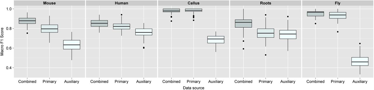
The median macro-F1 scores for the mouse, human, callus, roots and fly datasets were 0.879, 0.853, 0.863, 0.979, 0.965, respectively, for the combined k-NN transfer learning approach. A two sample t-test showed that over 100 test partitions, the mean estimated generalisation performance for the k-NN transfer learning approach was significantly higher than on profiles trained solely from only primary or auxiliary alone for the mouse (p = 2.283e⁻²¹ for primary alone and p = 6.926e⁻⁷⁸ for auxiliary alone), human (p = 1.119e⁻⁷ for primary alone and p = 8.104e⁻³² for auxiliary alone), callus roots (p = 3.761e⁻¹⁷ and p = 3.807e⁻²²), and fly (p = 2.618e⁻⁵ for primary alone, p = 1.379e⁻¹¹² for auxiliary alone) data (Figure 1).

Figure 1:

Boxplots, displaying the estimated generalisation performance over 100 test partitions for the k-NN transfer learning algorithm applied with (i) optimised class-specific weights (combined), (ii) only primary data and (iii) only auxiliary data, for each dataset.

We found that the callus datatset on the full Arabidopsis thaliana proteome did not significantly benefit (neither fall detriment) to the incorporation of auxiliary data. This was unsurprising as this dataset is extremely well-resolved in LOPIT (Supporting Figure 1, top right) and the median macro F1-score over 100 rounds of training and testing with a baseline k-NN classifier resulted in a median macro F1-score of 0.985 (the combined approach yielded a macro F1-score of 0.973).

The k-NN transfer learning classifier uses optimised class weights to control the proportion of primary to auxiliary neighbours to use in classification. One advantage of this approach is the ability for the user to set class weights manually, allowing complete control over the amount of auxiliary data to incorporate. As previously described, the class weights can be set through prior optimisation on the labelled training data. Figure 2 shows the detailed results for the mouse dataset and the distribution of the 100 best weights selected over 100 rounds of optimisation are shown on the top left. We found the distribution of weights in each dataset reflected closely the sub-cellular resolution in each experiment. For example, in the E14TG2a mouse experiments the distribution of best weights identified for the endo-plasmic reticulum (ER), mitochondria and chromatin niches are heavily skewed towards 1 indicating that the proportion of neighbours to use in classification should be predominantly primary. Note, as described in section 2.2.2 if the class weight is assigned to 1, then strictly only neighbours in primary data are used in classification and similarly, if the class weight is 0 then all weight is given to the auxiliary data. If the weight falls between these two limits the neighbours in both the primary and auxiliary data sources is considered. From examining the principal components analysis plot (PCA) (Figure 2, top right) we indeed found that these organelles are well separated in the LOPIT experiment. Conversely, we found that the 40S ribosome overlaps somewhat with the nucleolus cluster (Figure 2, top right) which is reflected in the best choice of class weights for these two niches; they are both assigned best weights of 1/3 and their distribution of best weights is skewed towards 0 indicating that more auxiliary data should be used to classify these sub-cellular classes. If we further examine the class-F1 scores for these two sub-cellular niches (Figure 2, bottom) we indeed find that including the auxiliary data in classification yields a significant improvement in generalisation accuracy (p = 1.122e −16 for 40S ribosome (red) and p = 1.258e⁻¹⁰, nucleolus (pink)). We also found this to be the case for the proteasome, which is overlapping with the cytosol. We found LOPIT alone did not distinguish between these two sub-cellular niches in this particular experiment, however, the addition of auxiliary data from the Gene Ontology resulted in a significant increase in classifier prediction (p = 2.108e⁻¹⁶) as shown by the class-specific box plot in Figure 2, bottom (black). In this framework we are able to resolve different niches in the data according to different data sources, as highlighted in the class-specific box-plots in Supporting Figures 1 to 4.

Figure 2:

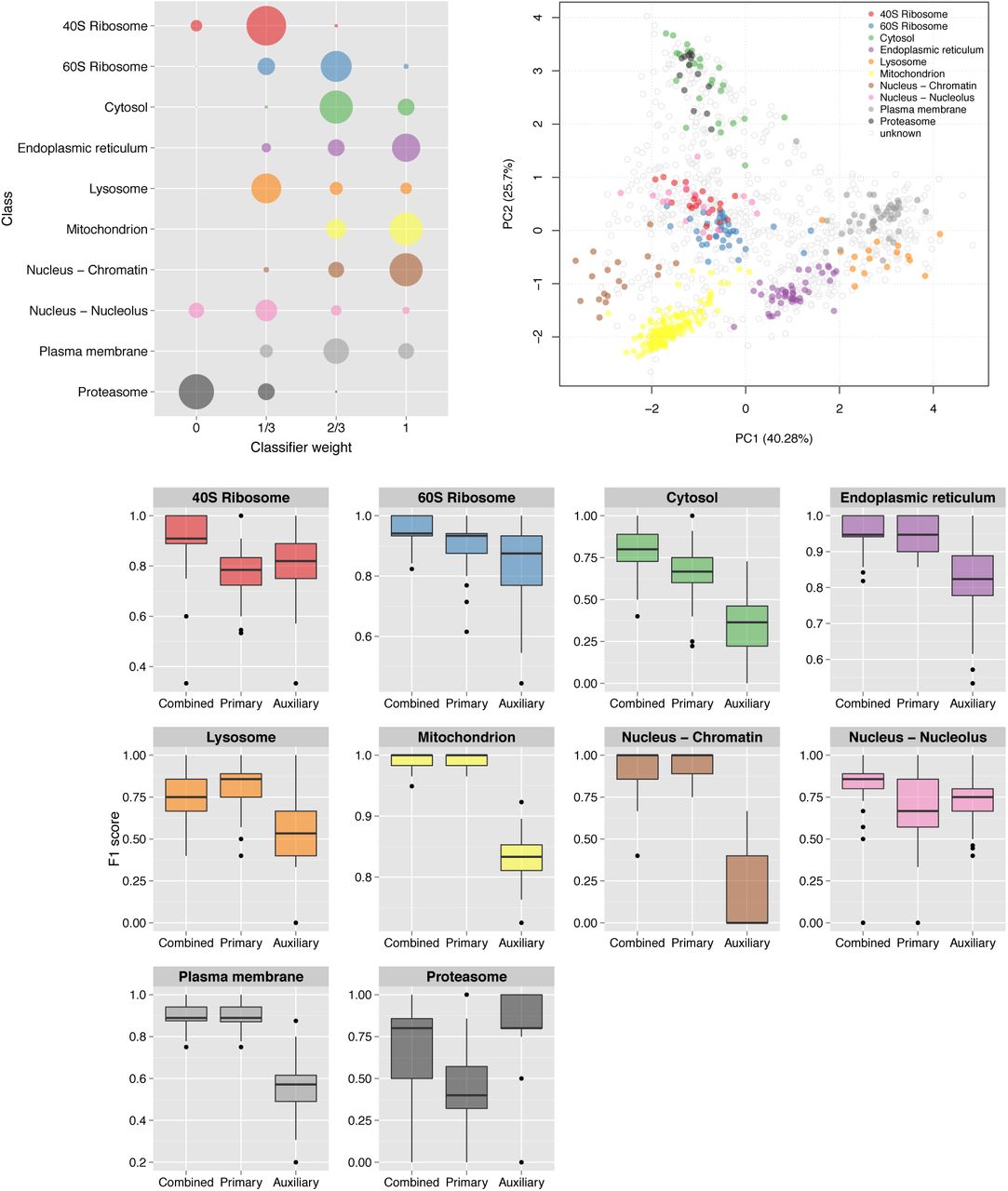
Top left: Bubble plot, displaying the distribution of the optimised class weights over the 100 test partitions for the transfer learning algorithm applied to the mouse dataset. Top right: Principal components analysis plot (first and second components, of the possible eight) of the mouse dataset, showing the clustering of proteins according to their density gradient distributions. Bottom: Sub-cellular class-specific box plots, displaying the estimated generalisation performance over 100 test partitions for the transfer learning algorithm applied with (i) optimised class-specific weights (combined), (ii) only primary data and (iii) only auxiliary data, for each sub-cellular class.

Many experiments are specifically targeted towards resolving a particular organelle of interest (e.g. the TGN in the roots dataset) which requires careful optimisation of the LOPIT gradient. In such a setup sub-cellular niches other than the one of interest may not be well-resolved which may simply be due to the fact that the gradient was not optimised for maximal separation of all sub-cellular niches, but only one or a few particular organelles. Such experiments in particular may benefit from the incorporation of auxiliary data. We found that for the roots dataset all sub-cellular classes, except the TGN sub-compartment, benefitted from including auxiliary data (Supporting Figure 3, bottom), highlighting the advantage of using more than one source of information for sub-cellular protein classification. The best weight for the TGN was found to be 1 (Supporting Figure 3, top left), as expected and indicating high resolution in LOPIT for this class.

Figure 3:

Boxplots, displaying the estimated generalisation performance over 100 test partitions for the SVM transfer learning algorithm applied with (i) optimised class-specific weights (combined), (ii) only primary data and (iii) only auxiliary data, for each dataset.

3.1.2 The SVM transfer learning classifier

Adapting Wu and Dietterich’s classic application of transfer learning [6] we have implemented a SVM transfer learning classifier that allows the incorporation of a second auxiliary data source to improve upon the classification of experimental and condition-specific sub-cellular localisation predictions. The method employs the use of two separate kernels, one for each data source. As described in section 2.2.4 to assess generalisation accuracy of our classifier we employed the classic machine learning schema of partitioning our labelled data in to training and testing sets, and used the testing sets to assess the strength of our classifiers. This was repeated on 100 independent partitions for the (i) SVM TL method, (ii) a standard SVM trained on LOPIT alone, and (iii) a standard SVM trained on GO CC alone.

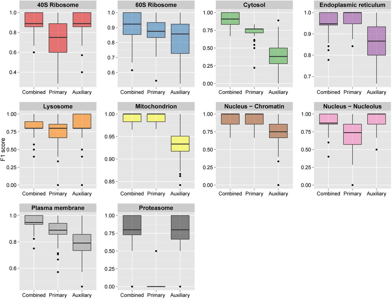
For the SVM TL experiments the resultant median macro-F1 scores for the mouse, human, callus, roots and fly datasets were 0.902, 0.868, 0.956, 0.875, 0.961, respectively, over the 100 partitions. As per the k-NN TL, we found the macro-F1 scores for the SVM TL (Figure 3) was significantly higher than on profiles trained solely from only primary or auxiliary alone; mouse (p = 4.474e⁻⁵⁶ for primary alone and p = 6.313e⁻³⁷ for auxiliary alone), human (p = 7.325e⁻³ for primary alone and p = 1.071e⁻²¹ for auxiliary alone), callus (p = 0.004 for primary alone and p = 1.297e⁻⁹² for auxiliary alone), roots (p = 1.725e⁻⁴⁵ for primary alone and p = 7.846e⁻²⁵ for auxiliary alone), and fly (p = 2.775e⁻³ for primary alone and p = 4.325e⁻¹⁰⁵ for auxiliary alone) data. This was also evident on the organellar level as seen in Figure 4 and Supporting Figures 5 - 8.

Figure 4:

Boxplots, displaying the estimated generalisation performance over 100 test partitions for the SVM transfer learning algorithm applied with (i) optimised class-specific weights (combined), (ii) only primary data and (iii) only auxiliary data, for the mouse dataset.

Figure 5:

Boxplots displaying the distribution of scores assigned to the unknown proteins in the mouse dataset for the k-NN, k-NN transfer learning (TL) algorithm, a Support Vector Machine (SVM) and the SVM TL classifiers. For each classifier the proteins have been split between those that have been classified as incorrect or correct according to known protein localisations found by a recent high resolution map of the mouse proteome.

3.2 Other auxiliary data sources

One of the advantages of the transfer learning framework is the flexibility to use different types of information for both the primary and auxiliary data source. We demonstrate the flexibility of this framework by testing other complementary sources of information as an auxiliary data source.

3.2.1 The Human Protein Atlas

The sub-cellular Human Protein Atlas [66] provides protein expression patterns on a sub-cellular level using immunofluorescently staining for human U-2 OS cells. As described in 2.1.2 we used the hpar Bioconductor package [67] to query the sub-cellular Human Protein Atlas [66] (version 13, released on 11/06/2014). This auxiliary data, to be integrated with our human LOPIT experiment, was encoded as a binary matrix describing the localisation of 670 proteins in 18 sub-cellular localisations supportively identified. Information for 192 of the 381 labelled marker proteins were available. These 192 proteins covered 8 of the 10 known localisations in the human LOPIT experiment and were used to estimate the classifier generalisation accuracy of the (i) the transfer learning approach with both data sources, (ii) the LOPIT data alone and (iii) the HPA data alone, as described previously. As detailed in the supplementary information (Supporting Figure 9), we observed a statistically significant improvement of our overall classification accuracy as well as several organelle-specific results.

3.2.2 YLoc sequence and annotation features

Sequence and annotation features, as described in Table 1, that were used as input from the computational classifier YLoc [61, 62] were selected as an auxiliary data source to complement the LOPIT E14TG2a mouse stem cell dataset. 34 sequence and annotation features were selected using a correlation feature selection, as described in section 2.1.2. Using the LOPIT mouse dataset as our primary data, and the 34 YLoc features as our auxiliary we employed the standard protocol for testing classifier performance (1) using the k-NN transfer learning with both data sources, (2) the primary data alone and (3) the auxiliary data alone, as detailed in section 2.2.4. Although we did not observe a statistically significant improvement using the auxiliary data in the transfer learning framework, we did not see any statistically significant disadvantage in combining information (Supporting Figure 10). Thus we found that incorporating data from auxiliary sources in this framework does not dilute any strong signals in the original experiment, demonstrating the flexibility of the classifier.

3.3 Biological application

We applied the two transfer learning classifiers to a real life scenario to (i) demonstrate algorithm usage, and (ii) highlight the applicability of the method for predicting protein localisation in MS-based spatial proteomics data over other single source classifiers. We used the E14TG2a mouse dataset as our use case. The dataset contained density gradient profiles for 1109 proteins, across 8 fractions, of which 387 proteins were labelled (i.e. identified as known protein markers) distributed among 10 sub-cellular niches (the plasma membrane, endoplasmic reticulum, mitochondria, nucleolus, chromatin, 40S and 60S ribosomal subunits, proteasome, lysosome and cytosol, see supporting table 1), the remaining 722 proteins were unlabelled. We extracted the GO CC auxiliary data matrix for all proteins in the dataset (as described in 2.1.2) and then applied the following four classifiers (1) k-NN (with LOPIT data only), (2) k-NN TL (with LOPIT and GO CC data), (3) SVM (with LOPIT data only) and (4) SVM TL (with LOPIT and GO CC data) for the prediction of the sub-cellular localisation of the unlabelled proteins in the dataset.

As previously discussed, before applying any machine learning classifier one is required to optimise any free algorithmic parameters on the training data as it is widely known that wrongly set parameters can have adverse effects on the classification performance and success of the learner. Following the standard protocol (as described in section 2.2.4) parameter optimisation was conducted on the labelled training data using 100 rounds of stratified 80/20 partitioning, in conjunction with 5-fold cross-validation in order to estimate the free parameters via a grid search, as implemented in the pRoloc package [64]. The best parameters were found to be k = 5 for the k-NN classifier and for the k-NN TL classifier k_P = 5, k_A = 5 and the best class weights were found for the 40S ribosome, 60S ribosome, cytosol, endoplasmic reticulum, lysosome, mitochondria, nucleus - chromatin, nucleolus, plasma membrane and proteasome, respectively. For the SVM classifier we found the best cost to be C = 16 and γ = 10. For the SVM TL classifier we found C = 16, γ_P = 1, γ_A = 0.1. Using these parameters with their associated algorithms we classified the 722 unlabelled proteins in the dataset and obtained a classifier score for each protein.

In supervised machine learning the instances which one wishes to classify can only be associated to the classes that were used in training. Thus, it is common when applying a supervised classification algorithm, wherein the whole class diversity is not present in the training data, to set a specific score cutoff on which to define new assignments, below which classifications are set to unknown/unassigned. The pRoloc tutorial, which is found in the set of accompanying vignettes in the pRoloc package [64], describes this procedure and how to implement this in real practice. Deciding on a threshold is not trivial as classifier scores are heavily dependent upon the classifier used and different sub-cellular niches can exhibit different score distributions.

To validate our results and calculate classification thresholds based on a 5% false discovery rate (FDR) for each of the four classifiers (i.e. k-NN, k-NN TL, SVM, SVM TL) we compared the predicted localisations with the localisation of the same proteins found in the highest resolution spatial map of mouse pluripotent embryonic stem cells to date² [81]. This high resolution map was generated using hyperplexed LOPIT, a novel technique for robust classification of protein localisation across the whole cell. The method uses an elaborate sub-cellular fractionation scheme, enabled by the use of TMT 10-plex and application of a novel MS data acquisition technique termed synchronous precursor selection MS3 (SPS)-MS³ [82], for high accuracy and precision of TMT quantification. The study used state-of-the-art data analysis techniques [65, 64] combined with stringent manual curation of the data to provide a robust map of the mouse pluripotent embryonic stem cell proteome. The authors also provide a web interface to the data for exploration by the community through a dedicated online R shiny [83] application³. From examining the overlap between our new classifications and the localisations in the high resolution mouse map we found 183 of our 722 unlabelled proteins matched a high confidence localisation in the new dataset. Of the remaining, 347 of our proteins were labelled as unknown in the mouse map (i.e. were assigned a low confidence localisation in the experiment), and 192 proteins did not appear in the map. We used the localisation of these 183 high confidence proteins as our gold standard on which to validate our findings and set a false discovery rate for our predictions.

Figure 5 shows the score distributions for correct and incorrect assignments of the unas-signed proteins in the dataset (as validated through the high resolution mouse pluripotent embryonic stem cell map) and the distribution of the scores per classifier. Note, the scores in Figure 5 are not a reflection of the classification power and the score distributions between the four different methods are not comparable to one another as they are calculated using different techniques, as detailed in section 2.2. For both of the single source k-NN and SVM classifiers there is a large overlap in the distribution of scores for correct and incorrect assignments (Figure 5). It is desirable to have a distribution of scores that enables one to choose a cutoff that minimises the false discovery rate. What is evident from examining the score distributions of incorrect and correct assignments in Figure 5 is that by using transfer learning we have increased the discrimination power of the classifier and thus lowered our FDR.

Using our knowledge of the correct/incorrect outcomes of these 183 previously unlabelled proteins we calculated an appropriate threshold on which to classify all unlabelled proteins. Using a FDR of 5% we found assignment thresholds for the SVM (0.85), SVM TL (0.785) and k-NN TL (0.805) to classify the remaining unlabelled proteins. A FDR of 5% was not possible with the k-NN classifier and the lowest achievable FDR was 15% which occurred using the strictest threshold of 1 i.e. only when all 5 nearest neighbours agreed. Comparing the classifications made from the single source classifiers to those made with the transfer learning methods, we found in both cases we get many more assignments using the combined transfer learning approaches compared to the single source methods using a fixed FDR of 5%, as discussed below.

Figure 6 shows the SVM and SVM TL scores assigned to each of the 183 validated proteins. The sub-cellular class is highlighted by solid colours and an un-filled point on the plot represents the case where the two classifiers disagreed on the sub-cellular localisation. We found that the SVM TL classifier gave 70% more high confidence classifications with the same 5% FDR threshold than the single source SVM trained on primary data alone. All proteins that were assigned to a sub-cellular niche with a high confidence score in both the SVM and SVM TL (Figure 6, top right grid) were assigned to the same class. We also found that many proteins outside of the high confidence threshold were assigned the same sub-cellular class using both methods, as indicated by the abundance of solid points on the plot. Of the total 722 previously unlabelled proteins we assigned high confidence localisations for 204 proteins using the SVM TL, and 176 proteins using the k-NN TL method, based on a FDR of 5% (Supporting Tables 7 and 8).

Figure 6:

Scatterplot displaying the scores for the SVM and SVM TL classifiers for the 183 proteins validated by the hyperLOPIT mouse map [81]. Each point represents one protein and its associated classifier scores. Filled circles highlight proteins that were assigned the same sub-cellular class with each classifier, empty circles represent the instance when the two classifiers gave different results. The solid lines show the classification boundaries for the two classifiers at a 5% FDR, above which proteins are classified to the highlighted class, below these boundaries proteins are deemed low confidence and thus left unassigned.

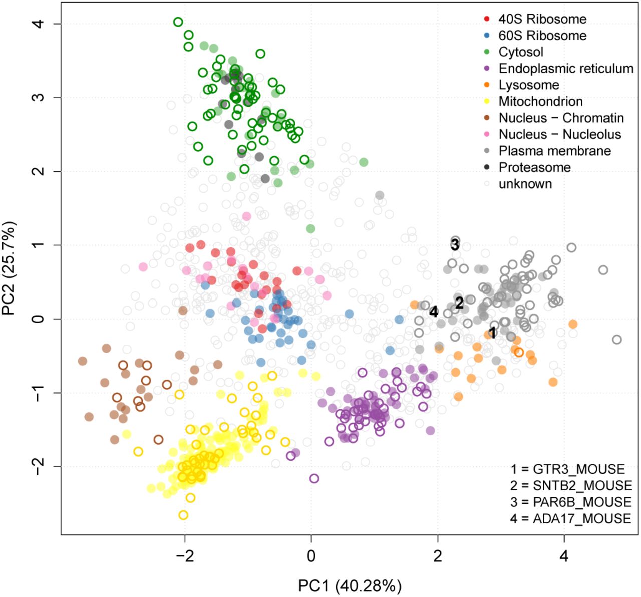
By way of biological validation we investigated additional proteins gained using the SVM TL method (Figure 6, bottom right grid) as novel assignments to one of these classes, the plasma membrane, by searching through the literature for supporting empirical evidence. For example, using the SVM TL method we found four proteins assigned only to the plasma membrane with the SVM TL method (Figure 7) that were also assigned to the plasma membrane in the recent high resolution mouse map (GTR3 MOUSE, SNTB2 MOUSE, PAR6B MOUSE and ADA17 MOUSE). Dehydroascorbic acid transporter (GTR3 MOUSE) is a multi-pass membrane protein which has been previously shown to be a plasma membrane protein in studies isolating the cell surface glycoprotein in Jurkat cells [84]. Beta-2 syntrophin or syntrophin 3 (SNTB2 MOUSE) is a phosphoprotein with PDZ domain through which it interacts with ion channels and receptors. There are confounding reports of the sub-cellular location of this peripheral protein. It associates with dystrophins and has no signal sequence. It is found mostly in muscle fibres and brain [85], but to date, its role has not been studied in mouse embryonic stem cells. Given its association with ion channels and receptors, it is perfectly feasible that the steady location of this protein in stem cells is plasma membrane. Partitioning defective 6 homolog beta (PAR6B MOUSE) is a peripheral membrane protein thought to be in complex with E-cadherin, aPKC, and Par3 at the plasma membrane [86], where it functions to guide GTP-bound Rho small GTPases to atypical protein kinase C proteins [87]. Disintegrin and metalloproteinase domain-containing protein 17 (ADA17 MOUSE) is a single pass plasma membrane protein which functions to cleave the intracellular domain of various plasms membrane proteins including notch and TNF-alpha [88]. It is therefore involved in the upstream events in several signalling pathways. It has a 17 amino acid N-terminal signal sequence suggestive of its function as a membrane protein.

Figure 7:

Principal components analysis plot (PCA) of the E14TG2a mouse stem cell dataset. Proteins are clustered according to their density gradient distributions. Each point on the PCA plot represents one protein. Filled circles are the original protein markers used in classification, hollow circles show new locations as assigned by the SVM TL classifier. The 4 proteins GTR3_MOUSE, SNTB2_MOUSE, PAR6B_MOUSE and ADA17_MOUSE that were found in the SVM TL method and not in an SVM classification with LOPIT only are highlighted.

The full list of localisation predictions for all proteins in the mouse E14TG2a dataset can be found in the R data package pRolocdata.

3.4 A Comparison: KNN vs SVM

We compared the macro- and class-F1 scores from all experiments in 3.1 on the 5 datasets used to assess the classifier performance of the k-NN TL and SVM TL methods. We found that no single method systematically outperformed the other, as described further in section 5 of the supporting supplement.

When applying the SVM TL and k-NN TL classifiers to the unlabelled proteins in section 3.3 an analysis of the final assignments (as classified based on FDR of 5%) showed that there was no contradiction in results. The predicted localisations were in high agreement and if not assigned to the same class as the other classifier, proteins were found to labelled as unknown i.e. were low confidence assignments (see Supporting Table 9).

4 Conclusion

In this study we have presented a flexible transfer learning framework for the integration of heterogeneous data sources for robust supervised machine learning classification. We have demonstrated the biological usage of the framework by applying these methods to the task of protein localisation prediction from MS-based experiments. We further show the flexibility of the framework by applying these methods to the five different spatial proteomics datasets, from four different species, in conjunction with three different auxiliary data sources to classify proteins to multiple sub-cellular compartments. We find the two different classifiers; the k-NN TL and SVM TL, perform equally well and importantly both of these methods outperform a single classifier trained on each single data source alone. We further applied the algorithm to a real life use case, to classify a set of previously unknown proteins in a spatial proteomics experiment on mouse embryonic stem cells, which was validated using the most high resolution map of the mouse E14TG2a stem cell proteome to date [81]. We find integrating data from a second data source directly in to classifier training and classifier creation results in the assignment of proteins to organelles with high generalisation accuracy. Finally, we find that using freely available data from repositories we can improve upon the classification of experimental and condition-specific protein-organelle predictions in an organelle specific manner.

To our knowledge, no other method has been developed to date that allows the incorpo-ration of an auxiliary data source for the primary task of predicting sub-cellular localisation in spatial proteomics experiments. In this study we have developed methods that not only allow the inclusion of an auxiliary data source in localisation prediction, but we have created a flexible framework allowing the use of many different types of auxiliary information, and furthermore allows the user complete control over the weighting between data sources and between specific classes. This is extremely important for the analysis of biological data in general, and spatial proteomics data in particular, as many experiments are targeted towards resolving specific biologically relevant aspects (sub-cellular niches in spatial proteomics) and thus users may wish to control the impact of auxiliary information for aspects that have been specially targeted for analysis by the primary experimental method. In this context the setting of weights manually in the k-NN transfer learning classifier allows users complete power to explicitly choose whether to call upon an auxiliary data source or simply use data from their own experiment, on an organelle-by-organelle basis.

The effectiveness of using databases as an auxiliary data source will depend greatly on abundance and quality of annotation available for the species under investigation. For example, human is a well-studied species and there is a large amount of information available in the Gene Ontology and Human Protein Atlas. Furthermore, some organelles are easier to enrich for and thus there exists much more information available to utilise as an auxiliary source on a organelle by organelle basis. The transfer learning methods we present here allow the inclusion of any type of auxiliary data, provided of course there is information available for the proteins under investigation.

The integration of auxiliary data sources is a double-edged sword. On the one hand, it can shed light on (i) the primary classification task by reinforcing weak patterns or (ii) complement the signal in the primary data. On the other hand however it is easy to dilute valuable signals in an expensive experiment by shadowing the uniqueness, and hence biologically relevance of the experimental primary data when integration is not performed with care. Thus one needs to be cautious with data integration in general and not overlook the biological relevance of the primary data. Here, we provide a solution to this issue and demonstrate that under this learning framework, one never can do worse than using primary data alone: the k-NN transfer learning classifier uses optimised class-specific weights so as not to penalise any strong signals in the primary, if no signal is found in the auxiliary, similarly, the SVM transfer learning method uses optimised data-specific gamma parameters for each data-specific kernel.

The transfer learning framework forms part of the open-source open-development Bio-conductor pRoloc suite of computational methods available for organelle proteomics data analysis. Moreover, as the pipeline utilises the formal Bioconductor classes, different data types, for example from gene expression technologies among others, can be easily used in this framework. The integration of different data sources is one of major challenges in the data intensive world of computational biology, and here we offer a flexible and powerful solution to unify data obtained from different but complimentary techniques.

Acknowledgements

LMB was supported by a BBSRC Tools and Resources Development Fund (Award BB/K00137X/1). LG was supported by the European Union 7^th Framework Program (PRIME-XS project, grant agreement number 262067) and a BBSRC Strategic Longer and Larger grant (Award BB/L002817/1). DW and OK acknowledge funding from the European Union (PRIME-XS, GA 262067) Deutsche Forschungsgemeinschaft (KO-2313/6-1). The authors would also like to thank Dr Matthew Trotter from Celgene Institute Translational Research Europe for his insightful comments and Dr. Dureid El-Moghraby from the High Performance Computing Service, University of Cambridge for his support

Footnotes

• Abbreviations LOPIT: Localisation of Organelle Proteins by Isotope Tagging, PCP: Protein Correlation Profiling, ML: Machine learning, TL: Transfer learning, SVM: Support vector machine, PCA: Principal component analysis, GO: Gene Ontology, CC: Cellular compartment, iTRAQ: Isobaric tags for relative and absolute quantitation, TMT: Tandem mass tags, MS: Mass spectrometry

• ¹ Note that it is possible for the linear programme to have no solution, although we found this to be extremely rare. When this was the case the classifier reverted to predicting the most common class in the labelled data.

• ² Currently under review

• ³ https://lgatto.shinyapps.io/christoforou2014