

Abstract
Ash dieback due to Hymenoscyphus fraxineus is threatening the Fraxinus excelsior species in most of its natural range in Europe and it is becoming obvious that other species in the Fraxinus genus are susceptible to the disease. The fungal pathogen apparently originates from Asia where it may act as an endophyte of local species like F. mandshurica. Previous studies reported significant levels of genetic variability for susceptibility in F. excelsior either in field or inoculation experiments. The present study was based on a field experiment planted in 1995, fifteen years before onset of the disease. Crown and collar status were monitored on 788 trees from 23 open-pollinated progenies originating from 3 French provenances. Susceptibility was modelled using a Bayesian approach where spatio-temporal effects were explicitly taken into account, thus providing accurate narrow-sense heritability estimates (h2). While moderate narrow-sense heritability estimates for Crown Dieback (CD, h2 = 0.42 in this study) have already been reported in the literature, this study is first to show that Collar Lesions are also heritable (h2 = 0.49 for prevalence and h2 = 0.42 for severity) and that there is significant genetic correlation between the severities of both traits (rspearman=0.40). Unexpectedly, their spatio-temporal dynamics followed almost opposite patterns. While no significant Provenance effect were detected for any trait, significant Family effects were found for both CD and CL. Moreover, the analysis strategy implemented here allowed to compute Individual Breeding Values (IBV) and to show that there is more genetic variability within families than between families. In agreement with previous reports, early flushing correlates with better crown status. Consequences of these results in terms of management and breeding are discussed.
Introduction
An extensive scientific review on the European ash dieback crisis was published very recently (McKinney et al. 2014), thus allowing for a brief overview here. Severe dieback of European common ash (Fraxinus excelsior) was first reported in Poland and Lithuania in the early 1990s (Lygis et al. 2005; Przybyl 2002). Since then, the pathogen infected at least 26 countries with its current South-Western limit now in Central France. The observed symptoms have long been thought to result from a combination of disease outbreaks (e.g. phytoplasma, mycoplasma, phytophthora, etc.) due to changes in climatic factors and emergence of new pathogens and vectors (Pliura and Baliuckas 2007). It was fourteen years after the first reports that an ascomycete was finally identified as the primary causal agent (Kowalski 2006). Firstly described as a new fungal species (i.e. Chalara fraxinea), it was soon suggested that it could be the anamorphic stage of Hymenoscyphus albidus, a widespread native decomposer of ash litter (Kowalski and Holdenrieder 2009). However, more detailed molecular investigations revealed that the disease agent in fact belongs to a distinct and previously undescribed species now referred to as H. fraxineus (Baral et al. 2014). Several findings pledge for the species being an invasive pathogen in Europe. First, the fungus could not be found in disease-free areas like Western and Central France (Husson et al. 2011) whereas it completely replaced H. albidus in infected areas of Denmark (McKinney et al. 2012b). Second, indications of a founder effect were reported at some loci (Bengtsson et al. 2012). Third, a study revealed that some fungi isolated from the Asian Ash species Fraxinus mandshurica in Japan and initially reported as Lambertella albida in fact belong to H. fraxineus (Zhao et al. 2012).
Knowledge on the life cycle of H. fraxineus increased considerably when Gross et al. (2012) described mating type (MAT) loci and concluded on a heterothallic mating system. Sexual reproduction is mediated through conidia which are produced in autumn on dead ash petioles in the litter and possibly on other dead tissues also. A single petiole can host multiple genotypes which overwinter in the form of black pseudosclerotial plates. Apothecia are formed in summer and they release ascospores that are wind-dispersed and that germinate on ash leaflets or petioles forming an appressorium (Cleary et al. 2013). Once in the leaf tissue, the mycelium develops intracellularly, moving through the cells and easily colonizing the phloem, paratracheal parenchyma and parenchymatic rays (Dal Maso et al. 2012). Schumacher (2011) proposed an invasion model where the fungus invades the pith and vessels preferentially via the ray parenchyma, where growth is fastest, and subsequently spreads outward towards the cambium and phloem, triggering the colonization of the necrotic bark by secondary fungi. Symptoms of the disease are many: wilting of leaves, necrotic lesions on leaves, necrosis on twigs, stems and branches, and collar lesions. Collar lesions have been described quite late (Lygis et al. 2005) and there is still some controversy about these lesions being induced by H. fraxineus or by other fungi like Armillaria sp. or Phytophthora sp. (Bakys et al. 2011; Enderle et al. 2013; Husson et al. 2011; Orlikowski et al. 2011; Skovsgaard et al. 2010).
With a natural range that stretches from Iran to Ireland and from Southern Scandinavia to Northern Spain (Dobrowolska et al. 2011), F. excelsior is the most common and the most northern of the 3 Fraxinus species native to Europe, and thus the first one to face this new threat. Less is known about field reaction of F. angustifolia and F. ornus to the disease although some inoculation tests tend to indicate that F. ornus, which belongs to a distinct section, is much more resistant that the other two species (Kirisits et al. 2010; Kräutler and Kirisits 2012). Detailed quantifications are scarce, but consequences of the disease can be severe. In Lithuania, 10 years after the first report, over 30,000 ha of common ash stands were reported to be affected and mortality was estimated to be 60% state wide while in some parts of the country only about 2% of the trees remained visually healthy (Juodvalkis and Vasiliauskas 2002). In 2006, ash dieback was still present on 9,400 ha despite extensive clear cuts of severely damaged stands (Pliura and Baliuckas 2007). In Southern Sweden, one fourth of all ash trees were reported as dead or severely damaged 7 years after the first report (Fischer et al. 2010). In some parts of North-Eastern France, only 3% of the trees remained completely healthy 2 years after the first reports (Husson et al. 2012). These figures corroborate the findings from McKinney et al. (2011) on 39 clones from 14 Danish populations where only one clone out of 39 maintained an average damage level below 10% in two replicated field trials. The computed broad-sense heritability estimates (i.e. 0.40–0.49 in 2009, six years after the first report in Denmark) were however indicative of a strong genetic control, meaning that there is an adaptive potential and that breeding material with low susceptibility would be possible. Same conclusions were drawn from another study where 106 clones from 27 Swedish stands were evaluated (Stener 2013). No significant Stand (i.e. Provenance) effect was found in any of these two studies. When comparing 320 open-pollinated maternal progenies from 24 European provenances (8 countries) in two field trials in Lithuania, Pliura et al. (Pliura et al. 2011) found significant Provenance and Family effects, with the best provenances being local ones. Narrow-sense heritability of health condition at the age of four (respectively eight) years varied between 0.60 and 0.92 (respectively 0.40 and 0.49). The same authors recently published results from a pluriannual multi-site clonal evaluation of the best trees (47 clones) and found broad-sense heritabilities of 0.38 to 0.40 for tree health conditions (Pliura et al. 2014). Unfortunately, the number of clones with at least one infected ramet increased from 45.9% to 100% in just one year in this selected material. Kjaer et al. (Kjaer et al. 2012) also found significant Family effects when studying 101 open-pollinated progenies from 14 Danish provenances. They did not detect any Provenance effect and narrow sense heritability estimates for crown damage were in the range 0.37–0.52. A third study based on open-pollinated maternal progenies was published very recently (Lobo et al. 2015). Again, significant differences were observed among families and not among provenances while narrow-sense heritabilities for crown damage ranged from 0.20 to 0.53.
The present study is only fourth to analyze the genetic variability of common ash for resistance/tolerance to H. fraxineus using open-pollinated maternal progenies. It is based on a 20-year old field trial with 23 half-sib families from 3 French provenances. The trial is located in the area where Ash dieback was first detected in France in 2008. Because the stand has been monitored every year since 2010 for disease incidence, spatio-temporal components of disease spread could be taken into account to avoid confounding disease escape and resistance. Moreover, a Bayesian approach was used instead of the classical frequentist analysis. Bayesian methods accommodate complex spatio-temporal structures in a more straightforward way and their results are directly interpretable in terms of posterior probabilities. In addition, they are also more suitable for modelling data which deviates heavily from normality, as it is frequently the case during early stages of disease spread. Moreover, it leverages information from previous knowledge with actual observed data, which can be critical in situations where data are little informative (Mila and Carriquiry 2004). This study is also first to report on the genetic parameters for collar lesions and on the genetic correlation with crown defoliation.
Material and Methods
Experimental design
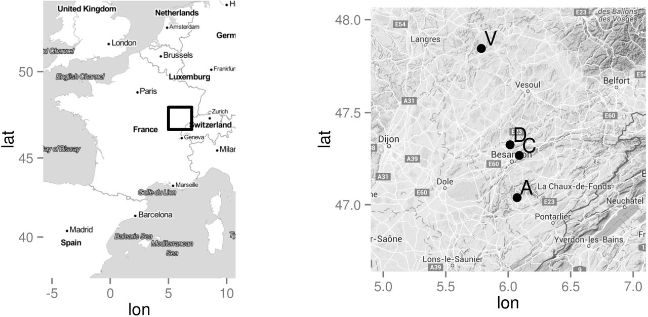
The studied material consisted in 23 open-pollinated F. excelsior maternal progenies from 3 North-Eastern French provenances. Although located less than 40 km apart (Figure 1), these provenances differ for elevation and soil composition and structure. Vernois-sur-Mance is located 200 m high in a river valley. The soil is composed of siliceous deposits with a clay-loam structure turning into a sandy-clay structure with evidences of hydromorphy below 50 cm depth. Chalèze is located on a steep North-West facing slope averaging 300 m high on a calcareous colluvial brown soil with a clay-loam structure on marly limestone bedrock. Amancey is located on a 620 m high plateau composed of a sometimes superficial clay-loam soil on a hard lime-stone bedrock. Mother trees were selected at random within each provenance. Seeds were collected in 1992, cold-stratified, germinated and raised in nursery until plantation in January 1995.

Provenance (A=Amancey, C=Chalèze, V=Vernois-sur-Amance) and study site (D=Devecey) locations.
The trial was established in Devecey, 61 km from the furthest provenance, on a winter tilled agricultural land located 250 m high. Planting was done at a spacing of 4 m × 4 m following a randomized incomplete block design. Depending on plant availability, each family was represented in two to ten blocks plus the border except two families that were represented in the border only. Each block contained 16 families, each represented by 4 trees that were distributed among 4 sub-blocks. Each family was thus represented by 8 to 68 trees in the whole trial including the border (Table 1).
Studied F. excelsior material
Measurements
A first investigation for presence of H. fraxineus was conducted in February 2009 and did not reveal any symptom. The first signs of infection were observed in February 2010 and presence of the fungus was confirmed by real time PCR (French Department of Agriculture, personal communication). Crown dieback (CD) was measured in July 2010, July 2011, June 2012, June 2013 and June 2014 using a 0 to 5 ranking scale according to the proportion of dead branches: 0 - no dead branches; 1 - less than 10% dead branches; 2 - 10 to 50% dead branches; 3 - 50 to 80% dead branches; 4 - more than 80% dead branches; 5 - dead tree. For data analysis, classes were subsequently converted to their median value (i.e. 0, 0.05, 0.30, 0.65, 0.90 and 1). Collar lesions (CL) were measured in July 2012 and June 2013. Detecting and measuring them required scratching the bark using a triangular scraper, this is why this measurement was conducted for 2 years only. As several lesions can occur on the same tree, basal width of all lesions were cumulated and divided by the basal girth (BG) of the tree to compute CL as a 0 to 1 girdling index (Figure fig:photo). Bud flushing was measured once, three years after planting, using a 1 (late) – 5 (early) ranking scale.
Data analysis
We analyzed each symptom independently using a sequence of statistical models of increasing complexity and flexibility. All of the fitted models for CD belong to the family of Linear Mixed Models (LMM). This is, the vector y of n measurements of phenotypic values are described as a linear model with a vector of p fixed effects (β) and a vector of q random effects (u). In matrix form,
 where X and Z are n×p and n×q incidence matrices, respectively, and ε is the vector of residuals. Furthermore, both u and ε are assumed to be independent from each other and to follow a zero-mean Gaussian distribution with covariance matrices
  and σ2I respectively, where R is a q × q structure matrix, and I is the n × n identity matrix.
Note that there can be several independent random effects with specific variances and structure matrices. However, they can be stacked in a single vector u with a block-diagonal covariance matrix where each block is the covariance matrix for the corresponding component. Similarly, the incidence matrix Z binds the individual incidence matrices side-by-side in the correct order.
The normality of the residuals is a delicate assumption to make for response variables that are categorical (CD) or restricted to the interval 0–1 (CL). However, it is very convenient from a computational point of view, and this approximation is commonly found in other studies (Kjaer et al. 2012; Pliura et al. 2011). We performed a transformation of the CD variable to improve the adjustment to this hypothesis. Specifically, we worked with


Collar lesions (CL) were cumulated and expressed as a girdling index (i.e. L1 + L2 + … + Ln over the basal circumference of the tree).
The CL variable did not admit any reasonable normalizing transformation, due in part to a large proportion of zeros, and also to a heavily skewed distribution of the positive observations. In consequence, we used a mixture of Generalized Linear Mixed Models (GLMM) for this trait. A GLMM is an extension of a LMM for non-Gaussian data. The observations are assumed to be an independent random sample from some distribution of the exponential family conditional to the mean, which is modelled as a non-linear function of the linear predictor:
 where g is an appropriate link function, μ is the mean, and θ is a vector of additional distribution-specific parameters.
Model inference and comparison
All analyses were performed using R (R Core Team 2015). The models were fitted from a Bayesian perspective using the Integrated Nested Laplace Approximation (INLA) methodology (Rue and Martino 2009) and software (Rue et al. 2014). We used the Marginal Likelihood, the DIC (Spiegelhalter et al. 2002) and the WAIC (Watanabe 2010) as model selection criteria. The Marginal Likelihood is scaled by a factor of −2 (also known as the Deviance), so that for all three criteria, lower values are better.
Model M1 (Table 2) was also fitted using REML (Bates et al. 2015), to compare results with previous literature using the same methodology. We checked that Bayesian and frequentist point estimates of the variance components were similar and thus we report only the Bayesian results.
Model comparison for TCD. The variables in the Linear Predictor are the year, the block, the family (Fam), the family by block interaction, the individual breeding value (IBV), the spatio-temporal effect (ST), the provenance (Prov) and the bud flush precocity (BF).
Statistical models for Crown Dieback
Table 2 summarizes the components of the linear predictor for all the competing models of TCD.
Model M1 was used as a reference model as it uses only unstructured random effects, which is the most basic setting. Among all tested models, this one is the most similar to what was commonly used in previous studies on the genetic diversity of resistance to H. fraxineus (Kjaer et al. 2012; Pliura et al. 2011).In other words, the matrix R is an identity matrix for all random effects. It includes fixed Year and Block effects and unstructured random Family and Family x Block effects. Initially, we also included fixed Provenance and Provenance x Block effects but the Provenance effect was not significant and a Likelihood Ratio Test confirmed that this model was not significantly better than M1 (χ2 (22) = 31.176, p = 0.093).
In model M2, the unstructured random Family effect was replaced with an additive-genetic individual effect (i.e. a vector of Individual Breeding Values, IBV). This is a structured random effect with a known covariance structure given by the family kinship. Specifically, the covariance matrix is
 where
where  is the unknown additive genetic variance in the base population and where the additive-genetic structure matrix A has elements Aij = 2Θij, i.e., twice the coefficient of coancestry between the individuals i and j (see for example, (Lynch and Walsh 1998). The Family x Block interaction effect was also removed since its effect was completely absorbed by the individual genetic effect.
Model M3 replaced the unstructured block effect by a Spatio-Temporal random effect (ST). ST was modelled based on a Gaussian spatial process evolving in time, thus allowing for continuous environmental variation. Evaluated in the spatiotemporal locations of the observations, the values of the Gaussian process follow a Normal distribution with a covariance structure given by the distance, in space and time, between observations. Specifically, the spatio-temporal structure is built as the Kronecker product of separate temporal and spatial processes. The temporal process is simply determined by an autocorrelation parameter ρt between observations, while the spatial process is defined by a Matérn covariance function with parameters of shape (a.k.a. smoothness) ν, spatial scale κ and precision τ2. The smoothness parameter is fixed to ν = 1 for convenience. The spatial scale parameter is associated with the effective range of the spatial process, so that the correlation between locations at a distance  is approximately 0.13. Finally, the marginal variance of the spatial process is given by
  . This yields a structured random effect with a parametric covariance matrix as follows:

Consequently, while the global temporal trend is captured by the explicit Year effect in this model, the ST structure accounts for heterogeneous spatial deviations from the main trend both in space and time.
Models M4 and M5 included, in addition, two potentially explanatory variables. Namely, the provenance and the bud-flush precocity, which entered as fixed effects, respectively.
Finally, two variations of M5 were fitted in order to answer specific scientific questions. Model M5.1 is a re-parameterization introducing an explicit Family effect allowing to split the genetic variance into the inter-family and intra-family components and to compare their relative magnitudes. Computationally, this requires introducing sum-to-zero constraints for each family in the additive-genetic effect for preserving the identifiability of the model. Lastly, Model M5.2 forces the explicit Family effect to be null. Comparing this model with M5 allows testing the hypothesis of significant differences in mean genetic values between families.
Statistical models for Collar Lesions
We considered this variable as the result of two different processes or stages. First, there is the process determining whether a tree becomes infected or not. Second, for those trees that are actually infected, there is the process determining how severely it is affected by the disease. Different factors could potentially affect the two processes in different ways. This includes the genetics and the microenvironment.
Therefore, we analyzed the two processes separately. The pattern of zeros (i.e. inversely related with the disease prevalence) was modelled with a Bernoulli likelihood while the strictly positive observations (i.e. disease severity) were assumed to follow a continuous distribution with positive support.
We considered Beta and Gamma as candidate distributions for the continuous component, and performed a preliminary assessment to determine which one fitted the data better. This consisted of fitting models M0.1 and M0.2 (see Table 4) including all the potentially explanatory fixed effects.
For the rest of the models, we systematically used an individual additive-genetic effect and a spatio-temporal effect as defined in the previous subsection. We then performed a variable selection procedure separately for the binary and continuous components (Tables 3 and 4, respectively), using the Gamma likelihood for the latter. To check the relevance of the basal circumference (BC) as an explanatory variable, we used different parameterizations of this factor. First (M1.1), we split the variable into 6 categories (see Figure 5); in M1.2 we considered also the interaction with the Year; in M1.3 and M1.4 we used the variable as a linear and quadratic regressor respectively; finally, in M1.5 we considered a non-parametric random function of the variable using a second-order random walk. We also considered the provenance (PROV) using only its main effect (M2.1) and also its interaction with the Year (M2.2).
Model comparison for the binary component of CL. The variables in the Linear predictor are the year, the spatio-temporal effect (ST), the individual breeding value (IBV), the Basal Circumference (BC) and the provenance (PROV).
Model comparison for the continuous component of CL. The variables in the Linear predictor are the family (FAM), the provenance (PROV), the year, the Basal Circumference (BC), the spatio-temporal effect (ST) and the individual breeding value (IBV).
For the final model, we integrated both components into a mixture of two GLMMs.
For a measurement yijk taken in year i, at the location j for the individual k, we assumed that

We specified a hierarchical model for the parameters pijk, aijk and bijk using appropriate link functions of the expected values of the respective distributions. Specifically, calling μ = E [y|y > 0] = a/b, we defined two linear predictors

For each linear predictor, Yeari is the fixed effect of the year i = 2012, 2013; sij is a structured Spatio-Temporal (ST) random effect and ak is a structured additive-genetic random effect at individual level (i.e. a vector of Individual Breeding Values, IBV). The ST structure was built as the Kronecker product of separate temporal and spatial zero-mean Gaussian processes, as in Eq. 2. Finally, the structured additive-genetic effect followed a zero-mean multivariate Normal distribution with a known covariance structure given by the family kinship, as in Eq. 1.
Prior distributions
All the fixed effects had a vague zero-mean Gaussian prior with variance of 1,000.
For the variance  of the additive-genetic effect we used an inverse-Gamma with shape and scale parameters of 0.5. This is equivalent to an Inverse-chi-square with 1 df, and places the 80% of the density mass between 0.05 and 15, with a preference for lower values.
For the ST structure, the priors were set independently for the spatial and temporal structures. INLA provides a bivariate Gaussian prior for the logarithm of the positive parameters κ and τ2 of the spatial Matérn field. Its mean and variance were chosen to match reasonable prior judgements about the range and the variance of the spatial field. Specifically, the spatial range had to be between 5 and 38 tree spacings, the latter being the length of the shortest side of the field. There might well exist very short-ranged environmental factors affecting one or two trees at a time, but the model would not be able to separate them from random noise. On the other extreme, there certainly are environmental factors with a larger range than the field diameter, but again, this would be virtually indistinguishable from the global mean of the field. Moreover, the results were found to be very robust to small variations of these prior statements.
Heritability estimates
All heritability estimates have been computed by Monte Carlo simulation given the posterior distributions of the relevant variance parameters. Specifically, we sampled 5,000 independent observations of each variance from their posterior distribution, and derived a posterior density for the heritability.
In general, the narrow-sense heritability is computed as the ratio between the additive-genetic variance and the phenotypic variance. However, this can be implemented in practice in different ways, depending on the specific model and the researcher goals and criteria.
For CD, since there was no direct estimate of the additive-genetic variance of the base population in model M1, it was indirectly estimated using the relationship
 where
where  is the variance between families (Lynch and Walsh 1998). This assumes that the individuals within a family are half sibs under random mating, free recombination and gametic phase equilibrium. The phenotypic variance is simply the sum of the variance components of the model. Namely, the variances of the Family effect, of the Family x Block effect and the residual variance.
Models M2 and M3 provide direct estimates of the additive-genetic variance. In model M2, there is no interaction between Family and Block, therefore the phenotypic variance is reduced to the sum of the additive-genetic variance and the residual variance. In model M3, we included the variance of the ST effect in the phenotypic variance, following accepted guidelines (Visscher et al. 2008). For comparability with models M1 and M2, we also presented the result excluding this term from the denominator.
Estimating the heritability of the CL symptom is more complex. First, because there are two different traits in the model, and thus two different measures of heritability. But more importantly, because both with a Binomial and Gamma likelihoods, the phenotypic variance is a function of the mean, and thus varies from observation to observation. Furthermore, although the additive-genetic variances are assumed common to the population, the phenotypic variance cannot be decomposed additively into genetic and residual components.
Most approaches in the literature dealing with binary data use the so-called Threshold Models, where the data are assumed to be deterministically 0 or 1 depending on whether some unobserved latent Gaussian variable reaches some threshold (see, for example, Dempster and Lerner 1950). In our case the response variable given the latent structure is random rather than deterministic. Therefore, the residual variability comes from the likelihood distribution, which is in a different scale than the genetic variance parameter. However, this is equivalent to a threshold model with an additional residual term following a Logistic distribution. This results in the following formula for the heritability of the binomial component in the latent scale:
 where π2/3 is the variance of a Logistic distribution (Nakagawa and Schielzeth 2010), and
  is the variance of the ST effect. Analogously to CD, we also present the heritability excluding the ST variance from the denominator.
For the continuous component we followed the general simulation-based approach for a GLMM described in de Villemereuil et al. (2015). Unfortunately, this method does not easily allow excluding the ST variance from the denominator, and therefore we only computed the full version of the heritability for this component.
Results
Crown dieback occurrence and severity
From 2010 to 2014, mean CD increased from 0.01 to 0.27 but the distribution of individual values remained highly skewed to the right during the whole study time with most trees showing less than 50% dead branches (i.e. CD < 0.5, Figure 3). In 2010, when disease started to be seen, 53 trees (i.e. 7%) had visible crown dieback including four trees with CD > 0.5. Although one of these four trees died in less than one year, the proportion of dead trees reached only 3% in 2014 while the proportion of trees with CD > 0.5 increased to 19%. The annual decrease in the proportion of trees without visible CD was similar in 2011 and 2012 (−24% and −26%, respectively) but it accelerated in 2013 (−53%) and again in 2014 (−74%), leading to a situation where only 49 trees (i.e. 6%) remained free from CD in 2014. When computing the 3104 values of individual annual increments for CD over the four years of the study, only 73 negative values were found (i.e. 2.3%).

Crown dieback (CD) progress over time.
Collar lesions occurrence and severity
From 2012 to 2013, mean CL increased from 0.05 to 0.14. Collar lesions were found on 29% of the trees in 2012 and this proportion doubled in just one year. Mean CL values computed on symptomatic trees only were 0.19 and 0.23 for 2012 and 2013, respectively. As for CD, the distribution of CL was skewed to the right with only 24 trees with CD > 0.80 in 2013 (Figure 4). Among them, four had their collar totally rotten in 2013 and they were dead the next year. Fifty eight negative values were found for the 2012–2013 increment in CL with only 12 increments below −0.1 (i.e. 1.5 % of all computed increments). These negative increments were most probably artefactual due to the impossibility to measure basal girth and lesion length at exactly the same level each year due to the curved shape of the trunk basis.

Distribution of individual values for collar lesions (CL) expressed as a 0–1 girdling index in 2012 (grey bars) and in 2013 (white bars). Individuals without collar lesions (CL=0) are not shown (i.e. 550 trees in 2012 and 305 trees in 2013).
Although a positive but non-significant trend was observed in 2012, collar lesion occurrence was not clearly related to basal circumference neither in 2012 nor in 2013 (Figure 5). In 2013, only the very few trees with basal circumference below 30 cm had significantly fewer basal cankers.

Occurrence of collar lesions (CL) according to basal circumference categories and Crown Dieback (CD) severity by year. Error bars = 95% confidence intervals for the proportions, considered independently from each other.
Short-distance effect on both symptoms
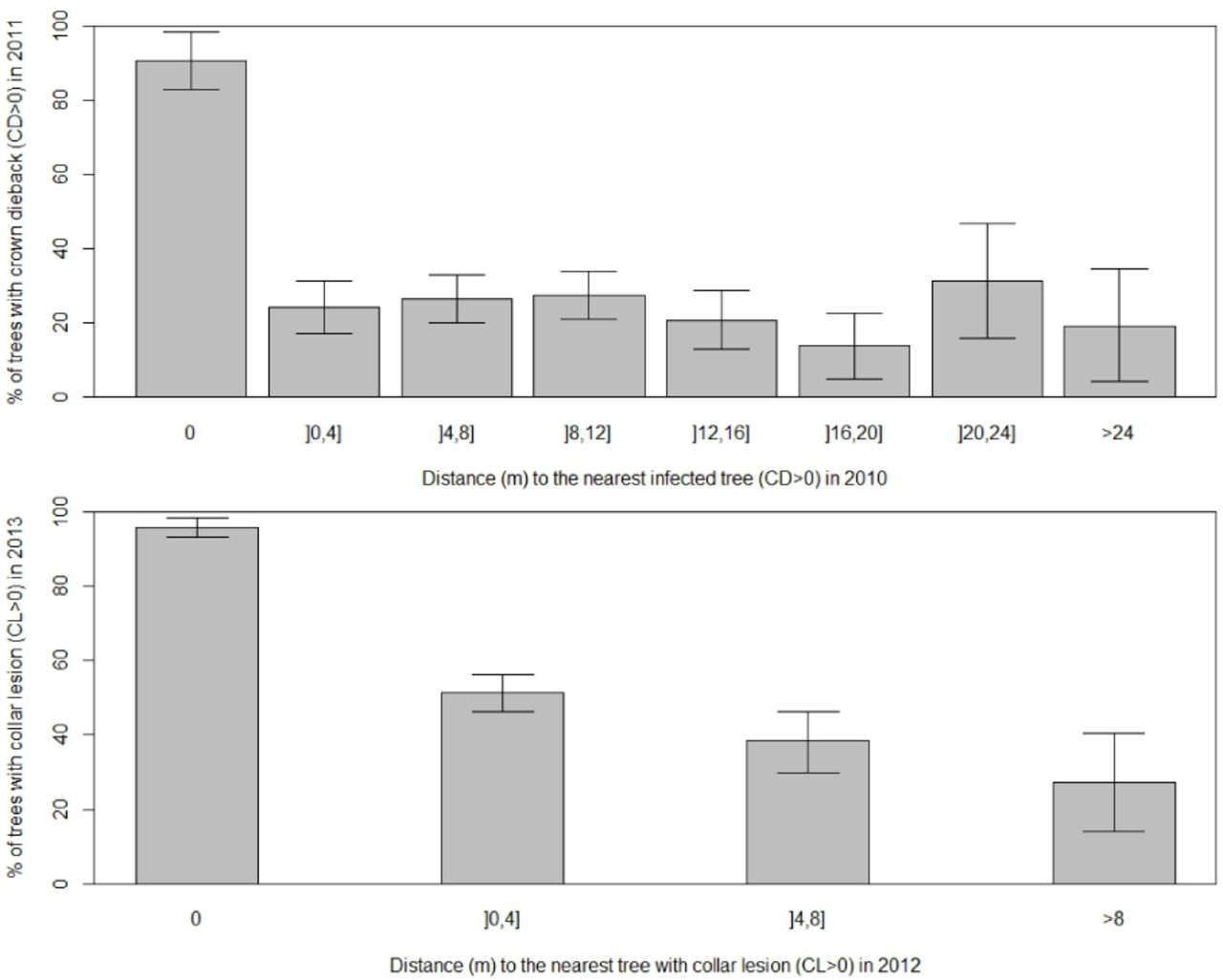
There was no clear evidence of an effect of the distance to the nearest infected tree in 2010 on the occurrence of CD in 2011 (Figure 6). On the other hand, trees located less than 4 m from an infected tree in 2012 were more prone to CL in 2013 (Figure 6).

Occurrence of crown dieback (CD, 2011) and collar lesions (CL, 2013) according to distance to the nearest infected tree one year before. Error bars = 95% confidence intervals for the proportions, considered independently from each other.
Phenotypic correlation between symptoms
Although most 95% confidence intervals were overlapping, a continuous trend for a positive correlation between occurrence of CL and CD severity was observed both in 2012 and 2013 (Figure 5). Despite this trend, collar lesions could be found in many trees without visible CD symptoms. Indeed, 53% of the trees with CD=0 in 2013 had collar lesions. Conversely, 71% of the trees with CL=0 in 2013 had crown dieback.
Severities of both traits were significantly correlated also, and correlation increased from 2012 to 2013 (Table 5)
Phenotypic correlations between crown dieback (CD) and collar lesions (CL) symptoms. Unreported p-values correspond to values under the numerical precision.
Of the 22 trees that were dead in 2014 but still alive in 2013, 21 had CD values higher or equal to 0.65 in 2013 with fourteen of them having CL values higher than 0.5 in the same year. Interestingly, one of these 22 trees had no CL and a CD value of only 0.3 in 2013 but this was a small tree (basal circumference 34 cm).
Modeling CD and estimating genetic parameters
Table 2 presents the selection criteria of the fitted models and shows a progressive improvement from M1 to M5.
The results from model M1 are not reliable since the diagnostics on the residuals are invalidating. In particular, a Shapiro-Wilk normality test yielded a p-value of 2.2e-16, which is in the limit of the floating-point number representation. The high posterior uncertainty on the narrow-sense heritability (h2) is very high, the only conclusion being that the heritability is likely to be above 0.3 (Figure 7). Moreover, a frequentist REML inference on this model yields a bootstrap estimate of h2 of 0.61, and a 95% Confidence Interval of 0.23 - 0.98. Model M2 represents a huge improvement in both selection criteria and leads to a much narrower Credible Interval for h2. But model M3, including the spatio-temporal effect, is significantly better. Model M4 yields worse values of all the comparison criteria, and we conclude that there is no effect of the provenance. Finally, model M5 improves the DIC and the WAIC, but yielded a higher Deviance. Since there is prior evidence in the literature of a relationship between bud-flush precocity and CD (Bakys et al. 2013; McKinney et al. 2011; Pliura and Baliuckas 2007; Stener 2013), and there are also plausible biological explanations for a causal relationship (e.g. leaf tissue maturity or compounds at the time of spore release), we decided to include this variable in the model, and use M5 and its variations as the final selected model from which the following results are derived.
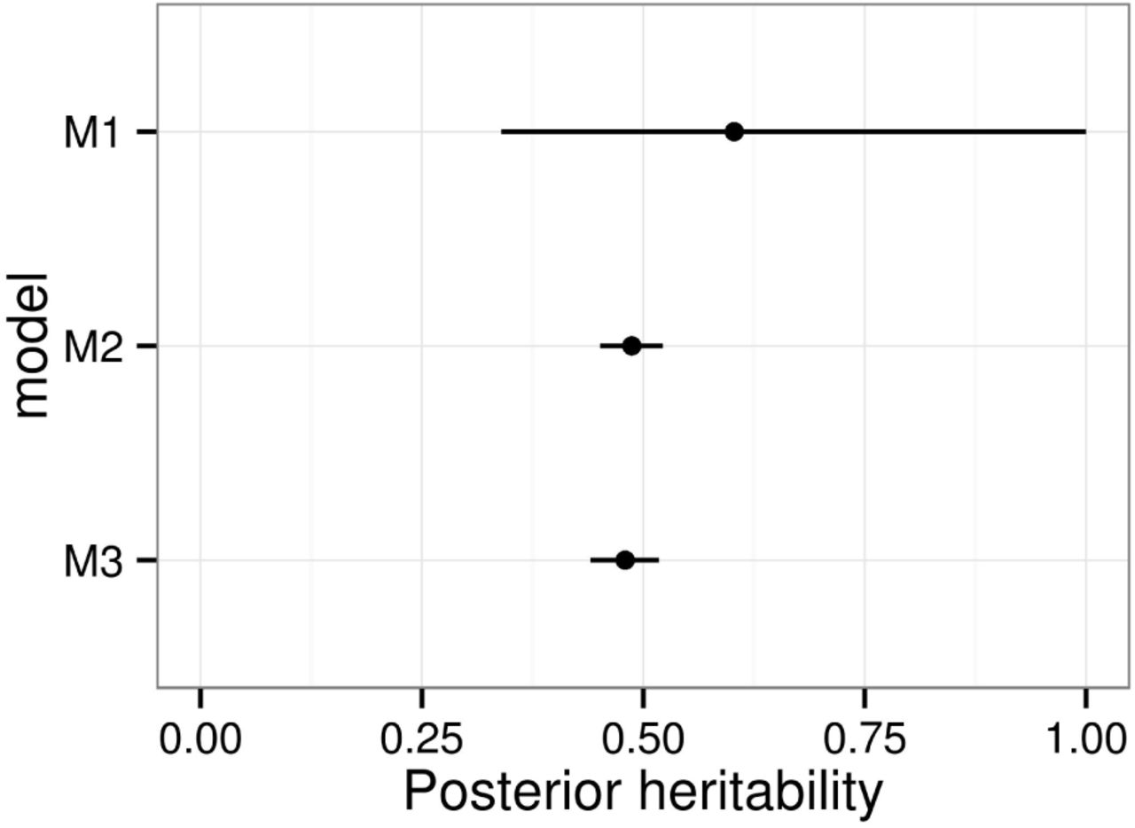
Posterior mean and 95% credible interval of narrow-sense heritability (h2) for crown dieback (CD) by model. The spatio temporal (ST) variance was excluded from the denominator in models M2 and M3.
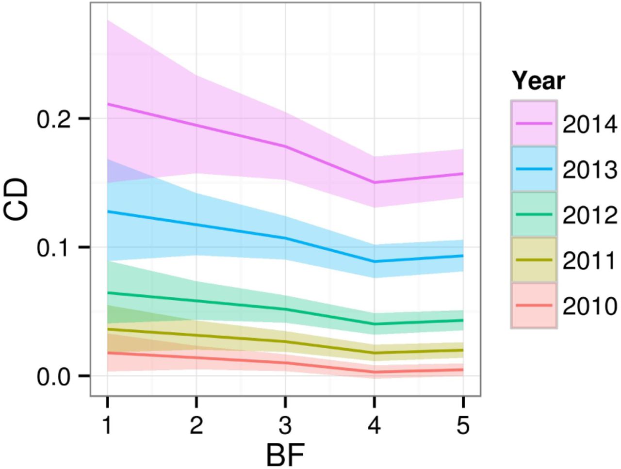
The fixed Year effect in model M5 reveals a clear progression of the disease, almost doubling the predicted CD value for a mean individual each year. Specific mean predicted values are 1.0%; 2.6%; 5.2%; 10.7% and 17.8%, although there is significant variability according to bud-flush precocity (Figure 8). Early flushers (high BF values) tend to have lower CD values.

Posterior mean and 95% Credible Intervals effect of budflush precocity (BF) on crown dieback (CD, original scale) by year.
The ST component in model M5 accounts for the dynamic spread of the disease, as a difference from the sustained increase in intensity captured by the Year effect. Figure 9 shows the posterior distributions of the range and variance of the Gaussian process and their corresponding priors. The fact that the posterior densities were concentrated well within the support of their corresponding prior indicates that the data were informative enough and the results were not constrained by the choice of the priors.

Prior and posterior densities for the spatial field characteristics for crown dieback (transformed: TCD). Range unit = spacing between trees.

Posterior mean spatio-temporal (ST) gaussian fields for crown dieback (transformed: TCD, low values refer to high susceptibility)

Posterior means and 95% Credible Intervals for the family effects from model M3.1 for crown dieback (transformed: TCD, families on the left are the most susceptible)
Figure @fig:st-maps shows the posterior mean spatio-temporal effect. When interpreting these maps it is important to recall that they do not represent the predicted spread of the disease, but only deviations from the global annual mean. Furthermore, the scale is inverted. So the disease in terms of CD seems to be consistently more intense in the bottom-left corner of the field.
The reparameterization of the model as in M5.1 allows to give estimates of the genetic merit of each family, and to compare the genetic variability between and within families. The posterior distribution of the variance between families is practically identical to that from model M1, while the predicted family effects are very similar except for some particular cases, notably family a04 which changes its position in the ranking (data not shown). Figure @fig:fam-posteriors shows the ranking of the families with respect to their estimated effect in model M5.1. However, even when there are remarkable differences among families, most of the genetic variability occurs within families (Figure 12). Specifically, the posterior modes and 95% HPD Credible Intervals are 0.040 (0.023, 0.081) for the variance between families and 0.136 (0.116, 0.155) for the variance within families. Consider for example families a09 and a10: although they are ranked in opposite extremes, the best individuals from a10 rank better than the worse individuals from a09 (data not shown).

Posterior modes and 95% HPD Credible Intervals of the variance components for crown dieback (transformed: TCD). The variances between and within families were computed from the alternative parameterization M5.1.
Although from Figure @fig:fam-posteriors it is evident that the mean effects of the families are significantly different, we specifically tested this hypothesis by fitting model M5.2 which forces all family effects to be equal to zero by imposing a sum-to-zero constraint in the breeding values for each family. This forces M5.2 to overfit the data as it turns out from the (almost double) effective number of parameters, which is comparable in magnitude with the total number of observations. Under these conditions the DIC and WAIC criteria are not reliable (Plummer 2008, Table 2). On the other hand, the marginal likelihood is considerably smaller meaning that model M5 is more likely than the model M5.2 which imposes a null variance between families.
Finally, the posterior modes and 95% HPD Credible Intervals are 0.137 (0.119, 0.156) for the additive-genetic variance and 0.147 (0.139, 0.157) for the residual variance. The narrow-sense heritability h2 is 0.42 (0.38, 0.47) or 0.48 (0.44, 0.52) if we excluded the ST variance from the denominator (Figure 7).
Modeling CL and estimating genetic parameters
Tables 3 and 4 present the selection criteria for the competing models of the binary and continuous components of the full model for CL, respectively. For the binary component, including the basal circumference improves DIC and WAIC, particularly in categorical form with an interaction with the Year. However, it worsens the Deviance. Suspecting some confusion with the ST effect (see Discussion), we decided not to include this variable in the final model. On the other hand, including a Provenance effect is clearly not relevant according to all these criteria. Analogously, neither the basal circumference nor the provenance improve the reference model for the continuous component.
Figure 13 shows the predicted versus the observed values for the binary and beta components of the mixture model. In the binary component, the predicted value corresponds to the probability of an outcome of zero (i.e., complete absence of collar lesion). Most of the observed zeros have a predicted probability greater than 0.5 while most of the trees with CL have a predicted probability of zero lower than 0.5. Thus, the model seems to provide a reasonable fit. For the continuous component, the model fit yields a prediction a bit shrinked due to the difficulty to predict values in the extremes for a bounded variable.

Fitted vs. observed values for the binomial (bin) and continuous (cont) components of the model for collar lesions (CL). The predicted parameter in the binary component is the probability of zero. Since the binary observations clump together in only two values, we improved the visualization using a violin plot, a modification of a box plot which represents a density estimation of the data.
Figure 14 represents the posterior IBV in the latent logit scale for the binomial component with respect to the infection status classified in four categories. Those who did not show any sign of infection got the highest predicted values, and therefore increased probability of an outcome of zero. On the other extreme, and as expected, the individuals that showed some level of infection both in 2012 and 2013 got the smallest BV. The degree of overlapping between these histograms indicates the relative importance of the genetic component with respect to the rest, as a predictor of the phenotype. This is related with the heritability which is presented below.

Distribution of individual breeding values (IBV) for the binomial component of collar lesions (CL, low values refer to high susceptibility), by observed infection status and history.
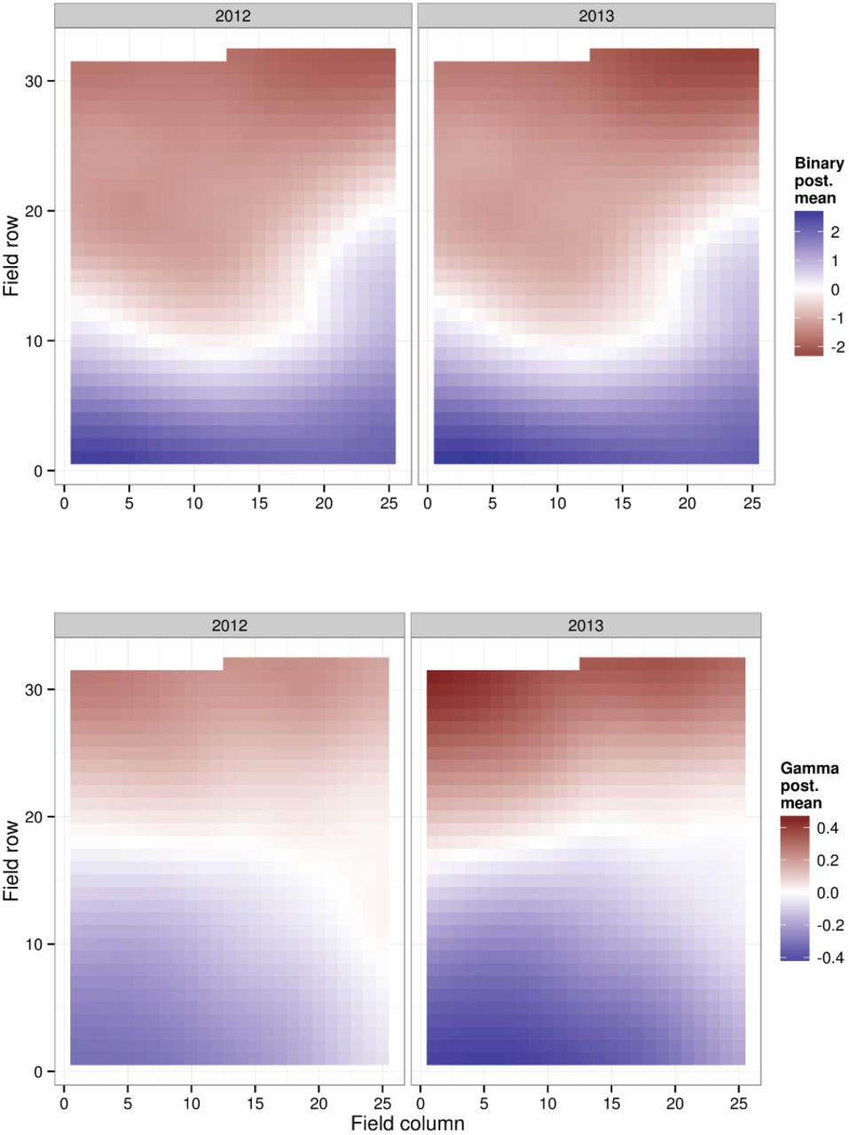
The ST effects display very clear trends (Figure 15). Particularly for the binary component, where the bottom rows show a higher-than-average probability of remaining uninfected in both 2012 and 2013. Similarly, when infected, trees in the top rows are likely to display higher CL values than average. The patterns for both years are very similar, in accordance with the high mean posterior interannual correlation estimates: 0.82 and 0.89 for the binary and beta components respectively.

Posterior mean spatio-temporal (ST) Gaussian fields for the binomial component (top) and the continuous component (bottom) of the model for collar lesions (CL), in the latent scale. Low values correspond to low susceptibility.

Prior and posterior densities for the spatio-temporal (ST) field characteristics of the binomial (bin) and continuous (cont) components of collar lesions (CL). Range unit = spacing between trees.
However, it should be noted that in contrast to the model for TCD, the prior distribution played a more significant role in the predicted spatiotemporal field, particularly for the binary component (Figure fig:cl-st-posteriors). This was expected, as spatially-distributed binary data is very little informative.
The mean posterior narrow sense heritabilities (h2) of CL are 0.49 and 0.42 for the binomial and continuous components respectively, with a slightly wider 95% Credible Interval for the binomial (0.32 - 0.64) than for the continuous (0.30 - 0.57) components. If the variance of the spatio-temporal term is excluded from the denominator, the posterior mean and Credible Interval for the heritability of the binomial component increase to 0.60 (0.48 - 0.71) (Figure 17).

Posterior means and 95% Credible Intervals of the narrow-sense heritability (h2) for the binomial (bin) and continuous (cont) components of collar lesions (CL) under two calculation methods: including (a) or not (b) the spatio-temporal (ST) variance in the denominator. For methodological reasons, the ST variance could not be excluded from the denominator for the gamma component.
Genetic correlation between both symptoms
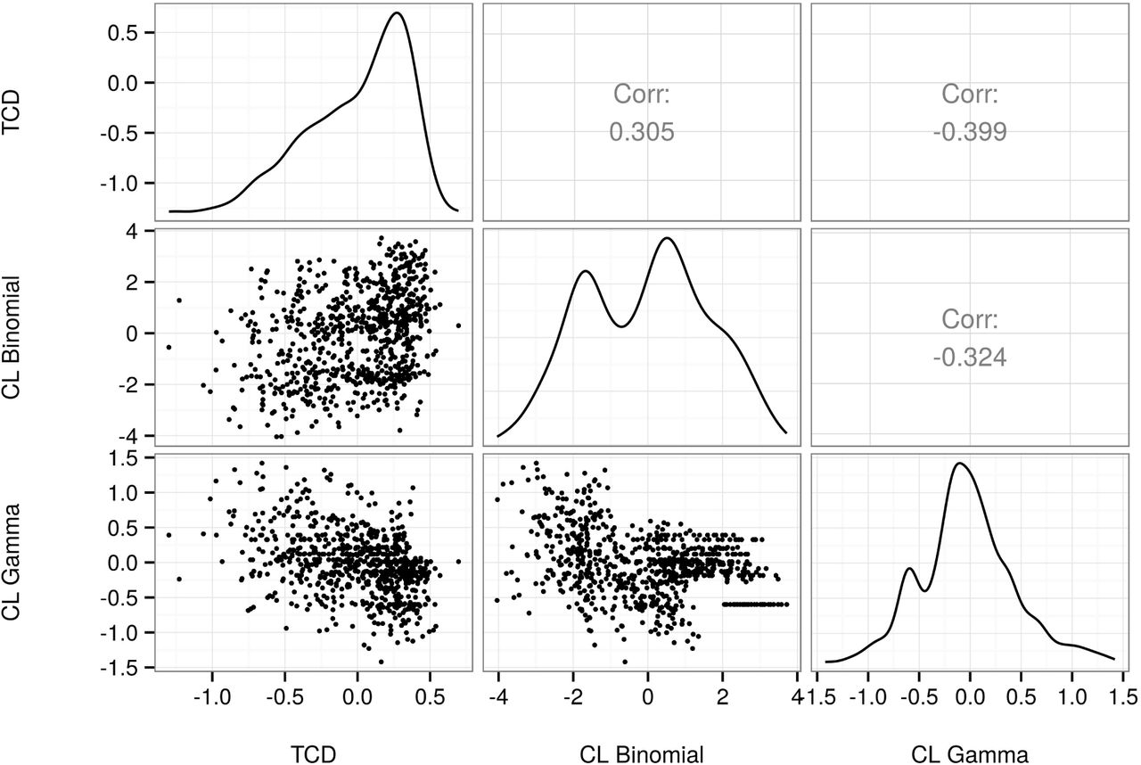
There seems to be a moderate negative correlation at genetic level between TCD and CL. The individuals with highest genetic merit for TCD (i.e. those who are predicted genetically better-suited to resist the disease symptom in the crown) tend to have higher predicted genetic resistance to the collar lesion, and lower predicted genetic sensitivity to it, in the case of infection (Figure 18).
Correlation between individual breeding values (IBV) for crown dieback (transformed: TCD, low values refer to high susceptibility) and the binomial (low values refer to high susceptibility) and continuous (low values refer to low susceptibility) components of collar lesions (CL).
Discussion
Disease progress and mortality
Trees were monitored over a four year period starting at the very onset of the disease. When reviewing the literature for the evolution of disease with time, finding figures on the proportion of symptomless or dead trees at a given point in time is easy. Indeed, mortality rates ranging from 2% to 70% have been reported (Enderle et al. 2013; Lobo et al. 2014; McKinney et al. 2014; McKinney et al. 2011; Metzler et al. 2012; Pliura et al. 2011; Pliura et al. 2014; Stener 2013). But very few studies allow to relate this rate to the time of exposure to the disease. Only three previous studies allow for comparisons, either because the trees started to be monitored for the disease right after planting or because initial proportions of symptomless tree suggest that the epidemics started only a short time before initial monitoring. Two of these studies found mortality rates higher to the 3% reported here despite similar times of exposure to the disease (9% in Enderle et al. 2013, 10% in Pliura et al. 2011). However, they both analyzed young trees (10 and 8 y.o., respectively, compared to 21 y.o. in the present study) and it is commonly accepted that there is a negative correlation between susceptibility to H. fraxineus and tree age (Skovsgaard et al. 2010). By contrast, another study (Pliura et al. 2014) reported a lower rate of 2% on very young trees (3 y.o.), but it was measured only one year after planting and on grafted material selected for resistance to the disease. Proportions of symptomless trees reported in the literature range from 1% (Lobo et al. 2014) to 58% (Kirisits et al. 2012). But again, comparisons should be made on trees of the same age that underwent similar exposure to the disease. One should also consider which symptoms were searched for before considering a tree healthy. In the present study, looking at CD only would yield a proportion of symptomless trees of 6% in 2014. However, already in 2013, more than 50% of the trees without visible CD had collar lesions. This result is in agreement with observations from Enderle et al. (2013) who found that 15% of otherwise healthy trees were affected by collar lesions. Removing trees without visible CD in 2014 but on which collar lesions were found the year before leads to a rate of asymptomatic trees of 4% only four years after first detection of disease.
Two studies at least have reported health improvement on some trees that restored a fraction of their crown (Lobo et al. 2014; Stener 2013). Indeed, a few percent of negative values were found for inter-annual increments for both CD and CL in the present study. A recovery processes may well act for CD, when secondary and epicormics shoots are produced in reaction to the disease thus providing the tree with more foliage. This process should be paid more attention when quantifying crown damage as these new shoots may have singular behavior in terms of phenology and susceptibility to the disease. Apparent remission in terms of CL may appear when basal girth of the tree increases more than the lesion(s), but the lack of precision in measuring CL may also explain part of this result. Indeed, at early stages, CL are often found below ground level and can be missed very easily. Moreover, basal girth is not a very repeatable measure due to the slope of the trunk at that level.
Collar lesions: still a lot to understand
In 2013, high proportions of trees showing only one of both symptoms demonstrate that they can occur independently. Nevertheless, and although not significant, a trend for a positive relationship between CD intensity and CL prevalence was observed at individual tree level both in 2012 and in 2013 (i.e. the two years when CL was investigated). This result is consistent with previous findings (Bakys et al. 2011; Enderle et al. 2013; Skovsgaard et al. 2010).
Severity of both traits were significantly positively correlated. Correlation at the phenotypic level has already been demonstrated by Bakys et al. (2011) who reported very high Pearson correlation coefficients (>0.57) between CD and several quantitative measurements of CL, and also by Husson et al. (2012) who reported Spearman correlation coefficients ranging from −0.2 to 0.7 in 60 natural plots with a tendency for higher correlation coefficients to happen in field plots with high overall mean CL. Using PCR assays, these authors also investigated the possibility that collar and branch lesions may be connected and did not find any evidence to support this hypothesis. Instead, they concluded on separate infection pathways with ascospores potentially infecting the stem base via lenticels in the bark. When analyzing the correlation between CL and CD, the causal component due to the fact that high CL values can cause CD symptoms just by preventing sap flow should also be taken into account.
There still are discussions about collar lesions being caused by H. fraxineus as the primary causal agent or not. The question will not be answered here as it would require in-deep molecular and histological investigations, but some results deserve attention. First, this study is first to provide estimates of the genetic correlation between both traits. The significant positive values reported here may indicate that both symptoms are due to the same pathogen with a least some common genetic determinism in the host. Of course, the possibility that resistance to H. fraxineus may also correlate with resistance to other collar-necrosis-inducing fungi cannot be excluded. Among those fungi, Armillaria sp. has been shown to occur at high frequency in ash collar lesions (Bakys et al. 2011; Husson et al. 2012; Lygis et al. 2005; Skovsgaard et al. 2010) and genetic variation for resistance to Armillaria has been demonstrated in at least one tree species (Zas et al. 2007). Interestingly, the genetic correlation coefficient was higher between CD and the gamma component of CL than with its binomial component. This is as expected in a scenario where H. fraxineus would induce the lesion while other fungi would be responsible for secondary decay. However, verifying this statement would benefit from measuring each lesion individually instead of expressing CL as a global girdling index.
Other interesting results arises when looking at the spatio-temporal dynamics of both symptoms. Looking at the effect of the distance to the nearest infected tree on the prevalence of both symptoms is consistent with the outputs from the modelling approach: the spatial correlation happens at much shorter range for CD than for both components of CL. The ST Gaussian field thus shows a patchy structure for CD while it fits a smooth surface for both CL components. Enderle et al. (2013) also observed significant spatial autocorrelation for CL prevalence and concluded on a strong indication that they are rather caused by Armillaria spp. which spreads via the soil or via diseased roots while H. pseudoalbidus would act as a more mobile secondary colonizer. Of course this hypothesis cannot be excluded here. This hypothesis could even explain why the ST Gaussian field is clearly biased towards susceptibility in the upper part of the field experiment for CL whereas it is the reverse for CD, at least from 2010 to 2013. The upper part of the field experiment is, indeed, adjacent to a forested land which can be considered a reservoir for Armillaria whereas the bottom part is close to an agricultural land (as a reminder, the whole experiment is installed in a former agricultural land). But these figures can also arise from other environmental factors such as soil moisture which has been shown to correlate with CL (Husson et al. 2012). This could explain why small basal girth correlates with lower CL prevalence and why including basal girth as a factor in the model for CL improved the DIC but decreased the likelihood of the model. Basal girth was found to exhibit significant spatial autocorrelation in this field experiment (data not shown) making it reasonable to say that its effect on CL is not biological but rather an indirect effect of local soil, and thus moisture, conditions.
Genetic components: their magnitude and how to estimate them properly
Only three studies explored the genetic variability of F. excelsior using OP progenies before this one (Kjaer et al. 2012; Lobo et al. 2014; Pliura et al. 2011). Among them, only one (Pliura et al. 2011) found significant Provenance effects. This outlying result may be due to the fact that these authors studied a large number of provenances (24) covering a large distribution range across Europe. However, as stated by the authors, the observed Provenance effect may simply originate from the fact that local (Lithuanian) provenances had undergone natural selection by the pathogen before mother trees were selected whereas other European provenances did not. Other studies, including this one, involved smaller numbers of provenances of local origins and did not conclude on significant Provenance effects.
All three previous studies concluded on significant Family effects and this is confirmed here. However, and because the analyzing method allowed computing both familial (= mother tree) and individual (= tree) breeding values in a straightforward manner, the present study allows to conclude that there is more genetic variation within families than between families.
Previous studies reported narrow-sense heritability estimates for CD in the range 0.20 – 0.92. However, the 0.92 estimate provided by Pliura et al. (2011) was based on a global health assessment and was apparently overestimated due to early frosts. The highest reliable h2 estimate is thus the one provided by Lobo et al. (2014), so that the published range of values is 0.20–0.49. In agreement with these figures, the present study concludes on an h2 estimate for CD of 0.42 and 95% HPD Credible Interval (0.45—0.52). For CL, h2 estimates were in the same range and cannot be compared to any data from the literature as this is the first time genetic variance components are estimated for this trait. In the sake of accuracy, it is important to point out that the heritability estimates provided here rely on the assumption that the studied families are composed of half-sibs only. They could be biased upwards should the average relatedness within progenies be higher. Checking this hypothesis would require intensive genotyping, and to our knowledge only Kjaer et al. (2012) conducted such verification. By reverse, our estimates should not be directly compared to those of Pliura et al. (2011) who computed them using an indirect estimation of the additive-genetic variance (i.e. four times the estimated variance of the Family effect), and a very particular definition of the phenotypic variance which takes into account only the Family and the residual variances disregarding the variability from the interaction between the family and the block. We, on the contrary, decided to keep this variance component in the denominator, thus leading to lower h2 estimates, as this is a recommended practice for a GxE component like this one (Visscher et al. 2008).
Interestingly, the analyzing procedure implemented here allowed generating h2 estimates with very narrow credible intervals. We believe such procedure (i.e. Bayesian analysis + explicit ST modelling) should be used whenever possible, especially when infection started recently, meaning that (i) measured traits are not normally distributed due to a high proportion of asymptomatic or low infected trees and (ii) disease escape can be confounded with resistance.
Although moderate, these heritability estimates are much higher than those reported in Ulmus for resistance to Ophiostoma novo-ulmi (i.e. 0.14 +/− 0.06, Solla et al. 2015), especially when considering that h2 was estimated at the intra-specific level here whereas the figures in Ulmus come from a mating design involving not only the European U. minor species but also the Central-Asian species U. pumila. Although DED is a true vascular disease whereas H. fraxineus is not, comparison between both pathosystems seems relevant because in both cases the tree host species is facing a previously unknown fungal pathogen and because some of the symptoms are similar (crown wilting). In the case of Ulmus, wilting has been shown to correlate with xylem vessel structure (Venturas et al. 2014) and exploring the relationship between resistance and anatomical features may be relevant in F. excelsior also. Understanding how the fungus develops inside the petiole and how it gets into the branch seems urgent.
Another relationship that was only partly explored here is the one between phenology and health status. In the case of Ulmus, percentage of wilting was negatively correlated with early bud flushing (Solla et al. 2015). In the case of F. excelsior, there are several indications that health status also correlates positively with early bud flushing but also with early leaf senescence and leaf coloring in the autumn (Bakys et al. 2013; McKinney et al. 2011; Pliura and Baliuckas 2007; Stener 2013). A significant positive correlation was found between early bud flushing and health status (CD) in the present study also. Although inoculation assays conducted by McKinney et al. (2012a) and Lobo et al. (2015) provided evidence that heritable stricto sensu resistance mechanisms occur in F. excelsior, some of the variability observed in the present study may thus come from phenological features leading to what should maybe termed ‘disease avoidance’. Although such features may prove valuable for selection, correlations between phenology and health status require further investigations as the disease can, in turn, modify the phenology of the host.
Consequences for management and breeding
The present study adds to the common perception that no complete resistance to H. fraxineus can be found in F. excelsior but that there is significant variability for partial resistance and that it is heritable. Whether partial resistance is preferable to complete resistance will not be discussed here. Some authors of this paper have experience with the poplar-rust pathosystem and know that partial resistance is not always a guarantee of durability (Dowkiw et al. 2010). Most importantly, confirming that there is heritable genetic variation for susceptibility in F. excelsior allows to believe that the species can be saved without introgressing resistance genes from exotic species like F. mandshurica, the supposed co-evolved host species of H. fraxineus. In addition to the many risks associated with exotic tree species, interspecific hybridization may prove a costly (due to the cost and time of backcrossing) and inadequate solution if the hybrids have growth, wood quality or other characteristics that do not meet the use of the species they are intended to replace.
Regarding natural regeneration, the positive consequence of moderate h2 estimates is that resistant F. excelsior trees that will remain or that will be reintroduced in natural populations will transmit resistance to the next generation in a highly additive manner. However, although we consider that this study reports on the heritability of resistance, this heritability is also that of susceptibility, meaning that highly susceptible trees will also transmit their behavior to the next generation. However, within family variation is so high that removing highly susceptible adult trees does not seem to be necessary except to avoid falling hazard. Promoting regeneration in natural stands and letting natural selection to occur may prove sufficient. Nevertheless, since selection by the pathogen will occur at the seedling stage, we must specify that this optimistic scenario may not come true if juvenile-adult correlations for resistance are low. These correlations have not been evaluated at the individual level yet, but juvenile trees are known to be more susceptible to the disease (Skovsgaard et al. 2010). This is undoubtedly due to their smaller architecture but maybe to singular anatomical, physiological or genetic features also.
For planting, high levels of intra-familial variation suggest that seed material from selected parents planted in seed orchards would require further selection. This could be done either in the nursery or directly in the field if planting is done at higher density than usual. Although not common for Ash (except for ornamental trees), clonal selection would certainly allow higher genetic gain. However, several questions would then arise. First is that of the number of clones to release to ensure sufficient genetic variability, not only to avoid resistance breakdown but also to cope with future threats like the Emerald Ash Borer (Agrilus planipenis) and to combine Ash dieback resistance with other traits of interest. Second is that of the techniques to use to propagate the selected Ash clones and the associated costs. F. excelsior is much easier to propagate through grafting than through cuttings. Although CL was found to be heritable in the present study, can we afford having two selection programs, one for rootstocks (CL resistance) and one for grafts (CD resistance)? Ash propagation through cuttings certainly deserves more investigation should clonal selection be considered.
It is important to keep in mind also that all genetic variance estimates, whatever their magnitude, were measured at a given point in time and in a given environment. H. fraxineus having a sexual stage, new variants of the pathogen appear each year and thus adaptation in the pathogen’s populations can occur. This may explain why significant GxE can be observed for resistance to H. fraxineus and why cloned (grafted) resistant material can become susceptible after only two growing seasons (Pliura et al. 2014). We are not aware of any field study where the genetic or the phenotypic (aggressiveness) variability of the pathogen was characterized but we definitely think developing tools to monitor the pathogen’s variability is a prerequisite to analyze the potential for durable resistance in any pathosystem.
Acknowledgements
This study was essentially supported by the French Ministry of Agriculture (Programme 149 – Action 13 – Sous action 32). F. Muñoz is partially funded by research grant MTM2013–42323-P from the Spanish Ministry of Economy and Competitiveness. We thank the town of Devecey for providing the land to install the field experiment and the technical team of INRA Nancy for their continuous commitment.
References


