

Abstract
The estimation of vital rates and life-history traits and how they vary with habitat and population factors are central for our understanding of population dynamics, risk of extinction, and evolution of traits in natural populations. We used long-term tag-recapture data and novel statistical and modeling techniques to investigate how population and environmental factors determine variation in vital rates and population dynamics in the population of brown trout Salmo trutta L. of Upper Volaja (Western Slovenia). Alien brown trout were introduced in the stream in the 1920s and the population has been self-sustaining since then. The population of Upper Volaja has been the subject of a monitoring program that started in 2004 and is currently on going. Upper Volaja is also a sink, receiving individuals from a source population living above an impassable waterfall. We estimated the contribution of the source population on the sink population and tested the effects of temperature, population density, and early environment on variation in vital rates and life-history traits among more than 4,000 individually tagged brown trout that have been sampled since 2004. We found that fish migrating from the source population (>30% of population size) help maintain high population densities despite poor recruitment. Neither variation in density nor in temperature explained variation in survival or growth; the best model of survival for individuals older than juveniles included cohort and time effects. Fast growth of older cohorts and higher population densities in 2004–2006 suggest very low densities in early 2000s, probably due to a flood event that caused a strong reduction in population size. Higher population densities, smaller variation in growth and weaker maintenance of size hierarchies with respect to endemic marble trout suggest that exploitative competition for food is at work in brown trout and interference competition for space is operating in marble trout.
1 Introduction
The way that vital rates and life histories in a population or species change in space and time and the consequences of this variation for population dynamics and risk of extinction are central topics in ecology (Frederiksen et al. 2014). With unprecedented rates of climate (e.g. mean and variance of temperature, precipitation) and environmental change (e.g. habitat fragmentation or destruction, pollution), it is urgent to develop powerful methods for analysis and test hypothesis on the relationship between populations and environment that can help us predict future species’ response and implement effective conservation measures for threatened species.
Due to the large number of potential determinants and individual and group heterogeneity in responses, understanding how variation in habitat factors drives variation in traits and population dynamics is intrinsically difficult (Elliott 1994, McCallum 2000). This task can be further complicated by small population sizes, demographic stochasticity, and the occurrence of stochastic – and potentially unobserved – environmental and climatic events. Understanding the potential effects of habitat factor on vital rates, life histories, and population dynamics is a subject best approached by a combination of theoretical and empirical methods in which the empirical work guides the theoretical constructs and the modeling identifies key pieces of empirical information that are required for advancing understanding (Vincenzi and Mangel 2014).
Within a population, habitat factors, both extrinsic (e.g. weather, predators or food availability) and intrinsic (e.g. population density or composition) (Aars and Ims 2002) and their interaction (Baerum et al. 2013), determine a large part of the temporal variation in the distribution of vital rates, recruitment, and population dynamics (Jonsson and Jonsson 2011). Individual heterogeneity contributes to explain part of the variation and increases the variance in vital rates (Vindenes and Langangen 2015). Organisms living in the same population often differ in the ability to acquire resources, in their life-history strategies, and in their contribution to the next generation (Lomnicki 1988, Vindenes and Langangen 2015). These differences may result from complex interactions between genetic, environmental, population factors, and chance, and can have substantial consequences for both ecological and evolutionary dynamics (Pelletier et al. 2007, Coulson et al. 2010, Vindenes and Langangen 2015). When not accounted for, the presence of substantial individual variation can affect the estimation of vital rates and other demographic traits for use in population and life-history models, which may translate to wrong predictions of those models and wrong inference on co-variation among vital rates (Pfister and Stevens 2003, Coulson et al. 2009, Smallegange and Coulson 2013, Vincenzi et al. 2014b, 2015).
In addition to the intrinsic biological and computational complexities associated with the estimation of variation in vital rates, taking into account individual heterogeneity further increases the complexity of model specification and parameter estimation (Thomson et al. 2009, Ford et al. 2012, Laake et al. 2013, Vincenzi et al. 2014b). Longitudinal data (e.g. tag-recapture) facilitate the estimation of individual and group (i.e. sex, year-of-birth cohort) variability in life-history traits and fitness (Thomson et al. 2009). However, when fine-grained data on individuals and habitat factors are available, the choice of the hypotheses to be tested is critical, since the testing of a large number of hypotheses increases the chances of finding spurious correlations among responses and potential predictors (Simmons et al. 2011, Head et al. 2015).
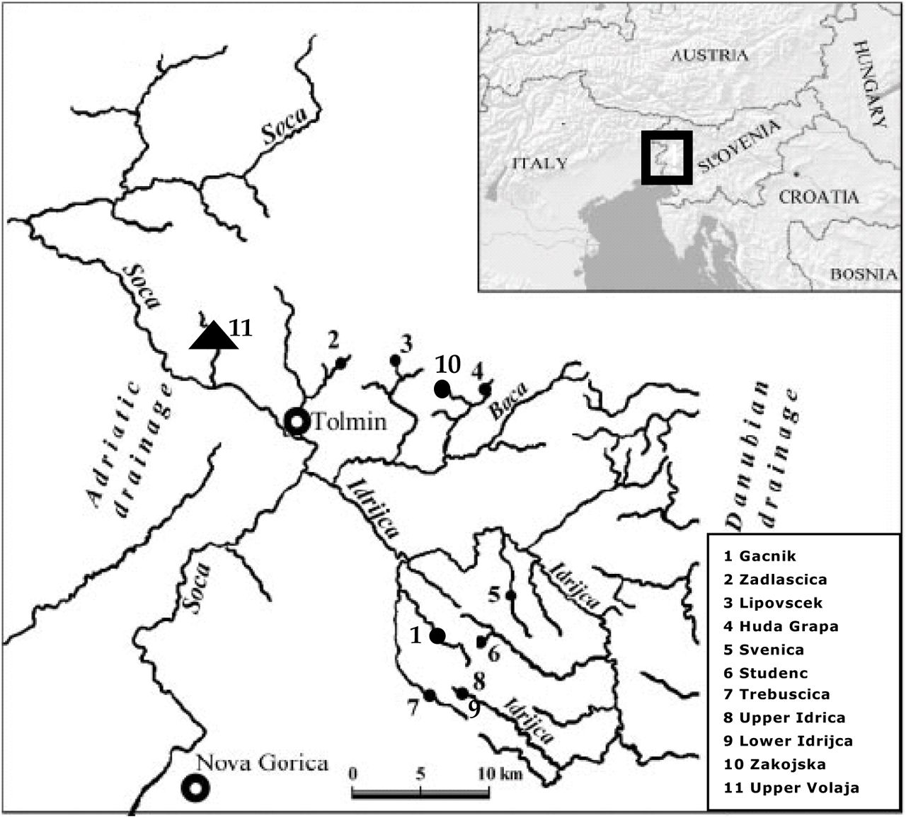
Salmonids have been often used as model systems in ecology and evolutionary biology, due to their ample geographic distribution, their ecological and life-history variability (both within-and among populations), and their strong genetic and plastic responses to habitat variation (Elliott 1994, Stearns and Hendry 2003, Garcia de Leaniz et al. 2007, Jonsson and Jonsson 2011). In this work, we combined an exceptional long-term tag-recapture dataset and powerful statistical methods to identify the determinants of variation in vital rates among years, groups and individuals of a introduced population of brown trout living in Upper Volaja (Western Slovenia), as well to understand how the effects of that variation influence the population dynamics of the species. The population of Upper Volaja was created in the 1920s by stocking brown trout Salmo trutta L. and it has been self-sustaining since then. A monitoring program started in 2004 to investigate the Upper Volaja brown population, with the goals of understanding the ecology of this unique populations and of testing differences between traits and population dynamics of alien brown trout and endemic, charismatic marble trout living in the same area and in similar environments (Vincenzi et al. 2015) (Fig. 1).

Populations of marble trout (dots) and brown trout (triangle) living in Western Slovenia. The populations of Zajojska and Gacnik were newly created in 1996 and in 1998, respectively.
The ten remnant, genetically pure marble trout populations living in Western Slovenia have been intensively monitored and studied since 1993. Marble trout populations are highly genetically differentiated (Fumagalli et al. 2002), persist at low population densities (between ~600 and 1250 fish ha−1 for fish older than young-of-year), are at high risk of extinction due to flash floods and debris flows (Vincenzi et al. 2008c, 2015), and show a fast-to-slow continuum of life histories, with slow growth associated with higher survival at the population level, possibly determined by food conditions and the effects of sexual maturity (at younger age in faster-growing populations) on survival (Vincenzi et al. 2015). In marble trout, mean annual probability of survival from fish older than young-of-year ranged from 0.33 (population of Lower Idrijca) to 0.62 (Huda Grapa) (Vincenzi et al. 2015). Marble and brown trout can interbreed (Berrebi et al. 2000, Meldgaard et al. 2007), they are phylogenetically close (Crête-Lafrenière et al. 2012, Lamaze et al. 2012), but there are no comparative studies on differences in their ecology, including type of intra-specific competition for resources (Ward et al. 2007, Le Bourlot et al. 2014), vital rates and population dynamics.
The brown trout population of Upper Volaja is enclosed between two impassable waterfalls and receives fish from a un-sampled population living upstream; it is thus a “source-sink system”, in which the dynamics of the population of Upper Volaja depends not solely on its internal demography, but also on the input of individuals from the population living above the waterfall (Dias 1996). Specifically, we estimated the contribution of the source population on the sink population and tested the effects of temperature, population density, and early environment on variation in vital rates and life-history traits (growth, survival, movement, recruitment) among more than 4,000 individually tagged brown trout that have been sampled between 2004 and 2015. We then investigated differences between brown trout and marble trout living in the same environment and advanced hypothesis on the ecological processes determining those differences. Our work also provides a framework for the fine-grained estimation of vital rates and life-history traits when there is substantial individual and shared variation in those traits, and highlights the importance of long-term studies in ecology (Elliott 1994).
2 Material and Methods
2.1 Species and study area
The first documented introduction of brown trout in Western Slovenia occurred in 1906 (Gridelli 1936); in the following decades, a large proportion of the lower reaches of Western Slovenian streams were stocked with brown trout (Berrebi et al. 2000, Meldgaard et al. 2007). As a measure for the conservation of the endangered and charismatic marble trout (Crivelli et al. 2000), the stocking of alien brown trout in Western Slovenian streams has been prohibited since 1996 (Razpet et al. 2007). The biology and life histories of brown trout are generally well known (Elliott 1994, Jonsson and Jonsson 2011). Brown trout live in well-oxygenated waters; the limits for growth in this species are 4–19.5 °C, the lower limit for survival is 0 °C and the upper limit varies between 25 °C and 30 °C depending upon the acclimation temperature. Limits for egg development are narrower at about 0–15 °C (Elliott 1994). Brown trout can be freshwater resident or can migrate to sea, lakes, or estuaries (Elliott 1994). Mortality is usually high during the first few weeks after emergence. Depending on growth and life histories, resident brown trout achieve sexual maturity anywhere from 1 to 10 years. In the Northern Hemisphere, the usual time for breeding in most populations is between November and January (Riedl and Peter 2013) and brown trout may spawn over several years.
The monitored population of resident brown trout of Upper Volaja lives in a stretch of stream approximately 265 m in length that is enclosed between two impassable waterfalls (Table S1). The catchment is pristine and there are neither poaching nor angling in the stream. Brown trout is the only fish species living in Upper Volaja. Fish can migrate from the upstream part of the population (a source population for Upper Volaja) into Upper Volaja and from Upper Volaja into the downstream population (which is thus a sink for the upstream population(s)). Due to the harsh and prohibitive environment, sampling has never been conducted above (AW from now on) and below (BW) the waterfalls enclosing Upper Volaja, although we know that the population of brown trout in AW extends for ~400 m. Within Upper Volaja, there are no physical barriers impairing upstream or downstream movement of brown trout; however, brown trout are territorial and their movement throughout their lifetime is typically limited (Vøllestad et al. 2012).
2.1.1 Sampling
We sampled the population of Upper Volaja bi-annually in June and September of each year from September 2004 to September 2015 for a total of 23 sampling occasions. Fish were captured by electrofishing and length (L) and weight recorded to the nearest mm and g, respectively. If captured fish had L > 115 mm, and had not been previously tagged or had lost a previously applied tag, they received a Carlin tag (Carlin 1955) and age was determined by reading scales. Fish are aged as 0+ in the first calendar year of life, 1+ in the second year and so on. Sub-yearlings are smaller than 115 mm in June and September, so fish were tagged when at least aged 1+. The adipose fin was also removed from all fish captured for the first time (starting at age 0+ in September), including those not tagged due to small size at age 1+. Therefore, fish with intact adipose fin were not sampled at previous sampling occasions at age 0+ or 1+. Males and females are morphologically indistinguishable in either June or September, thus trout were not sexed. Fish were also assigned a sampling location (sector) within Upper Volaja. Sectors were numbered from 4 (most upstream) to 1, with sector 4 being the longest (95 m) and sector 1 the shortest (45 m) (Table S1).
2.1.2 Environmental data
Annual rainfall in the meteorological station closest to Upper Volaja (Vogel, Slovenia) was recorded as between 2000 and 3600 mm between 1983 and 2013. An ONSET temperature logger recorded mean daily water temperature in Upper Volaja. Missing water temperature data in 2004 (all year) and 2005 (from January 1st to June 10th) were estimated using water temperature recorded in the stream Lipovscek (Pearson’s r = 0.98 over 2004 to 2014 daily water temperature data).
We used water temperature data to calculate growing degree-days (GDDs) with the formula GDD = Tmean − Tbase, where Tmean is the mean daily water temperature and Tbase is the base temperature below which growth and development are assumed to stop. We set Tbase at 5 °C as it is the lowest temperature at which brown trout grow according to Elliott et al. (1995). GDDs are the sum of the days in which growth is possible during a specific time period (Chezik et al. 2014). Annual GDDs and mean annual T showed very little variation from 2004 to 2014 (mean±sd GDDs = 1204.94±115.71, CV = 9%; T = 8.37±0.21, CV = 3%) (Fig. S1). Water flow rates have never been recorded in Upper Volaja. A full list of abbreviations used in this paper is in Table S2.
2.2 Density and movement
We estimated density of 0+ fish only in September, since fish emerged a few days before the June sampling. We estimated density of fish older than 0+ for age, size-class, or cohort using a two-pass removal protocol (Carle and Strub 1978) as implemented in the R (R Development Core Team 2014) package FSA (Ogle 2015). Total stream surface area (746.27 m2) was used for the estimation of fish density (in fish ha−1). We assessed the contribution of trout from AW (source) to Upper Volaja (sink) by estimating for each year of sampling the proportion of fish that were not sampled in Upper Volaja either at 0+ in September or 1+ in June. Fish with adipose fin cut were assumed to be born in Upper Volaja or be early incomers (that is, fish migrating into Upper Volaja when younger than 1+ in September), while fish with intact adipose fin were assumed to be born in AW and be “late incomers”, that is fish migrating into Upper Volaja when 1+ in September or older. We grouped together fish born in Upper Volaja and early incomers (“early incomers” from now on), since we cannot distinguish between them (see Text S1 for full details). We tested for recruitment-driven population dynamics by estimating correlations between density of 0+ fish (D0+) in September and density of older than 0+ (D>0+) one or two years later.
For movement, we estimated the proportion of tagged trout sampled in different sectors at different sampling occasions. Then, we estimated the parameters of a Generalized Linear Model (GLM) in which the number of different years in which a fish was sampled predicted the probability of a fish being sampled in different sectors.
2.3 Growth and body size
In order to characterize size-at-age and growth trajectories, we modeled variation in size at first sampling (i.e. 0+ in September), individual and year-of-birth cohort lifetime growth trajectories, and growth between sampling occasions. Much of the literature on growth in wild brown trout focuses on mass (and typically finds that brown trout in nature grow slower than in the laboratory when temperature is optimal and food is provided ad lib (Elliott et al. 1995, Elliott 2009)). However, we focused on length, since it is more closely related to reproductive traits and it allows a comparison with growth of marble trout living in the same area (Vincenzi et al. 2014b, 2015).
2.3.1 Variation in size at age 0+
We used an ANCOVA model to model the variation in mean length of cohorts at age 0+  using D>0+ and GDDs (up to August 31st) and their interaction as candidate predictors. Following Vincenzi et al. (2008a, 2010b) and studies on density dependence of growth in salmonids (summarized in Jonsson and Jonsson 2011), we log-transformed both
  and D>0+. We carried out model selection with the MuMIn package (Barton 2013) for R, using the Akaike Information Criterion, AIC (Akaike 1974, Symonds and Moussalli 2010) as a measure of model fit. We considered that models had equal explanatory power when they differed by less than 2 AIC points (Burnham and Anderson 2002).
2.3.2 Lifetime growth trajectories
The standard von Bertalanffy model for growth (vBGF; von Bertalanffy 1957) is where L∞ is the asymptotic size, k is a coefficient of growth (in time−1), and t0 is the (hypothetical) age at which length is equal to 0.
We used the formulation of the vBGF specific for longitudinal data of Vincenzi et al. (2014b), in which L∞ and k may be allowed to be a function of shared predictors and individual random effects.
In the estimation procedure, we used a log-link function for k and L∞, since both parameters must be non-negative. We set where u ~ N (0,1) and v ~ N (0,1) are the standardized individual random effects, σu and σv are the standard deviations of the statistical distributions of the random effects, and the other parameters are defined as in Eq. (2.1). The continuous predictor xij (i.e. population density or temperature, as explained below) in Eq. 2.2 must be static (i.e. its value does not change throughout the lifetime of individuals).
We thus assume that the observed length of individual i in group j at age t is where εij is normally distributed with mean 0 and variance
  .
.
Since the growth model operates on an annual time scale and more data on tagged fish were generally available in September of each year, we used September data for modeling lifetime growth. Following Vincenzi et al. (2014b, 2015), we included three potential predictors of k and L∞: (i) cohort (Cohort) as a group (i.e. categorical) variable (α1 and β1 in Eq. 2.2), (ii) population density (fish older than 0+) in the first year of life (D>0+,born) as a continuous variable (i.e. xij Eq. 2.2), and (iii) GDDs in the first year of life as a continuous variable.
In addition, we tested the hypothesis of a longitudinal gradient in growth within Upper Volaja - as commonly found in marble trout living in the study area (Vincenzi et al. 2014b) - in which fish living more upstream show higher length-at-age than fish living more downstream, probably due to more food drift available to them. Thus, we also used (iv) sampling sector as categorical predictor of k and L∞.
Datasets for the analysis of lifetime growth trajectories
When using shared k and L∞ among all fish in a population (i.e. no predictors for either k or L∞) or when using Cohort as their predictors we used the whole tag-recapture dataset for Upper Volaja (datasets DataW).
There were fish in every population that were born before both D>0+,born and temperature data were available. For instance, the oldest fish sampled in Upper Volaja was born in 2000, but D>0+,born and water temperature were first estimated and recorded in 2004. Since we wanted to compare the explanatory power of the growth models when D>0+,born, GDDs, Cohort, were used as predictors of vBGF’s parameters, we used a subset of the whole datasets (datasets DataD) when using D>0+,born and GDDs as potential predictors. In each analysis, we used AIC to select the best model.
As the inclusion of trout captured in different sectors throughout their lifetime would not allow using sampling sector as predictor of vBGF’s parameters in the formulation in Eqs (2.2.) and (2.3), when using sampling sector as predictor we used a subset of the DataW (DataS) that included (a) trout that were sampled once at age 1+, and (b) trout that were sampled multiple times in the same sector and were sampled for the first time at age 1+ (the latter due to avoid bias introduced by fish coming into Upper Volaja from AW, thus by fish that had grown for years in a different environment). Although we cannot exclude that fish sampled multiple times in the same sampling sector had moved between sectors outside the days of sampling, given the limited movement of brown trout we assumed that, in case of (b), trout stayed permanently in the same sector. When using sampling sector as predictor, we only analyzed model results without comparing model fit to other model formulations.
2.3.3 Growth in size between sampling intervals
We used Generalized Additive Mixed Models (GAMMs) (Zuur et al. 2014) to model variation in mean daily growth Gd (in mm d−1) between sampling occasions using length L, Age, GDDs over sampling intervals by Season, and D>0+ as predictors, plus fish ID as a random effect. Since we expected potential non-linear relationships between the two predictors and Gd, we used candidate smooth functions for L and GDDs. We carried out model fitting using the R package mgcv (Wood 2011) and model selection as in Section 2.3.1.
2.4 Recruitment
Brown trout living in Upper Volaja spawn in December-January and offspring emerge in June-July. Females achieve sexual maturity when bigger than 150 mm, usually at age 2+ or older, and can be iteroparous (Meldgaard et al. 2007, Vincenzi et al. 2014a). We used density of fish with L > 150 mm as density of potential spawners at year t (Ds,t). We used density of 0+ in September of year t as a measure of recruitment (Rt). We used Generalized Additive Models (GAMs) (Wood 2006) to model variation in Rt using density of potential spawners in September of year t−1 (Ds,t−1) and GDDs for year t up to emergence time (we assumed from January 1st to May 31st for standardization purposes) as predictors. We used candidate smooth functions for GDDs and Ds,t-1 as we were expecting potential non-linear relationships between the two predictors and Rt. We carried out model selection as in Section 2.3.1.
2.5 Survival
To characterize variation in survival and identify the determinants of this variation, we modeled survival between sampling occasions for tagged fish and survival between age 0+ and 1+ for untagged fish that were first sampled in the stream when 0+.
2.5.1 Survival of tagged individuals
Our goal was to investigate the effects of mean temperature, early density, season, age, and sampling occasion on variation in probability of survival of tagged fish using continuous covariates (D>0+, mean temperature between sampling intervals  , Age) at the same time of categorical predictors (Cohort, Time, Season). Since only trout with L > 115 mm (aged at least 1+) were tagged, capture histories were generated only for those fish. Full details of the survival analysis are presented in Text S2.
Two probabilities can be estimated from a capture history matrix: ϕ, the probability of apparent survival (defined “apparent” as it includes permanent emigration from the study area), and p, the probability that an individual is captured when alive (Thomson et al. 2009). In the following, for ϕ we will simply use the term probability of survival. We used the Cormack–Jolly–Seber (CJS) model as a starting point for the analyses (Thomson et al. 2009). We started with the global model, i.e. the model with the maximum parameterization for categorical predictors. From the global model, recapture probability was modeled first. The recapture model with the lowest AIC was then used to model survival probabilities.
We modeled the seasonal effect (Season) as a simplification of full time variation, by dividing the year into two periods: June to September (Summer), and the time period between September and June (Winter). As length of the two intervals (Summer and Winter) was different (3 months and 9 months), we estimated probability of survival on a common annual scale. Both Age and  were introduced as either non-linear (as B-splines, Boor 2001) or linear predictors, while D>0+ was introduced only as a linear predictor. In addition, we tested whether probability of survival of trout that was born in AW was different from that of fish born in Upper Volaja. In this case, we used a subset of the whole dataset that included cohorts born between 2004 and 2010. We carried out the analysis of probability of survival using the package marked (Laake et al. 2013) for R.
2.5.2 Survival from age 0+ to 1+ (first overwinter survival)
Because fish were not tagged when smaller than 115 mm (thus 0+ were not tagged), we assumed a binomial process for estimating the probability σ0+ of first overwinter survival (0+ in September to 1+ in June) for trout that were sampled in September of the first year of life and had the adipose fin cut (see Text S3 for details on the estimation of σ0+). This way, immigration of un-sampled individuals at 0+ will not influence the estimated survival probabilities. We tested for density-dependent survival σ0+ by estimating a linear model with D>0+,m (mean of D>0+ at year t in September and t+1 in June) as predictor of the estimate of  . Following Vincenzi et al. (2008b, 2010b), we log-transformed both
  and D>0+,m. We carried out model selection as in Section 2.3.1.
3 Results
3.1 Variation in density, recruitment, and movement
The estimated probability of capture at every depletion pass was very high (mean±sd of point estimates across sampling occasions: 0.86±0.07 for 0+ fish and 0.91±0.02 for fish older than 0+) (Table S3). Population density was variable through time, although the coefficient of variation (CV) was low for D>0+ (15%) and high for D0+ (65%) (Fig. 2 and Table S3). The estimated number of trout in the stream was between (mean±se) 0 (2014) and 65±1.4 (2015, 871±19 fish ha−1) for 0+ and between 327±1.9 (2015, 4382±25 fish ha−1) and 548±2.9 (2004, 7343±38 fish ha−1) for older fish (Fig. 2 and Table S3). For each cohort born after the start of sampling (i.e. the first cohort sampled at 0+ was the one born in 2004), the number of fish in a cohort noticeably increased after the first sampling (i.e. from 0+ to 1+), thus showing a substantial contribution of fish from AW to population size and population dynamics of brown trout in Upper Volaja (Fig. 2). Since 2010 (the first year in which fish from cohorts born before 2004 were fewer than 10% of population size), the proportion of trout alive that were not sampled in Upper Volaja early in life (i.e. “late incomers”) has been high and stable across years (0.35±0.05, Table S4).

Density over time of brown trout aged 0+ (dashed black line), older than 0+ (solid black line), and single year-of-birth cohorts (from C04 = 2004 to C10 = 2010) in September. 95% confidence intervals are barely visible as the probability of fish capture at each passage was very high (~90%) and consequently confidence intervals very narrow. The density of cohorts increased in the first year (and sometimes for two years) after the year of birth due to input from the population living above the waterfall (AW).
There was little variation in density of potential spawners across years (mean±sd = 3459±442 fish ha−1, CV = 13%). The best model of recruitment Rt did not include either GDDs or Ds,t-1. The best models with GDDs (negative effect, ΔAIC = 2.86) and Ds,t-1 (positive effect, ΔAIC = 3.41) were poorly supported by data. We observed complete recruitment failure in 2014, despite an average density of potential spawners sampled in September 2013 (3270±21 fish ha−1). The estimated number of 1+ in September 2014 (thus all fish coming from AW after September 2014) was 20±0.8.
There was no significant lagged correlation (either for lag of 1 or 2 years) between D0+ and D>0+, which indicates that recruitment (density of 0+ in September at year t) was not driving variation in population density of fish older than juveniles at year t + 1 or t + 2. The oldest brown trout sampled in Upper Volaja was 12 years old and most of brown trout died before reaching 6 years of age (Fig. S2).
Only 26±1% of tagged fish were sampled in more than one sector across sampling occasions. Of those, ~25% were sampled at different sampling occasions in non-adjacent sectors. The probability of being sampled in different sectors increased with the number of years in which a fish was sampled (GLM, α = −0.04±0.02, β = 0.13±0.01 (p<0.01)).
3.2 Growth and recruitment
The best model for mean length of age 0+ fish  in September had only D>0+ as predictor (negative effect, R2 = 0.28, p = 0.06), although models with only GDDs (positive effect of GDDs, ΔAIC from best model = 0.61) or no predictors (ΔAIC = 0.78) had basically the same explanatory power of the best model.
Empirical growth trajectories for tagged fish (i.e. L > 115 mm) in September (n = 4590; n of cohorts between 7 [cohort 2000] and 370 [2003]) showed individual variation in growth rates and size-at-age (Fig. 3 and Fig. S3), thus supporting the choice of a growth model with individual random effects. The biggest brown trout sampled in Upper Volaja was had L = 297 mm when 7 years old (Fig. S3). The best growth model for brown trout had Cohort as a predictor of both L∞ or k (Table S5), although the effect size of the difference in growth among cohort was small, in particular for cohorts born after 2003 (Fig. 3 and Table S6).

Average growth trajectories of brown trout (individual random effects for L∞ and k set to 0) living in different cohorts along with 95% confidence intervals of the average trajectories. Thin lines and dots are growth trajectories and length-at-age data of fish born in 2000 (black solid), 2001 (gray solid), 2010 (black dashed). Trout born after 2004 had similar cohort-specific growth trajectories, with confidence intervals of the average trajectories largely overlapping (see Table S6).
When using DataD (i.e. also including GDDs and D>0+,born as predictors of k and L∞), the best models were the same as those found when using DataW. The best model including D>0+ and/or GDDs introduced an additive effect of D>0+ and GDDs on both L∞ or k; for L∞, both D>0+ and GDDs had a negative effect, while there was a positive effect of both variables on k. We found a longitudinal gradient in lifetime growth in Upper Volaja, with fish sampled in sampling sectors more upstream growing faster and having larger asymptotic size than fish sampled in more downstream sectors. However, differences were small and confidence intervals for the average growth trajectories tended to overlap (Fig. 4 and Table S7).

Average growth trajectories in sampling sectors for brown trout that have been sampled either once at age 1+ or multiple times in the same sampling sector (with first sampling occurring at age 1+). Brown trout tend to grow faster in sampling sectors more upstream (S4 is the most the upstream sampling and S1 the most downstream).
Brown trout relatively large early in life tended to remain larger than their conspecifics throughout their lifetime (Pearson’s r of size at age 1+ and size at age 3+ = 0.25, p < 0.01). The best model of growth between sampling intervals included Cohort, Age (growth tended to be slower at older ages), L (growth decreased with increasing L), and the interaction between density and Season as predictors of mean daily growth Gd (n = 4174, R2 = 0.33; Fig. S4). GDDs had a positive, although small, effect on Summer growth and a negative and stronger effect on Winter growth (Fig. S4). The growth model was not able to predict the growth spurts occasionally experienced by some fish, which were probably due to a switch to cannibalism (Fig. 5).

Observed daily growth (in mm d−1) and daily growth predicted by the best growth model for fish aged 1+ (left panel) and fish older than 1+ (right panel). Gray: June-to-September growth. Black: September-to-June growth (see Fig. S4 for the smooth functions of the GAMM).
3.3 Survival
We found a highly variable probability of early survival σ0+ over years, ranging from 0.1 to 0.62 on an annual temporal scale. The best model for σ0+ included only D>0+,m as predictor, with ~28% of the variation in early survival that was explained by the model. Contrary to what is commonly observed, the effect of D>0+,m on σ0+ was positive (Fig. 6).
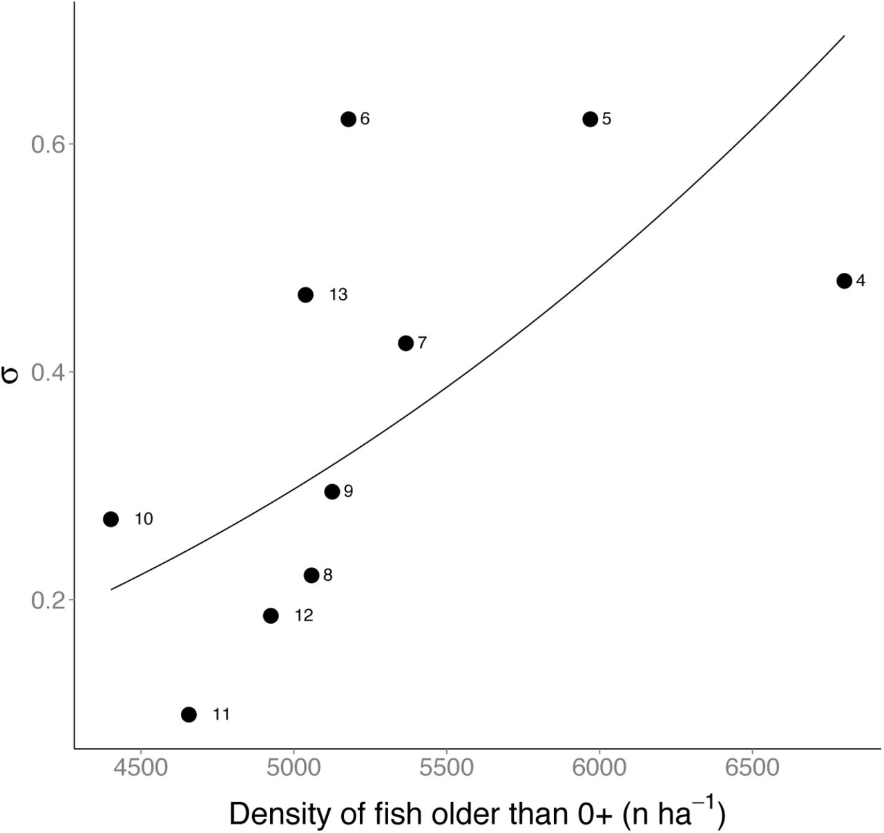
The best model for probability of early survival σ0+ included a positive effect of D>0+,m (linear model on log-log scale: α = −24.76±11.06, β = 2.76±1.30,  , p = 0.06). The labels identify the year of birth of fish (e.g. 4 = survival from 0+ to 1+ of the 2004 cohort).

Probability of survival (mean and 95% confidence intervals) on an annual temporal scale with the model with additive effect between Cohort and Time (best model, left panel), model with Time effect (center panel), and model with Density of fish older than 0+ ( D>0+) effect (left panel). For Cohort and Time, the last survival estimate is not reported as for each cohort the 95% confidence intervals were between 0 and 1.
Probability of capture for tagged brown trout was very high (p = 0.84 on average across sampling occasions); in the best capture model for tagged trout, the probability of capture depended on sampling occasion (Table S8). The best model for probability of survival had an additive effect of Cohort and Time on ϕ (Table 1 and Fig. 6). A large part of the variation in ϕ due to Cohort may be explained by Age (Fig. S5), since probability of survival clearly decreased with fish age (Fig. S5). The other tested models had very poor support with respect to the best model (Table 1). Probability of survival was variable across sampling occasions, it was consistently higher than 0.4 on an annual temporal scale, and in some sampling occasions close to 0.8 (Fig. 6). Population density had small effects on survival, although there was a slight tendency toward lower survival probability at higher densities (Fig. 6). Probability of survival estimated with the model with no predictors (i.e. average survival, mean[95%CI]) was 0.55[0.54–0.57].
Best models of probability of survival ϕ using time-varying probability of capture (i.e. p(Time)). The symbol * denotes interaction between predictors.  is mean temperature between sampling occasions; D>0+ is density of fish older than 0+; Time = interval between two consecutive sampling occasions; Season is a categorical variable for Summer (June to September) and Winter (September to June). bs means that the relationship temperature and probability of survival has been modeled as a B-spline function. npar = number of parameters of the survival model.
Summer ϕ (June-to-September) was slightly higher than Winter ϕ (September-to-June) (Summer - mean[95%CI]: 0.6[0.56–0.64]; Winter: 0.54[0.52–0.56]). The best model with  as predictor of survival had
  interacting with Season, with ϕ increasing with
  in Winter anddecreasing with
  in Summer (Fig. S6), although the effect of
  on ϕ was small in both seasons. The probability of survival of fish born in Upper Volaja and “early incomers” and “late incomers” from AW was basically the same (“early incomers” – mean[95%CI]: 0.56[0.55–0.59]; “late incomers”: 0.60[0.57–0.63]).
4 Discussion
Population density in Upper Volaja was very stable after the first 3 years of sampling and seemed to be unaffected by variation in recruitment, as the large proportion of fish living in Upper Volaja that were born above the waterfall (>30% of population size) was largely buffering variation in recruitment. Average growth trajectories of cohorts were very similar to each other, except for the two older cohorts, which were characterized by much faster growth than younger cohorts. High population densities in 2004–2006 and fast growth of older cohorts point to very low population densities in early 2000s, probably a consequence of an extreme climatic event that caused high mortalities. We found cohort and time effects in survival, although age effects may explain part of the cohort effects. First overwinter survival was very variable over years and density-dependent, with increasing density associated with higher survival. We did not find any strong effect of either temperature or population density on vital rates of brown trout living in Upper Volaja.
We now discuss differences in vital rates, life-history traits, and population dynamics of brown and marble trout living in similar environments, what we have learned about the brown trout population of Upper Volaja, the pieces of missing information that would further our understanding of demographic and life-history processes, and how our results help advance our understanding of those processes in animal populations.
4.1 Brown trout and marble trout
The main differences between brown trout living in Upper Volaja and marble trout living in Western Slovenia (higher population density, higher survival, and smaller variation in growth in brown trout, Table 2) appear to emerge from the type of competition for resources experienced by the two species (Ward et al. 2007, Le Bourlot et al. 2014): mostly exploitative competition for prey in brown trout and mostly interference competition for space in marble trout, probably due to higher territoriality of marble trout. In interference competition, larger individuals (in the case of marble trout, those with access to better sites) reduce the access to the resource (space and food) of smaller individuals (Le Bourlot et al. 2014).
Marble and brown trout vital rates and population traits for populations living in Western Slovenia (Fig. 1). We report ranges and populations for marble trout. vBGF’s L∞ and k are for the average tagged fish in the population.  is the average size at age 3+ in September. r1−3 is the correlation between size at age 1+ and size at age
  is the average probability of annual apparent survival of tagged individuals.
  is the average density in September of fish older than 0+, while
  is the average density of 0+ in September, i.e. recruitment. The population of Lipovscek had years of no or very low recruitment due to flash floods, followed by years of very high recruitment and very high first overwinter survival.
  is the average (over years) apparent survival over the first winter on an annual temporal scale.
Our hypothesis is supported by the following results. First, the average density of brown trout older than 0+ in Upper Volaja was 4 to 9 times higher than the average density of fish older than 0+ in marble trout populations (Vincenzi et al. 2015). Average probability survival of brown trout on an annual scale (0.55) was also higher than survival in marble trout populations, except for the population of Huda (0.62) (Vincenzi et al. 2015). Then, brown trout relatively large early in life tended to remain larger than their conspecifics throughout their lifetime, but the correlation between size at age 1+ and size at 3+ (r = 0.25) was much lower than for marble trout (r from 0.49 to 0.86, Vincenzi et al. (2015)). Size hierarchies were thus strongly maintained throughout marble trout lifetime both in fragmented streams (in which only downstream movement of fish is possible due to physical barriers impairing upstream movement) and in two-way streams similar to Upper Volaja (Vincenzi et al. 2014b, 2015). Although higher, repeatable metabolic rates giving easier access to resources (Gilmour et al. 2005, Reid et al. 2011) may explain the stronger maintenance of size ranks throughout marble trout lifetime, a recently developed random-effects growth model in which growth trajectories emerge from the interaction between behavior/metabolism and the environment suggests that resource acquisition in marble trout depends less on intrinsic behavioral traits and more on the position occupied in the stream, also with respect to brown trout (Vincenzi et al. in press). Third, the coefficient of variation in length-at-age was higher in marble trout populations than in Upper Volaja (mean age-specific CV of size ~11% in Upper Volaja, ~15% and 12% in marble trout living in Zakojska and Gacnik, Vincenzi et al. (2015)). In synthesis, due to intra-specific competition that is mostly exploitative, brown trout live at higher densities than marble trout, with higher survival and smaller inter-individual variation in traits.
4.2 Growth
The best model of brown trout lifetime growth trajectories included cohort as a categorical predictor for both L∞ and k. However, the vBGF parameters can seldom be interpreted separately, especially when only a few older fish are measured (Vincenzi et al. 2014b); it follows that the analysis of the whole growth trajectories is necessary for understanding growth variation among individuals and cohorts. We found that most of the differences among the average trajectories of cohorts were due to cohorts born in years 2000 and 2001, which were characterized by much faster growth than younger cohorts. We hypothesize that low densities in the first year of life of the cohorts allowed more rapid growth, a process that has been observed in marble trout after strong reductions in population density (Vincenzi et al. 2008b). The most likely explanation for the rapid growth of 2000 and 2001 cohorts and for the high density of brown trout estimated in the first three years of sampling (2004 to 2006) seems to be the occurrence of an extreme climatic event (e.g. flash flood) that caused high mortalities a few years before the start of sampling in 2004. The relaxation of density-dependent pressure likely caused brown trout to grow very rapidly and have higher-than-average survival leading to transient high population density. Both those processes and a high population density one or a few years after severe floods (often higher that the pre-event density) have been found in marble trout populations (Vincenzi et al. 2008c, 2015).
Density-dependent growth has often been found in brown trout, due to the effect of density on food availability (Imre et al. 2005, Vincenzi et al. 2008a) or the occupation of spaces with low profitability at higher density (Newman 1993, Ward et al. 2007). However, we did not observe an evident effect of density on either lifetime growth or growth between sampling occasions in Upper Volaja. There are two potential and possibly interacting processes explaining the lack of (observed) density-dependent growth: density at the whole stream scale was not representative of the population density experience by fish (Vincenzi et al. 2010b) or year-to-year variation in density in Upper Volaja was too small to induce noticeable effects on growth (Egglishaw and Shackley 1977, Elliott 1994). Some fish experienced growth spurts, both at age 1+ and later in life, which were not predicted by our growth models. Our hypothesis is that those growth spurts were caused by cannibalism, as it has been found in other brown trout populations (Mangel 1996, Mangel and Abrahams 2001, Budy et al. 2013).
4.3 Recruitment and movement
Whether there is a relationship between the number or density of spawners (i.e. stock) and recruitment in freshwater fishes has been a subject of debate for decades, and contrasting results have been found. For instance, a Ricker stock-recruitment relationship was found in 5 populations of brown trout living at the periphery of its distribution (Spain, Nicola et al. 2008), but not in brown trout living in 4 sites within Rio Chaballos (also in Spain), where environmental factors – in particular flow rates – were found to mostly determining recruitment (Lobón-Cerviá 2005). We did not find any evidence of a relationship between potential spawners and recruitment in Upper Volaja, although the density of potential spawners estimated according to size is only a crude proxy of the density of the actual spawners. In salmonids, reproductive success is highly skewed, with a few adults typically producing the vast majority of young (Esteve 2005). In addition, due the influx of fish from upstream, we cannot exclude that young-of-the-year – despite suitable spawning areas in Upper Volaja – were in part or largely produced above the waterfall. Vøllestad et al. (2012) found an overall small-scale downstream dispersal of juvenile fish during the first year after emergence. In Upper Volaja, we found that number of fish for some cohorts increased through multiple years, indicating that large numbers of older fish were migrating from the source population into the sink population. In addition, 26% of tagged fish (thus older than 0+) within Upper Volaja changed sector at least once throughout their lifetime, thus indicating that movement of older brown trout can be substantial, although those movements may be of just tens of meters over a lifetime.
The population size of brown trout older than juveniles was not driven by recruitment, a result that has to be mostly ascribed to the large proportion of fish older than young-of-the-year were born in AW. Seven out ten populations of marble trout received fish from outside the sampled stream stretches, but a strong signal of recruitment of density of older fish was found in all marble trout population except one (Vincenzi et al. 2015). However, while in marble trout the density of young-of-the-year was similar to the density of older fish (Vincenzi et al. 2015), in Upper Volaja the density of young-of-the-year was on average ~10 times lower than the density of older trout; we thus conclude that a smaller fraction of fish was born outside the sampled stretches in marble trout populations than in Upper Volaja, leading to no signal of recruitment on the abundance of older fish in Upper Volaja.
4.4 Survival
Although density-dependent early survival is commonly found in brown trout (Jonsson and Jonsson 2011), there are examples of brown trout populations showing density-dependent survival only at the adult stage (Lobón-Cerviá 2012) or constant loss rates (Elliott 1989). In the brown trout population of Upper Volaja, probability of survival early in life (from 0+ to 1+) was some years lower than and in other years comparable to probability of survival of older fish (i.e. between 0.1 and 0.62 survival probability on an annual temporal scale). In Norwegian streams with similar water temperature and individual life histories to the Upper Volaja population (most fish reaching a maximum size of 200 mm, not surviving more than 7 years), first overwinter survival was at lower end of the range found for Upper Volaja (0.65 to 0.87 monthly survival for the 9 “winter” months, i.e. ~ between 0.01 and 0.20 on an annual scale) (Lund et al. 2003). Density appeared to have had a positive effect on first overwinter survival in Upper Volaja, although the relationship between density and survival was noisy and more years of data are needed to be more confident in a positive effect of density on early survival.
Probability of survival of tagged fish in Upper Volaja between sampling occasions was quite variable, with no evidence of a winter demographic bottleneck. The effect of variable survival on population density was low, since the influx of fish from AW seems to maintain the population close to the carrying capacity of the stream. Neither water temperature nor population seemed to explain variation in probability of survival; the variation may be ascribed to variation in flow rates or other unobserved variation in some properties of the environment. Fish from AW seem to have only a “numeric” effect on the population of Upper Volaja, although pedigree reconstruction will allow testing hypotheses on the effects of place of birth of fish on recruitment. Survival probabilities in Upper Volaja for fish older than juveniles were greater than in Norwegian streams with similar water temperature and brown trout life-history traits (winter: ~0.25; summer: ~0.48, Olsen and Vøllestad 2001). “Real” survival might be substantially higher than “apparent” survival, thus indicating that Upper Volaja provides a very favorable habitat for brown trout survival. In fact, the large number of fish migrating from AW leaves open the possibility that many fish permanently left Upper Volaja to migrate into the population living below the waterfall, thus leading to a substantial underestimation of “real” survival.
4.5 Implications for responses to climate change and future work
In order to understand how variation in vital rates and life histories of organisms emerge we need (a) long-term studies that include contrasting environmental conditions (Elliott 1994), (b) longitudinal data (Thomson et al. 2009), and (c) statistical models that can tease apart shared, and individual contributions to the observed temporal (and spatial, in case of meta-populations or multiple populations) variation in demography, life histories, and population dynamics (Letcher et al. 2015). Our study was able to integrate all three components, thus providing clear answers to some of the hypotheses tested, although additional work would provide further insights on the determinants of the population dynamics of brown trout living in Upper Volaja and on the ecological, population, and life-history differences between brown trout and marble trout.
Our results did not support the hypothesis of a strong relationship between water temperature and vital rates of brown trout. With climate change, water temperature is expected to increase in Slovenian mountain streams, but water temperature in Upper Volaja is well within the range of temperatures allowing growth and survival of brown trout (i.e. between 5° and 19° C), thus a possible increase in water temperature does not seem to threaten the viability of the population of Upper Volaja. However, some diseases affecting brown trout are temperature-dependent, such as the Proliferative Kidney Disease (currently not present in Slovenia), which is a serious infectious disease causing high mortality, with clinical symptoms occurring above 15 °C (Hari et al. 2006).
The most serious risk for the persistence of brown trout and marble trout living in Slovenian mountain streams is represented by catastrophic floods; an increased frequency and intensity of flash floods and debris flows mostly induced by climate change is expected in Western Slovenian streams (Vincenzi et al. 2008c, 2008b, 2015), threatening the survival of this unique set of species. Unfortunately, the meteorological station closest to Upper Volaja (Vogel) does not seem to be particularly representative of the meteorological conditions in Upper Volaja. The estimation of a correlation structure among extreme rainfall events in Western Slovenia that leverages information from tens of meteorological stations would provide a clearer picture of the past and future extreme rainfall events and severe floods (Fuentes et al. 2013), helping us also interpret some currently unexplained observations that may depend on variation in flow rates or extreme climatic events. For instance, the recruitment failure observed in 2014 may have been caused by a flood or very high flows in winter or spring (i.e. after spawning) that was severe enough to displace eggs, but not to cause higher-than-average mortalities among fish. Other years of very low recruitment may be similarly explained by particularly high water flows in winter or spring. In a brown trout population living in a Austrian Alpine river (Ybbs River), it was found that high flows before and during the spawning period were positively correlated with recruitment, whereas high flows during incubation and emergence were negatively correlated with recruitment success (Unfer et al. 2011).
Finally, molecular pedigree reconstruction (Anderson and Garza 2006, Kruuk and Hill 2008, Pemberton 2008, Morrissey and Ferguson 2011) will help us identify the fish reproducing successfully, advance our understanding on the determinants of recruitment, on movement of young and older fish (Vøllestad et al. 2012), and provide further details on the “source-sink dynamics” between AW and Upper Volaja.
Data
Acknowledgements
Simone Vincenzi is supported by an IOF Marie Curie Fellowship FP7-PEOPLE-2011-IOF for the project ‘‘RAPIDEVO’’ on rapid evolutionary responses to climate change in natural populations and by the Center for Stock Assessment Research (CSTAR), a partnership between University of California Santa Cruz and the Southwest Fisheries Science Center. We thank the employees and members of the Tolmin Angling Association (Slovenia) for carrying out fieldwork since 1993. We thank Marc Mangel for suggestions that helped improve the manuscript. This study has been funded by MAVA Foundation.
References


