

Abstract
Seed banks are a common characteristics to many plant species, which allow storage of genetic diversity in the soil as dormant seeds for various periods of time. We investigate an above-ground population following a Fisher-Wright model with selection coupled with a deterministic seed bank assuming the length of the seed bank is kept constant and the number of seeds is large. To assess the combined impact of seed banks and selection on genetic diversity, we derive a general diffusion model. We compute the equilibrium solution of the site-frequency spectrum and derive the times to fixation of an allele with and without selection. Finally, it is demonstrated that seed banks enhance the effect of selection onto the site-frequency spectrum while slowing down the time until the mutation-selection equilibrium is reached.
1 Introduction
Dormancy of reproductive structures, that is seeds or eggs, is described as a bet-hedging strategy (Evans and Dennehy 2005; Cohen 1966) in plants (Honnay et al 2008; Evans et al 2007; Tielbörger et al 2012), invertebrates (e.g., Daphnia; Decaestecker et al 2007) and microorganisms (Lennon and Jones 2011) to buffer against environmental variability. Bet-hedging is widely defined as an evolutionary stable strategy in which adults release their offspring into several different environments, here specifically with dormancy at different generations in time, to maximize the chance of survival and reproductive success, thus magnifying the evolutionary effect of good years and dampening the effect of bad years (Evans and Dennehy 2005; Cohen 1966). Dormancy and quiescence sometimes have surprising and counterintuitive consequences, similar to diffusion in activator-inhibitor models (Hadeler 2013). In the following study, we focus more specifically on the evolution of dormancy in plant species (Honnay et al 2008; Evans et al 2007; Tielbörger et al 2012), but the theoretical models also apply to microorganisms and invertebrate species (Decaestecker et al 2007; Lennon and Jones 2011.)
Seed banking is a specific life-history characteristic of most plant species, which produce seeds remaining in the soil for short to long periods of time (up to several generations), and it has large but yet underappreciated consequences (Evans and Dennehy 2005) for the evolution and conservation of many plant species.
First, polymorphism and genetic diversity are increased in a plant population with seed banks compared to the situation without banks. This is mostly due to storage of genetic diversity in the soil (Kaj et al 2001; Nunney 2002). Seed banks also damp off the variation in population sizes over time (Nunney 2002). Under unfavourable conditions at generation t, the small offspring production is compensated at the next generation t + 1 by individuals from the bank germinating at a given rate. Under the assumption of large seed banks, the observed population sizes between consecutive generations (t and t + 1) may then be uncoupled.
Second, seed banks may counteract habitat fragmentation by buffering against the extinction of small and isolated populations, a phenomenon known as the “temporal rescue effect” (Brown and Kodric-Brown 1977). Populations which suffer dramatically from events of decrease in population size can be rescued by seeds from the bank. Improving our understanding of the evolutionary conditions for the existence of long-term dormancy and its genetic underpinnings is thus important for the conservation of endangered plant species in habitats under destruction by human activities.
Third, germ banks influence the rate of natural selection in populations. On the one hand, seed banks promote the occurrence of balancing selection for example for color morphs in Linanthus parryae (Turelli et al 2001) or in host-parasite coevolution (Tellier and Brown 2009). On the other hand, the storage effect is expected to decrease the efficiency of positive selection in populations, thus natural selection, positive or negative, would be slowed down by the presence of long-term seed banks. Empirical evidence for this phenomenon has been shown (Hairston and Destasio 1988), but no quantitative model exists so far. In general terms, understanding how seed banks evolve, affect the speed of adaptive response to environmental changes, and determine the rate of population extinction in many plant species is of importance for conservation genetics under the current period of anthropologically driven climate change.
Two classes of theoretical models have been developed for studying the influence of seed banks on genetic variability. First, Kaj et al (2001) have proposed a backward in time coalescent seed bank model which includes the probability of a seed to germinate after a number of years in the soil and a maximum amount of time that seeds can spend in the bank. Seed banks have the property to enhance the size of the coalescent tree of a sample of chromosomes from the above ground population by a quadratic factor of the average time that seeds spend in the bank. This leads to a rescaling of the Kingman coalescent (Kingman 1982) because two lineages can only coalesce in the above-ground population in a given ancestral plant. The consequence of longer seed banks with smaller values of the germination rate is thus to increase the effective size of populations and genetic diversity (Kaj et al 2001) and to reduce the differentiation among populations connected by migration (Vitalis et al 2004). This rescaling effect on the coalescence of lineages in a population has also important consequences for the statistical inference of past demographic events (Živković and Tellier 2012). In practice this means that the spatial structure of populations and seed bank effects on demography and selection are difficult to disentangle (Böndel et al 2015). Nevertheless, Tellier et al (2011a) could use this rescaled seed bank coalescent model (Kaj et al 2001) and Approximate Bayesian Computation to infer the germination rate in two wild tomato species Solanum chilense and S. peruvianum from polymorphism data (Tellier et al 2011b).
A second class of models assumes a strong seed bank effect, whereby the time seeds can spend in the bank is very long, that is longer than the population coalescent time (González-Casanova et al 2014), or the time for two lineages to coalesce can be unbounded. This latest model generates a seed bank coalescent (Blath et al 2015a), which may not come down from infinity and for which the expected site-frequency spectrum (SFS) may differ significantly from that of the Kingman coalescent (Blath et al 2015b). In effect, the model of Kaj et al (2001) represents a special case, also called a weak seed bank, where the time for lineages to coalesce is bounded by the maximum time that seeds can spend in the bank.
In the following we focus on the weak seed bank model where the time in the seed bank is bounded to a small finite number assumed to be realistic for most plant species (Honnay et al 2008; Evans et al 2007; Tielbörger et al 2012; Tellier et al 2011b). We develop a forward in time diffusion for seed banks following a Fisher-Wright model with random genetic drift and selection acting on one of two genotypes. The time rescaling induced by the seed bank is shown to be equivalent for the Fisher-Wright and the Moran model. We provide the first theoretical estimates of the effect of seed bank on natural selection by deriving the expected SFS of alleles observed in a sample of chromosomes and the time to fixation of an allele. Note that we do not prove every step in the most rigorous sense but keep the derivations on a more intuitive level to focus on the overall line of reasoning and biological implications.
2 Model and Diffusion Limit
2.1 Model description
We consider a finite plant-population of size N. The plants appear in two genotypes A and a. We assume non-overlapping generations. Let Xn denote the number of type-A plants in generation n (that is, the number of living type-a plants in this generation is N − Xn). Plants produce seeds. The number of seeds is assumed to be large, such that noise in the seed bank does not play a role (therefore we call the seed bank “deterministic”). The amount of seeds produced by type-A-plants in generation n is βAXn, that of type-a plants βa(N − Xn). The seeds are stored e.g. in the soil and may germinate in the next generation, but also in later generations.
To obtain the next generation of living plants Xn, we need to know which seeds are likely to germinate. Let bA(i) be the fraction of type-A seeds of age i able to germinate, and ba(i) that of type-a seeds. Hence, the total amount of type-A seeds that is able to germinate is given by
 and accordingly, the total amount of all seeds that may germinate

The probability that a plant in generation n is of phenotype A is given by the fraction of type-A seeds that may germinate among all seeds that are able to germinate. The Fisher-Wright model with deterministic seed bank reads

Next we introduce (weak) selection. The fertility of type a is given by
 such that s1 = 0 corresponds to the neutral case. Furthermore, the fraction of surviving seeds is affected. We relate ba(i) to bA(i) by

Of course, s2 has to be small enough to ensure that ba(i) ∈ [0, 1]. There are other ways to incorporate a fitness difference in the surviving probabilities of seeds, but we feel that this is the most simple version. If we lump s1 and s2 in one parameter that scales in an appropriate way for selection,
 (the sign is chosen in such a way that genotype A has an advantage over genotype a for σ > 0) then (1) with selection becomes

As this ratio is homogeneous of degree zero in bA, we assume  . That is, bA(i) is considered a probability distribution for the survival of a (type-A) seed. From now on, we will assume that the maximum and therefore also the average life time of a seed is finite,
  . The sum
  is a moving average. We emphasize this fact by introducing the operator

As a consequence, we have Mn(N) = N, and

2.2 Diffusion limit
The aim of this section is to demonstrate that under an appropriate scaling of Xn and time, the model approximates the diffusive Moran model. Before we start, we recall briefly the corresponding procedure for the standard Fisher-Wright model.
2.2.1 The Fisher-Wright model without selection
Model: Xn+1 ~ Binom(Xn/N, N).
Rescale population size: Let xn = Xn/N. Then, Xn+1 ~ Binom(xn, N). For N large, the Binomial distribution approximates a normal distribution with expectation xn N and variance xn(1 − xn)N. Let ηn be i.i.d. N(0, 1)-random variables. Then,

Rescale time: Now define Δτ = 1/N, introduce the time τ = nΔτ, let unΔτ = xn, and rescale the index of the normal random variables, that is, replace ηn by ηnΔτ·= ητ Then, uτ+ΔT − uτ = Δτ1/2 (uτ(1 − uτ))1/2 ητ. According to the Euler-Maruyama formula (see e.g. Kloeden and Platen 1992), we approximate the diffusive Moran model for N large (that is, Δτ = 1/N small)


Mostly, the approximation of the binomial distribution by a normal distribution and the scaling of time is done in one step; however, as in seed bank models the different time scales are decisive, we prefer to keep these two steps separated.
2.2.2 Seed bank model with a geometric germination rate and without selection
There is one case where our model becomes particularly simple: if we have no selection, and the b(i) follow a geometric distribution with parameter μ ∈ (0, 1). In this case, the delay-model is equivalent to a proper Markov chain. As a warm-up, we will first derive the diffusion limit for this special case.
Proposition 1
Consider the seed bank model described in section 2.1 for σ = 0. Define  . Let b(1) = μ and b(i) = (1 − μ)b(i − 1). Then,

Proof
It is simple to see that  . We immediately obtain

Next (and with the nomenclature of (2)), we have

Hence, Xn+1 ~ Binom(qn+1, N) = Binom(zn, N).
Note that zn can be interpreted as the state of the seed bank (the fraction of type-A seeds that are able to germinate).
As this model is Markovian, it is simple to derive the diffusion limit. As usual, we start off by defining xn = Xn/N, and obtain zn = μxn + (1 − μ) zn−1, Xn+1 = Binom(zn, N). Approximating the Binomial distribution by a normal distribution for N large yields
 where the ηn ~ N(0, 1) i.i.d. As xn+1 can be expressed by zn and zn+1, the foregoing two equations give

Therefore, zn+1 − zn = μN−1/2 (zn(1 − zn))1/2 ηn. Scaling time by N yields for un/N = zn and τ = n/N

If we define B = 1/μ (the expected value of a geometric distribution with parameter μ), we may write this equation as

We find a diffusive Moran model for the state of the seed bank with rescaled time scale. We expect a similar result to hold in the general case. A difference between the two cases is that we here naturally considered the state of the seed bank, while in the general case we will focus on the state of living plants.
2.2.3 The seed bank model with selection
We go through the equivalent steps for the Fisher-Wright model with deterministic seed bank and selection.
Proposition 2
Consider the seed bank model described in section 2.1 and let xn = Xn/N and Δt = 1/N. Then, (2) becomes

Proof
From (2), we immediately have

For N large, the binomial distribution can be well approximated by a normal distribution, so that
 where ηn ~ N(0, 1). As the noise and the drift term scale differently, an Δt1/2 order approximation for this term is sufficient, and we have

Finally, we use a first-order Taylor-expansion for the drift term in Δt to obtain
 which yields the desired result.
In the following we neglect the higher order terms. If we consider the scaling of the terms w.r.t. Δt, then the leading term is xn − Mn(x•). This difference must not become too large, as all other terms in the equation are at least of order Δt1/2. That is, the state xn can only slowly drift away from Mn(x•) (which represents the state of the seed bank). Hence, for a reasonable number of time steps, Mn(x•) is fairly constant. In order to understand the model, we define
 α and β are random variables that depend on time. However, if we assume a separation of time scales, then we understand the dynamics of the model at a short time horizon by considering the surrogate model
 according to (5), and α, β and Δt being positive, real-valued constants. This recursive equation is well known as an auto-regression (AR) model in the statistical modelling of time series. If α ≠ 0, this model incorporates a trend. We first remove this trend.
Proposition 3
Assume (6) and define zn = yn − wn with wn = n α/B and  . Then,

Proof
By definition of Mn, we have  . We replace yn by zn + wn in (6), and find with Mn(y•) = Mn(z•) + Mn(w•),

Next we convert the AR model into a moving average equation.
Proposition 4
Let zn − Mn(z•) = Δt1/2 βηn, where ηn are i.i.d. N(0, 1)-distributed. For Δt ≪ 1, and n large, zn satisfies approximately the recursive equation

Proof
We define the back-shift operator acting on the index of a sequence, Lzn = zn−1, and a power series

Therewith we may write

Note that ψ(1) = 0, which does mean that the AR model is non-stationary. We do not find a power series ψ*(x) well defined at x = 1 such that ψ*(x) ψ(x) = 1. Therefore, we rewrite ψ(x) as  (which is the defining equation of
  . As
. As
 we do find ψ*(x) such that
  , and hence ψ*(x)ψ(x) = 1 − x in a neighbourhood of x = 1. As an immediate consequence (used later) we have ψ*(1) = 1/B. If we multiply the equation ψ(L)zn = Δt1/2 βηn by ψ*(L), we obtain
 and
and

Let  . We expand the sum above, and obtain

If we inspect not rows (that have ψ*(L)ηi−ℓ as entries) but columns (that contain always the same random variable ηi−ℓ), we find that the coefficient in front of one given random variable ηi−ℓ approximates ψ*(1) for ℓ →∞.
At this point, we want to write  . This is only true, also in an approximate sense, if n is large and the state zn does hardly change over a time scale that allows
  to converge to ψ*(1) = 1/B. If Δt1/2 is small, then zn indeed changes on a time scale given by 1/Δt (for our evolutionary model, we have convergence of the sum on the ecological time scale, and the change of zn on the evolutionary time scale, which are completely different if the population size is large). Hence, for Δt small we are allowed to assume

Thus,  and zn+1 − zn ≈ (Δt1/2 β/B) ηn.
We return to yn again, and find:
Corollary 1
Let  , and yn − Mn−q(y•) + α = Δt1/2 βηn−q for α, Δt, β ∈ ℝ+. Then, for Δt small, yn satisfies approximately the recursive equation
 where
where  .
.

Simulation of the AR model (1000 runs). Samples have been taken at time steps 100, 200,…, 1000. (a) Boxplot of the simulated time series yn at indicated time points together with the mean according to corollary 1 (line). (b) Variance of the simulated time series at indicated time points (dots), together with the variance according to corollary 1 (line). For parameters used: see text.
Remark 1 If we start with y0 = 0, we expect that yn is (approximately) normally distributed with expectation n α/B, and variance n Δtβ2/B2. In order to check the heuristic argumentation numerically, we took α = 0.01, Δt = 0.01, β = 2 and  for m = 9, that is, B = 5. Simulations show an excellent agreement with our computations (Fig. 1).
Now we return to the scaled Fisher-Wright model with seed bank. Though Mn(x•) will change, we expect it to change on the evolutionary time scale, while the generations n are still on the ecological time scale. Hence, we are allowed to use corollary 1 to obtain the following result.
Corollary 2
The realizations  of the AR model given in (5) satisfy for small ∆t (=1/N) approximately the equation

This formulation allows to rescale time. We work on an evolutionary time scale instead of generations. This yields an SDE.
Theorem 1
Let un∆t = xn. If xn only changes on the time scale given by 1/∆t, then ut satisfies for ∆t small approximately the SDE

Proof
Let  (note the index shift between Mn and
  , which corresponds to an index shift in the next equation from xn to ut+∆t). Then,

Hence, ut changes on the time scale determined by 1/∆t, that is, slowly in comparison with n. If the bA(i) decline fast enough (resp. ∆t is small enough), then xt is fairly constant on the time scale used for the moving average, that is,  .
.
Please note that this result seems to inherit the usual stability of a diffusion limit w.r.t. the detailed model assumptions: if we start off with a Moran model instead of a Fisher-Wright model combined with a seed bank, we again obtain a diffusion limit of similar form (see Appendix A).
We now change the time scale such that the variance coincides with the standard diffusive Moran model.
Corollary 3
If we define τ = t/B2, then the SDE reads

Scaling of the selection parameter. We conclude that the appropriate scaling of time for the Fisher-Wright model with seed bank is not 1/N but 1/(B2 N). Moreover, the effective selection rate (w.r.t. this time) is increased by the average number of generations B the seeds sleep in the soil.
3 The forward diffusion equation for seed bank models with selection
In analogy to above, we consider a single locus and two allelic types A and a with frequencies x and 1 − x, respectively, at time zero. Time is scaled in units of 2N generations. In the diffusion limit, as N → ∞, the probability f(y, t)dy that the type-A genotype has a frequency in (y, y + dy) is characterized by the following forward equation (see Kimura 1955 for B = 1):
 where the drift and the diffusion terms are given by a(y)= σy(1 − y)/B and b(y)= y(1 − y)/B2, respectively.
For the derivations of the frequency spectrum and the times to fixation we require the following definitions. The scale density of the diffusion process is given by

The speed density is obtained (up to a constant) as

The probability of absorption at y = 0 is given by
 and u1(x)= 1 − u0(x)gives the probability of absorption at y = 1.
3.1 Site-frequency spectra
The site-frequency spectrum (SFS) of a sample (e.g., Griffiths 2003; Živković and Stephan 2011) is widely used for population genetics data analysis. A sample of size k is sequenced, and for each polymorphic site the number of individuals in which the mutation appears is determined. In this way, a dataset is generated that summarizes the number of mutations ζk,i appearing in i individuals, i = 1,…,k − 1. That is, ζk,1 = 10 indicates that 10 mutations only appeared once, and ζk,2 = 5 tells us that five mutations were present in two individuals (where the pair of individuals may be different for each of the five mutations). Note that neither ζk,0 nor ζk,k are sensible: a mutation that appears in none or all individuals of the sample cannot be recognized as a mutation. In practice, it is often not possible to know the ancestral state. 319 Then the folded SFS ηk,i = (ζk,i + ζk,k−i)(1+1{i=k−i})−1 can be used. Since both empirical observations and theoretical results for the folded SFS follow instantaneously from the unfolded one, we only consider the unfolded version.
For the derivation of the theoretical SFS, we assume that mutations occur according to the infinitely-many sites model (Kimura 1969).The scaled mutation rate is given by θ = 4Nν, where ν is the mutation rate per generation at independent sites. Assuming that each mutant allele marginally follows the diffusion model specified above, the proportion of sites where the mutant frequency is in(y, y + dy) is given by(Griffiths 2003)
 where
where  denotes the equilibrium solution of the population SFS. For neutrality, we immediately obtain
  by letting σ → 0 in the foregoing equation.
The equilibrium solution of the SFS for a sample of size k is obtained via binomial sampling (see Živković et al 2015 for B = 1) as
 ,
where 1F1 denotes the confluent hypergeometric function of the first kind (Abramowitz and Stegun 1964). For neutrality, we again immediately obtain
,
where 1F1 denotes the confluent hypergeometric function of the first kind (Abramowitz and Stegun 1964). For neutrality, we again immediately obtain  by letting σ → 0. For a large number of mutant sites, the relative SFS
  approximates the empirical distribution
  for a constant population size. Note that the solutions for the absolute SFS assume that mutations can occur at any time. When assuming that mutations can only arise in living plants (Kaj et al 2001), θ has to be replaced by θ/B in the respective equations. Both mutation models give equivalent results for the relative SFS.

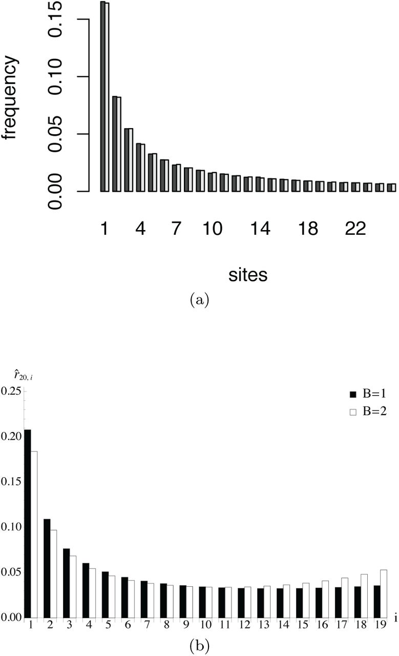
(a) Simulation and theoretical prediction for the neutral relative SFS and a uniformly distributed seed bank of length B = 10. For the simulation of the original discrete model the population size was chosen as 1000, we started without mutations and stopped the process after 400,000 generations to calculate the SFS as an average over 10,093 repetitions. The light gray bar shows the theoretical result, the dark gray bar shows the simulation outcome. In both cases a sample of 250 individuals was drawn. (b) Theoretical results for the relative SFS of a sample of size 20 are plotted for positive selection of strength σ = 2 without (B = 1) and with a seed bank of length B = 2.
As shown in Figure 2a, the neutral diffusion approximation is in line with the simulation results of the original discrete model. The theoretical relative SFS for a sample of 250 individuals approximates the simulated SFS, which is obtained as an average over 10,093 repetitions. In every iteration, the sample is drawn from an initially monomorphic population of 1000 individuals after 400,000generations(sothatthepopulationhas reached an equilibrium).Figure 2b illustrates the enhanced effect of selection proportional to the length of the seed bank.
3.2 Times to fixation
We assume that both y = 0 and y = 1 are absorbing states and start by considering the mean time until one of these states is reached in the diffusion process specified above. The mean absorption time  can be expressed as (Ewens 2004)
 where
where

For genic selection the integral in (9) cannot be analytically solved. For selective neutrality, we obtain  (see 359 e.g. Ewens 2004 for B = 1) by employing the drift term, the scale density and the probabilities of absorption as specified above.
Now, we evaluate the time until a mutant allele is fixed conditional on fixation as  , where
  . For genic selection the mean time to fixation in dependency of x can only be derived as a very lengthy expression in terms of exponential integral functions. The neutral result is found as
  and in accordance with a classical result (Kimura and Ohta 1969) for B = 1. For x → 0, we obtain
 where γ is Euler’s constant and Ei denotes the exponential integral function (Abramowitz and Stegun 1964).

(a) Simulation and theoretical prediction for the time to fixation of a seed bank model. The population size is 1000 and 50% of the individuals are initially of genotype A. We simulated 10,000 runs for each mean value. The simulated distribution of the time to fixation is shown in the histogram at the upper left corner taking the data of the simulated seed bank of length B = 12. (b) The ratios of the conditional fixation times with and without seedbank are plotted against the length of the seed bank B for neutrality and selection by employing (10). The additional index in the ratio is used to formally distinguish the cases with and without seed bank.
In Figure 3a, we compare the time to absorption of the original discrete seed bank model by means of simulations with the theoretical result obtained from the diffusion approximation. For bA we use uniform distributions, where we vary the expected values between 1 and 8 corresponding to the length of the seedbanksbetween1 and 15.We choose an initial fraction of 0.5 for the type-A genotypes. The simulations show a good agreement between our analytical approximation and the numerical simulations. In Figure 3b, we show the effect of the seed bank on the times to fixation conditional on fixation of the type-A genotype for neutrality and positive selection.
4. Discussion
Within this study, we develop a forward in time Fisher-Wright model of a deterministically large seed bank with drift occurring in the above-ground population. The time that seeds can spend in the bank is bounded and finite, as assumed to be realistic for many plant or invertebrate species. We demonstrate that scaling time in the diffusion process by a factor B2 generates the usual Fisher-Wright time scale of genetic drift with B being defined as the average amount of time that seeds spend in the bank. The conditional time to fixation of a neutral allele is slowed down by a factor B2 (Figure 3b, dotted line) compared to the absence of seed bank. These results are consistent with the backward in time coalescent model from Kaj et al (2001), and differs from the strong seed bank model of Blath et al (2015a). We evaluate the SFS based on our diffusion process and confirm agreement to the SFS obtained under discrete time Fisher-Wright simulations.
In the second part of the study, we introduce selection occurring at one of the two alleles, mimicking positive or negative selection. Two features of selection under seed banks are noticeable. First, selection is slower under longer seed banks (Figure 3b, solid line) confirming previous intuitive expectations (Hairston and Destasio 1988). Second, when computing the SFS with B = 2 and without seedbank(B = 1) under positive selection (σ = 2) we reveal a stronger signal of selection for the seed bank by means of an amplified uptick of high-frequency derived variants. This effect becomes more prominent with longer seed banks and also holds for purifying selection, under which an increase in low-frequency derived variants is induced by the seed bank. We explain this counterintuitive results as follows: longer seed banks increase, on the one hand, the selection coefficient σ generating a stronger signal at equilibrium (Figure 2b), and on the other hand, the time to reach this equilibrium state (Figure 3b). Our predictions are consistent with the inferred strengths of purifying selection in wild tomato species. Indeed, purifying selection at coding regions appears to be stronger in S. peruvianum than in its sister species S. chilense (Tellier et al 2011a) with S. peruvianum exhibiting a longer seed bank (Tellier et al 2011b).
Acknowledgements
This research is supported in part by Deutsche Forschungsgemein-schaft grants TE 809/1 (AT) and STE 325/14 from the Priority Program 1590 (DZ).
Appendix A Moran model with deterministic seed bank
We briefly sketch the arguments that allow to handle a Moran model with seed bank; the reasoning is completely parallel to the time-discrete case. In order to keep this appendix short, we do not take into account selection but focus on the neutral model.
A.1 Model
We start off with the individual based model. Let the population size be N, Xt the number of genotype-A-plants, µ the death rate, and b(s) the distribution of the ability for a seed at age s to germinate; we require  , and b(s) sufficiently smooth. Then,


Note that the delay process requires the knowledge of the complete history {Xs}s<t. The usual continuous limit for xt = Xt/N yields(with ε = 1/N)

If we rescale time in the usual way, τ = εt, and define  , we obtain

The aim here is to find heuristic arguments indicating that  approximates for ε → 0 the solution of a Moran diffusion process with rescaled time, paralleling equation (7).
Remark 2 In some sense, the terms in this time-continuous model are better to interpret than the parallel terms in the Fisher-Wright model: both terms within the brackets are moving averages, and clearly
 for a function uτ that is reasonably smooth. For the drift term, we find similarly

However, this bracket is divided by ε, and hence does not vanish for ε → 0. If we take a closer look, we find that a deviation of xτ from the moving average (the state of the seed bank) is punished. That is, the state of living plants can change only slower in comparison with a model without seed bank, and therefore for ε → 0 we expect a diffusion model at a 4slower time scale.
A.2 Scaling ε → 0
We drop the superscript ε in  , and write simply vτ. In order to use the arguments developed above, we discetize the stochastic differential-delay equation by the Euler-Maruyama formula, and find
 where ητ are i.i.d. N(0, 1) distributed, and the weights
  are chosen as

If we now define
 we may rewrite the discretized equation for vτ as
 where Lvτ = vτ−Δτ. We are now in the position of the proof for Prop. 4 (neglecting the time-dependency of β). As
 we have
 and conclude that approximately

Hence, for ε → 0 we expect (according to these heuristic arguments) that  satisfies the rescale diffusion equation

If we define G = 1/μ, the average inter-generation time of living plants, this equation becomes even more close to that derived for the Fisher-Wright case,
 as it becomes clear that the correction factor 1 + B/G measures the average time a seed rests in the soil in terms of generations.


