

Abstract
Despite being heritable and under selection, traits often do not appear to evolve as predicted by evolutionary theory. Indeed, conclusive evidence for contemporary adaptive evolution remains elusive in wild vertebrate populations, and stasis seems to be the norm. Here we show that a wild rodent population has evolved to become lighter, but that both this evolutionary change and the selective pressure that drives it are not apparent on the phenotypic level. Thereby we demonstrate that understanding and predicting the response of wild populations to environmental change requires an explicitly (quantitative) genetic approach, and that natural populations can show a rapid and adaptive, but easily missed, evolutionary response.
Given the rapid anthropogenic environmental change experienced by populations around the world, there is an increasing need for the ability to predict the evolutionary dynamics of wild populations 1. However, predictive models of evolution have so far largely failed when applied to data from wild populations. For example, natural and sexual selection almost universally favour larger individuals 2, and body size is typically highly heritable 3 ,4. Nevertheless, while species tend to get larger over geological timescales 5 ,6, conclusive evidence for a contemporary evolutionary response to selection remains elusive for wild animal populations—for body size 7 or any other fitness-related quantitative trait for that matter 8 ,9. This mismatch between the predicted and the observed response, also referred to as the ‘stasis paradox’ 8, and our inability to predict the evolutionary dynamics of wild populations in general, is a major concern that is in urgent need of a resolution.
Although studies that find a discrepancy between the observed and predicted rate of evolution are plentiful, they typically have two limitations: First, their predictions rely on the breeder’s equation, which assumes that phenotypic selection, quantified as the covariance between a trait and relative fitness, is causal 10; Second, they compare this prediction either to the trend in mean phenotype over time 8, or to flawed estimates of genetic change based on estimated breeding values 11, 12. Here we instead apply a comprehensive analytical framework to long-term individual-based data from a wild rodent population, in order to directly quantify selection and evolution of body mass. This allows us to compare the observed genetic change to a range of evolutionary predictions, and to unravel the causes underlying the stasis paradox.
Results
Based on nine years of data on an alpine population of snow voles 13, 14 (Chionomys nivalis, Martin 1842), we find that relatively heavy individuals both survive better (p = 0.04) and produce more offspring (p = 0.003). This generates strong phenotypic selection favouring heavier individuals (selection differential S = 0.86 g, p < 10−5). In line with other morphological traits 3 ,4, variation in body mass has a significant additive genetic component (VA=4.34 g2, 95%CI [2.40;7.36]), which corresponds to a heritability (h2) of 0.21. Similarly, we find significant additive genetic variance in fitness (VA=0.10; 95%CI [0.06;0.19], h2 = 0.06), measured as relative lifetime reproductive success (rLRS).
Given the observed heritability and selection differential (S), the breeder’s equation (R = h2S) predicts an adaptive evolutionary response (R) in body mass 10, 15, i.e. an increase in the mean breeding value for body mass over time, of 0.22 g/year (Fig 2A UBE). However, over the past nine years (approximately eight generations), mean body mass has increased at a 8.8-fold higher rate (1.95 g/year; 95%CI [1.61;2.28]; p< 0.001). This increase is however mostly mediated by a change in the demographic structure (Fig. S1), and correcting for this change reveals a systematic trend in mass that is not significant and small at best (0.08 g/y; 95%CI [-0.02;0.18]; p=0.14) (Fig. 1A & Fig. 2A PT). This mismatch between the predicted evolutionary change based on the breeder’s equation and the change observed provides yet another example of the stasis paradox 8.

(A): Year-specific mean mass corrected for age, sex and date of measurement, with 95%CI. (B): Cohort-specific mean estimated breeding value for mass with their 95%CI and the trend in breeding value with 95%CI.

(A): Rates of evolutionary change predicted by (from left to right) the breeder’s equation in its multivariate form (MBE), the multivariate breeder’s equation while constraining the genetic correlations to zero (MBEp=0), and the univariate breeder’s equation (UBE), followed by the phenotypic trend (PT), the trend in predicted breeding values (TPBV) and the genetic change estimated by the Price equation (GCPE). (B): Phenotypic, genetic and environmental selection differential for total selection (LRS), fertility selection in males (ARS♂) and females (ARS♀), viability selection in juveniles (ϕJuv) and in adults (ϕA). Both panels show posterior modes, with vertical lines indicating 95%CI.
In an attempt to resolve this paradox, several explanations have been put forward. For example, it has been suggested that the predicted positive genetic trend, i.e. an increase in breeding values, is being masked by an opposing phenotypically plastic response 8, 16. Interestingly however, if we test for a trend in the best linear unbiased predictors (BLUPs) of breeding values for mass, while taking into account their non-independence and sampling variance 11, 12, we find that predicted breeding values have declined rather than increased over the past nine years (-0.07 g/year, pMCMC=0.06; Fig. 1B & Fig. 2A TPBV), and this despite the BLUPs approach underestimating rates of evolution if genetic and phenotypic changes go in opposite directions 11.
To corroborate this, at first sight maladaptive, genetic trend, and to obtain insight into its origin, we directly estimated the additive genetic covariance between mass and fitness, which, based on the Robertson-Price’s equation, provides an unbiased estimate of the rate of genetic change per generation 10, 17, 18. As expected from the negative trend in the BLUPs of body mass breeding values, this estimate of genetic change in mass is strongly negative and highly significant (pMCMC < 0.001; Fig. 2A GCPE), and when normalized by a mean generation time of 1.2 years, provides a rate of evolutionary change of -0.29 g/year (95%CI [-0.55; -0.07]). Importantly, this amount of change is unlikely to have happened solely through genetic drift (pMCMC < 0.001; Fig. S2) 12, and therefore most likely reflects a response to selection favouring genetically lighter individuals. However, why is evolution taking place in a direction that is opposite to phenotypic selection?
The negative genetic covariance between mass and fitness may be the result of selection acting upon one or more traits positively correlated with mass on the phenotypic level, but negatively on the genetic level (Fig. 3) 19, 20. However, the genetic correlations among the three morphological traits for which we have data—body mass (m), body length (b) and tail length (t)—are all positive (estimates and 95%CI: ρm,b = 0.79 [0.06; 0.93]; ρm,t = 0.40 [0.01; 0.66]; ρt,b = 0.56 [−0.04; 0.85]), and the predicted response based on the multivariate breeder’s equation (Fig. 2A MBE) is very similar to that based on its univariate counterpart (Fig. 2A UBE), as well as to that based on a multivariate breeder’s equation constraining the correlations to zero (Fig. 2A MBEρ=0). So, although we cannot exclude that selection on other, unmeasured, traits does indirectly shape body mass evolution, there is no evidence for genetic correlations generating the striking mismatch between observed and predicted genetic change.

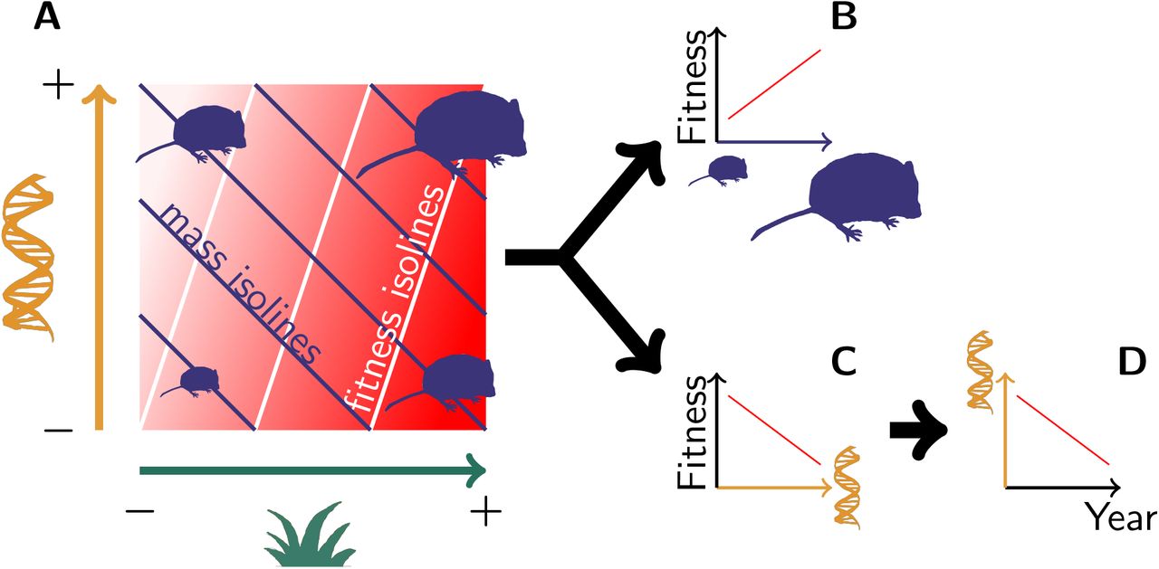
(A) Both genetic variation (orange) and environmental variation (green) contribute to mass variation, but their respective effect on fitness (the redder the fitter) is not equivalent. This pattern leads to (B) a phenotypic selection for heavier voles, along with (C) a “genetic selection” for lighter genotypes, thus leading to (D) an evolution towards lighter voles.
Instead, we have strong evidence for the positive association between mass and fitness being mediated solely by a covariance among their environmental components 10, 21, 22. The phenotypic selection differential (σP(m,ω)) is equal to the sum of the additive genetic and environmental selection differentials for mass (σA(m,ω) and σE(m,ω), respectively) 10, 17, 18, and from this it follows that because σP(m,ω) is positive while σA(m,ω) is negative, the environmental covariance is large and positive (Fig 2B LRS). In other words, while environmental conditions that make voles heavy also make them successful at reproducing and surviving, there is no causal positive relationship between breeding values for mass and fitness. The assumption that selection is blind with respect to whether phenotypic variation is genetic or environmental in origin (i.e. σA(m,ω)/(σA(m,ω) + σE(m,ω)) = h2), which is central to evolutionary predictions based on the breeder’s equation, is thus violated.
The question that remains is what generates the negative genetic selection on mass, and given that selection acts on phenotypes rather than genotypes, why this is not reflected in the direction of phenotypic selection. In search of the subject of negative selection, we therefore computed sex-and age-specific genetic covariances between mass and fitness components, allowing us to identify what fitness component is negatively associated with genes for being heavy.
Whereas the genetic covariances between mass and both relative annual reproductive success and adult survival are close to zero in both sexes (Fig. 2B), the genetic covariance between mass and over-winter survival probability is negative in juveniles (-0.98 [-2.44;-0.18] on a logit scale, pMCMC=0.01). Because the genetic correlation between juvenile and adult mass is positive (rA = 0.88; 95%CI [0.39;1]) and significantly different from 0 (p=0.004), but not from 1 (p=0.35), selection on juvenile mass can shape genetic variance for mass at all ages, and thereby contribute to the observed negative genetic change 23. While this shows that negative viability selection of juvenile mass is responsible for the genetic change toward smaller individuals, how come survival is higher for heavier phenotypes and lighter genotypes?
Juvenile mass covaries positively with both within-and between-year survival (p = 0.009 and p =1.3 x 10⁻⁶, respectively). However, juveniles can only be captured when they first leave their burrow, at an age of approximately three weeks 24 and a weight of 12 to 20 g, and they may continue to be captured until the end of the season, when they can reach weights of up to 50 g. Because of growth, mass measurements are therefore not directly comparable among juvenile individuals. Indeed, at least part of the positive phenotypic selection on juvenile mass is likely to be mediated by age-related variation in both mass and in the probability of survival to the next year 25. In addition, viability selection introduces non-random missing data, which results in biased estimates of viability selection on mass 25, 26. However, this doesn’t mean that some heritable aspect of the growth curve is not negatively selected 21, 23, 25.
We used a Bayesian model to simultaneously infer juvenile growth curves and birth dates for all juveniles observed at least once, irrespective of when and how often they have been captured. Although we cannot account for viability selection acting before the first capture, this enabled us to quantify viability selection on asymptotic juvenile mass—the adult mass as estimated from the growth curve—, and thereby compare all individuals at the same developmental stage, irrespective of their fate. This provides an estimate of viability selection that is unbiased by growth and non-random missing data due to mass-dependent mortality occurring after the first capture.
Snow fallen during the preceding winter is a major ecological factor constraining the onset of reproduction in spring, with reproduction starting on average 40 days after the snow has melted (SE 4.5, p =4 x 10⁻⁵) (Fig. 4A). Therefore, juveniles only have a limited amount of time to grow and reach their adult mass before the return of winter. Assuming little variation in growth rates, juveniles with a smaller potential mass will be closer to their adult mass at the beginning of winter and will survive better (Fig. 4D). In line with this, while selection on asymptotic mass was slightly negative when averaged over all years and the complete snow-free season (pMCMC=0.13), it interacted significantly with the number of days between birth and the first snowfall of that year (pMCMC=0.008), with individuals born closer to the first snow fall being more strongly selected for a small asymptotic mass. The mechanism underlying this pattern is unknown, but could be related to trade-offs between growth and vital physiological processes 27, 28.

(A): Births (black dots) only occur during the snow free season (snow depth in blue), (B): which in 2008-2014 has been shorter than in the preceding 8 year. Therefore, (C) despite a positive phenotypic selection on body mass (blue), asymptotic mass was selectively neutral in 2006-2007 (brown), and was negatively selected in 2008-2014 (red), as a result of (D) the selective disappearance of heavy individuals that were born too close to the onset of winter (blue vertical line) during 2008-2014.
Based on our model, in 2006 and 2007, when the snow-free period was long (Fig. 4B), most juveniles reached their asymptotic mass and there was no selection on asymptotic mass (Fig. 4C; D; S3). However, in all subsequent years, the snow-free period was much shorter, and there was selection for a smaller asymptotic mass, with 2008 being the most extreme year (Fig. 4C). Interestingly, the length of the snow-free period in the years 2008 to 2014 has been significantly shorter than during the preceding six years (Fig. 4B), suggesting that the shortening of the snow-free season, and thereby selection for smaller asymptotic mass, is a novel phenomenon that the population is currently in the process of adapting to. Indeed, although model complexity and data availability prohibit disentangling genetic and environmental sources of variation in asymptotic mass among individuals and over time, the cohort born in 2013 had an asymptotic mass that was 1.02 g smaller than the cohort born in 2006 (p=0.049). This decrease is predicted to increase population-level juvenile survival by 2.5% and is therefore adaptive.
On the whole, we have shown that while cases of evolutionary stasis appear to be commonplace, these may be attributable to overly simplistic predictions of evolutionary change based on estimates of phenotypic selection that fail to account for 1) a disproportional environmental co-variance between trait and fitness, and 2) non-random missing data whenever viability selection acts during ontogeny. Therefore, the quantification, and most importantly, the prediction of evolution in the wild requires the direct estimation of more complex patterns of inheritance, genetic correlations and selective pressures.
Methods
Snow vole monitoring. Monitoring of the snow vole population began in 2006 and the present work uses data collected until fall 2014. The study site is located at around 2030m above sea level, in the central eastern Alps near Churwalden, Switzerland (46°48’ N, 9°34’ E). It consists of scree, interspersed with patches of alpine meadows and surrounded by habitat unsuitable for snow voles: a spruce forest to the West, a cliff to the East and large meadows to the North and South. The species is considered a rock-dwelling specialist 24, and accordingly at our study site it is almost never captured outside of the rocky area. This means that it is easy to monitor the whole population, and that the population is ecologically fairly isolated. Trapping throughout the whole study area took place during the snow-free period, between late May and mid-October, and was repeated for two (in one year), three (in three years) or five (in five years) sessions of four trapping nights each. All newly-captured individuals weighing more than 14 g are marked with a subcutaneous passive transponder (PIT, ISO transponder, Tierchip Dasmann, Tecklenburg). Additionally, an ear tissue sample was taken (maximum 2 mm in diameter) using a thumb type punch (Harvard Apparatus) and stored in 100% ethanol at −20°C. DNA extracted from these samples was genotyped for 18 autosomal microsatellites developed for this population 29, as well as for the Sry locus to confirm the sex of all individuals. Finally, another Y-linked marker as well as a mitochondrial marker were used check for errors in the inferred pedigree (see below). An identity analysis in CERVUS v.3.030 allowed us to identify animals sampled multiply, either because they lost their PIT, or because at their first capture as a juvenile they were too small to receive a PIT. All the analyses were carried out in R 31, using various packages mentioned thereafter.
Pedigree inference. Parentage was inferred by simultaneously reconstructing paternity, maternity and sibship using a maximum likelihood model in MasterBayes 32. Parentage was assigned using a parental pool of all adults present in the examined year and the previous year, assuming polygamy and a uniform genotyping error rate of 0.5% for all 18 loci. As it is known that in rare cases females reach sexual maturity in their year of birth 24, we matched the genotypes of all individuals against the genotypes that can be produced by all possible pairs of males and females. We retrieved the combinations having two or less mismatches (out of 18 loci) and ensured that parental links were not circular and were consistent time-wise. This way, we identified eight young females as mothers of animals born in the same year, with a known father but a mother not yet identified. All of these females were relatively heavy (>33 g) at the end of the season and their home-ranges matched those of their putative offspring. Excluding these parental links had however effect on the estimation of quantitative genetic parameters. Finally, the pedigree was checked using a polymorphic Y-linked locus developed for this population 33, as well as a fragment of the mitochondrial DNA control region, amplified using vole specific primers 34. There were no inconsistencies between the transmission of these three markers and the reconstructed pedigree. The final pedigree had a maximum depth of 11 generations and a mean of 3.8 generations. It consisted of 987 individuals with 458 full sibship, 3010 half sibship, 764 known maternities and 776 known paternities, so that, excluding the base population, 86% of the total parental links were recovered.
Traits. The recapture probability from one trapping session to the next was estimated to be 0.924 (SE 0.012) for adults and 0.814 (SE 0.030) for juveniles using mark-recapture models. Thus, with three trapping session a year, the probability not to trap an individual present in a given year is below 10−3. Not surprisingly, no animal was captured in year y, not captured in y + 1, but captured or found to be a parent of a juvenile in y + 2 or later. Therefore, capture data almost perfectly matches over-winter survival. However, as is almost always the case in these type of studies, we are unable to separate death from from permanent emigration. Importantly however, as both have the same consequences on the population level, this does not affect our estimates of selection.
Annual and lifetime reproductive success (ARS and LRS, respectively) were defined as the number of offspring attributed to an individual in the pedigree, either over a specific year or over its lifetime. 56 individuals born of local parents were not captured in their first year, but only as adult during the next summer, probably because they were born late in the season and we had only few opportunities to catch them. This means that we miss a fraction of the juveniles that are not observed in their first year and die, or emigrate, during the following winter. We acknowledge that our measures of ARS and LRS partly conflate adult reproductive success and the viability of those juveniles that were born late in the season, but our measures are the most complete measures of reproductive success available in this system.
We used relative LRS (ω) as proxy for fitness 19, where  . Here, Ns,t is the number of individuals of same sex as the focal individual i, present in the cohort t, so that
  is the sex-specific, cohort-specific mean of LRS. The latter is required as the mean LRS differs between males and females due to imperfect sampling 10. In addition, we used cohort-specific means in order to account for variations in population size.
Generation time was defined as the mean age of parents at birth of their offspring 35.
Mass (m) was measured to the nearest gram with a spring scale. Both body length (b), measured from the tip of the nose to the base of the tail, and tail length, measured from the tip to the base of the tail (c), were measured to the closest mm with a calliper while holding the animal by the tail.
Selection. Selection differentials were estimated using bivariate linear mixed models, as the individual-level covariance between fitness and mass (corrected for sex, age and cohort). However, while this provides the best estimate of the change in trait mean due to selection 19, because the distribution of fitness is not Gaussian, it cannot be used to estimate confidence intervals. Hence, the statistical significance of selection was tested using a univariate over-dispersed Poisson generalized linear mixed model (GLMM) in which LRS was modelled as a function of individual standardized mass (corrected for sex, age and cohort). Note that the latter estimates the effect of mass on a transformed scale, and therefore cannot be directly used to quantify an effect of selection on the original scale measured in grams 36. The significance drawn on the basis of the GLMM was confirmed by non-parametric bootstrapping.
Similarly, we tested for the significance of selection through ARS only, using an over-dispersed Poisson GLMM including sex as a fixed effect, and year and individual as random effects. Here, modelling capture probability does not help to model survival because the year-to-year individual recapture probability is virtually 1. Therefore, selection on year-to-year survival was tested for by a binomial GLMM. This model included sex, age and their interaction as fixed effects, and year as a random effect.
Quantitative genetic analyses. We used uni-and multivariate animal models to estimate additive genetic variances, covariances and breeding values 15, 37, 38 with MCMCglmm 39. All estimations were carried out in a Bayesian framework in order to propagate uncertainty when computing composite statistics such as heritabilities and rates of genetic change 40. All estimates provided in the text are posterior modes and credibility intervals are highest probability density intervals at the level 95%. All the animal models were run for 1,300,000 iterations with a burnin of 300,000 and a thinning of 1,000, so that the autocorrelations of each parameter chain was less than 0.1. Convergence was checked graphically and by running each model twice.
Univariate models: We first carried out univariate model selection, fitting models without an additive genetic effect, to determine which fixed and random effects to include. Based on AICc 41, and fitting the models by Maximum of Likelihood in lme4 42, we obtained a model that predicts the mass mi,t of individual i at time t by: age, as a factor (juvenile or adult); sex as a factor; the interaction between age and sex; Julian dates and squared Julian dates, which were centered and divided by their standard errors in order to facilitate convergence; the interaction between age and Julian date; the interaction between sex and Julian date; the three way interaction between age, sex and Julian dates; a random intercept for individual; and a random intercept for year. The inclusion of year accounts for non-independence of observation within years, while individual accounted for multiple measurements 43. We then fitted an animal model by adding a random intercept modelling variance associated with mother identity 38, and a random intercept modelling additive genetic variance. Although it was not included in the best models, we kept inbreeding coefficient as a covariate, because leaving it out could bias the later estimation of additive genetic variation 44. Nevertheless, animal models fitted without this covariate gave indistinguishable estimates.
Multivariate models: Univariate animal models can be expanded to multivariate models in order to estimate genetic correlations, genetic gradients and genetic differentials.

Here X, D1, D2, D3 and D4 are design matrices relating observations to the parameters to estimate, b is a matrix of fixed effects, a, m, p and y are random effects accounting for the variance associated with breeding value, mother, permanent environment and year, respectively. The fixed part of the model matches that used for each trait in univariate models.
The most important aspect of this model is that a, the matrix of breeding values, follows a multivariate normal distribution:
 where A is the relatedness matrix between all individuals, and G is the G-matrix, i.e. the additive genetic variance covariance matrix between all traits.

For any trait z, σA(z,ω) is the genetic differential, that is, the rate of evolutionary change according to Price equation 10. For mass, the genetic differential was also estimated using a bi-variate animal model, of mass and fitness, in order to confirm the value of this crucial parameter. For two traits z and y, the genetic correlation is  . The vector of selection differentials on the three traits (S) was estimated as the sum of the vectors of covariances between traits and w in the variance-covariance matrices for a, p and r; which was equivalent to the selection differential computed in the paragraph on selection above. Let G’ be a subset of G excluding the column and the row that contain w. The vector of selection gradients on the three traits (β) was estimated as (G’ + P’ + R’)−1S, where P’ and R’ are the equivalent of G’ for permanent environment effects and for residuals, respectively.
The prediction of the multivariate breeders equation is obtained by  , while the multivariate breeders equation ignoring genetic correlations is obtained by multiplying the G’ matrix by the identity matrix 20:
  .
.
Test of genetic correlations: We used ASReml-R 45, 46 to test the genetic correlation between mass in adults and in juveniles against 1 and 0, by considering them as two separate traits. We first ran an unconstrained model and then reran it with the genetic correlation parameter set to 0.99 (and not exactly to 1 because ASReml cannot invert matrices with perfect correlations), or 0 respectively. The fit of the unconstrained model was then compared to that of the two constrained models using a likelihood ratio test with one degree of freedom 47.
Birth date and growth prediction. Using the Bayesian programming environment JAGS 48, we fitted a multivariate Bayesian model to mass measurements of the 613 juveniles with mass data, and to their overwinter survival. The model simultaneously estimated individual growth curves—that is birth dates, individual growth rates and asymptotic masses of all juveniles—and the effect of asymptotic mass on overwinter survival. The model clustered juveniles from the same mother born in the same year into litters, using a mixture of birth dates depending on litter affiliations (see e.g. 49 for a similar approach), assuming a maximum of five litters per year and assuming that successive litters are at least 20 days apart 24. The birth weight was assumed not to vary among individuals. Preliminary model selection assuming no differences in asymptotic masses among individuals selected a monomolecular growth model (ΔDIC > 80) over Gompertz and logistic models, as defined in 50. The model accounted for measurement error in mass, assuming that the standard deviation of the errors was that observed in animals measured multiple time on the same day (2.05g). Within the model we performed a logistic regression of year-to-year survival on sex and asymptotic mass, in order to estimate the overall viability selection on asymptotic mass. We ran the full model again, adding time until the first snow fall and its interaction with asymptotic mass in the logistic regression, in order to test for the effect of the length of snow free period on the selection on asymptotic mass. We use the estimates of these two models to predict the survival probability as a function of asymptotic mass for every year, or for groups of years, depending on the distribution of birth dates and on the timing of the first snow fall. Three MCMC chains were run for 6,300,000 iterations, with a burnin of 300,000 and a thinning of 6,000. Convergence was assessed by visual examination of the traces, and by checking that the  . Convergence was not achieved for the litter affiliations of 25 individuals as well as for one asymptotic mass, thus generating a bit more uncertainty in the estimations. The fit of the model was assessed using posterior predictive checks on the predictions of individual masses (p=0.46) and survival probabilities (p=0.49). The JAGS code for this model can be found at https://github.com/timotheenivalis/SelRepSel.
Author Contributions
T.B. designed and conducted the analyses. P.W. and G.C. initiated the monitoring, and developed methods for genotyping and pedigree inference. E.P. led the monitoring and conceived the study. T.B. and E.P. wrote the manuscript.
Acknowledgements
Thanks to all those who helped out in the field. Thanks to Wolf U. Blanckenhorn, Jarrod D. Hadfield, Lukas F. Keller, Marc Kéry, Hanna Kokko, Chelsea J. Little, Pirmin Nietlisbach, Barbara Tschirren and Ashley E. Latimer for comments and discussions. Weather data were provided by MeteoSwiss. The snow vole monitoring was authorised by the Amt für Lebensmittelsicherheit und Tiergesundheit, Chur, Switzerland. T.B. is funded by a Swiss National Science Foundation project grant (31003A_141110) awarded to EP. The data reported in this paper are archived at…Dryad The authors declare no conflict of interest. T.B. designed and conducted the analyses. P.W. and G.C. initiated the monitoring, and developed methods for genotyping and pedigree inference. E.P. led the monitoring and conceived the study. T.B. and E.P. wrote the manuscript.
References


