

SUMMARY
Like many other species, the plant Arabidopsis thaliana has been introduced in recent history from its native Eurasian range to North America, with many individuals belonging to a single lineage. We have sequenced 100 genomes of present-day and herbarium specimens from this lineage, covering the time span from 1863 to 2006. Within-lineage recombination was nearly absent, greatly simplifying the genetic analysis, allowing direct estimation of the mutation rate and an introduction date in the early-17th century. The comparison of substitution rates at different sites throughout the genome reveals that genetic drift predominates, but that purifying selection in this rapidly expanding population is nevertheless evident even over short historical time scales. Furthermore, an association analysis identifies new mutations affecting root development, a trait important for adaptation in the wild. Our work illustrates how mutation and selection rates can be observed directly by combining modern genetic methods and historic samples.
HIGHLIGHTS
A historically young colonizing lineage of Arabidopsis thaliana allows observation of contemporary evolutionary forces.
Genomes from specimens collected over 150 years support direct calculation of mutation rates occurring in nature.
Drift predominates, but purifying selection is evident genome-wide over historical time scales.
New mutations with phenotypic effects can be identified and traced back in time and space.
INTRODUCTION
If we want to understand evolution and especially adaptation, we need to know rates of mutation and selection, which together determine the substitutions that can be observed in a population. Typically, one tries to infer evolutionary parameters from patterns of genetic diversity in extant individuals of a species. Unfortunately, demographic and genetic factors such as migration, fluctuating population sizes, recombination and gene conversion greatly complicate such inferences. Many scientists have therefore chosen to focus on mutations only, measuring their accumulation in artificial conditions, using mutation accumulation lines grown in the laboratory (Halligan and Keightley, 2009), or over very short time scales, for example in human parent-offspring trios (Roach et al., 2010).
An alternative approach is the use of older, but still simple lineages with limited genetic diversity, such as colonizing populations that have undergone a recent, strong genetic bottleneck. Such populations can be considered natural experiments in which one can test ecological or evolutionary hypotheses (Gauze, 1934; Maron et al., 2004; Sax et al., 2007). Recent colonization events permit the quantification of evolutionary forces related to adaptation – mutation, selection, genetic drift, recombination – that are still not well understood in invasion ecology (Barrett, 2014; Bock et al., 2015; Lee, 2002).
Humans have increasingly blurred biogeographical boundaries of species outside their native range by planned or serendipitous dissemination. While the exact reasons for success or failure in alien environments remain unclear, many species can become established in new areas, with North America being the continent with the highest number of naturalized plants (van Kleunen et al., 2015). Among these is the model plant Arabidopsis thaliana, which is native to Eurasia but has recently colonized and spread throughout much of North America (Platt et al., 2010). Although A. thaliana is not an invasive species, it has traits typical for successful colonizers, such as a high selfing rate, a durable seed bank and a short generation time (Baker, 1965).
Colonizing populations often start with very few individuals and therefore have low genetic diversity. The N. American A. thaliana population is much less diverse than what is seen in the native range, with one predominant lineage, named haplogroup-1 (HPGI), accounting for about half of all N. American individuals (Platt et al., 2010). The success of an isolated, selfing lineage that is genetically very uniform seems to contradict the common idea that such lineages are evolutionary dead-ends because they can adapt only through de novo mutations, a process predicted to be much slower than adaptation from standing variation (Barrett and Schluter, 2008), although we cannot know how long this lineage will last.
Ideally, to evaluate all evolutionary trajectories, including unsuccessful ones, one should have access not only to the evolved extant individuals, but also to their “unevolved” ancestors. The power of temporal transects has been aptly demonstrated with the genetic analysis of historical and archaeological samples of humans and microbes, relying on advances in the study of ancient DNA (aDNA) (Orlando et al., 2015; Shapiro and Hofreiter, 2014). Natural history collections that cover the past several hundreds of years offer an exciting, underused resource for such studies (Martin et al., 2013; Staats et al., 2013; Vandepitte et al., 2014; Weiß et al., 2015; Yoshida et al., 2013).
There is a rich history of sampling plants and storing them in herbaria. Importantly, herbaria do not merely house exotic, rare species collected in the more distant past, but also common plants that have been sampled for many decades over and over again, making them powerful tools for monitoring recent colonization events in space and time (Crawford and Hoagland, 2009; Lankaua et al., 2009). Such a resource exists for N. American A. thaliana. Here, we compare genomes from herbarium specimens, collected between 1863 to 1993, and from live individuals, collected between 1993 and 2006, to date the origin of this lineage, and infer mutation rates, selection, demography and migration routes. We also identify de novo mutations in this lineage that are associated with phenotypes likely to be under selection in the wild, which in turn correlate with climatic variables. Our analyses of a colonizing A. thaliana lineage serve as a blueprint for future studies of similar colonizing or otherwise recently bottlenecked populations, in order to understand mutation, selection and rapid adaptation in nature.
RESULTS AND DISCUSSION
Herbarium and modern HPGI genomes
When analyzed with 149 genome-wide, intermediate-frequency SNP markers, about half of over 2,000 North American A. thaliana individuals collected between 1993 and 2006 were found to be very similar (Platt et al., 2010). A recent study of 13 individuals from this collection confirmed that their genomes were indeed almost identical (Hagmann et al., 2015). We selected 74 additional individuals for illumina whole-genome sequencing, aiming for broad geographic representation, and, where available, at least two accessions per collection site (Fig. 1; Table S1).
Latitude and longitude for historic samples were imputed from the geographic centroid of the most accurate toponym described in the herbarium specimen label.
Key of abbreviations of herbarium collections or seed sources:
UCONN = University of Connecticut herbarium; CFM = Chicago Field Museum; NY = New York Botanical Garden; ABRC = Arabidopsis Biological Resources Center; OSU = Ohio State University H* indicate herbarium samples that cluster with the modern HPGI clade rather than the historic HPGI clade in Fig. 3.
Geographic location highlighted in Fig. 1.

(A) Sampling location of herbarium specimens (blue) and modern individuals (green). (B) Temporal distribution of samples (randomly Jittered in a y axis for visualization). Stars indicate four herbarium accessions that nest in the clade of modern accessions. See Fig. 3.
See also Figure S1.
We aimed to complement these data with genome information from 36 herbarium specimens collected between 1863 and 1996 (Fig. 1; Table S1). To avoid contamination from exogenous sources, DNA extraction and illumina library preparation were carried out in a clean-room facility. Between 30% and 86% of sequencing reads mapped to the A. thaliana reference genome (Fig. S1A), compared to ∼90% for the modern individuals. A number of biochemical features define aDNA and can be used to verify authenticity (Krause et al., 2010; Prüfer and Meyer, 2015; Weiss et al., 2015). Typical for aDNA, most DNA fragments were shorter than 100 bp (Fig. S1B). Deamination of cytosines to uracils at the end of aDNA fragments (Hofreiter et al., 2001) is seen as cytosine to thymine (C-to-T) substitutions upon sequencing (Briggs et al., 2007), and this rate of substitution at first sequenced base was between 1.3 to 4.4% in the different sequenced libraries (Fig. S1C). Moreover, aDNA breaks preferentially at purines (Briggs et al., 2007), and purines were 1.5 – 1.8-fold enriched at fragment ends (Fig. S1D). Together this indicated that DNA recovered from A. thaliana herbarium specimens was authentic.
Coverage of sequenced historic samples was 3-to 42-fold for herbarium and 22-to 105-fold for modern samples. To identify within-lineage sequence differences, reads were mapped against an HPGI pseudoreference (Hagmann et al., 2015). We focused on single nucleotide polymorphisms (SNPs) because accurate identification of structural variants from short reads is difficult, particularly so in old DNA molecules that have suffered from chemical breakage (Weiß et al., 2015). The herbarium genomes subsequently confirmed as HPGI had 96.8 to 107.2 Mb of the HPGI pseudoreference covered by at least three reads, compared with 108.0 to 108.3 Mb in the modern genomes. We found 109 to 222 SNPs relative to the HPGI pseudoreference in the herbarium genomes, and 186 to 299 SNPs in the modern genomes.
Diversity and relationships within HPGI
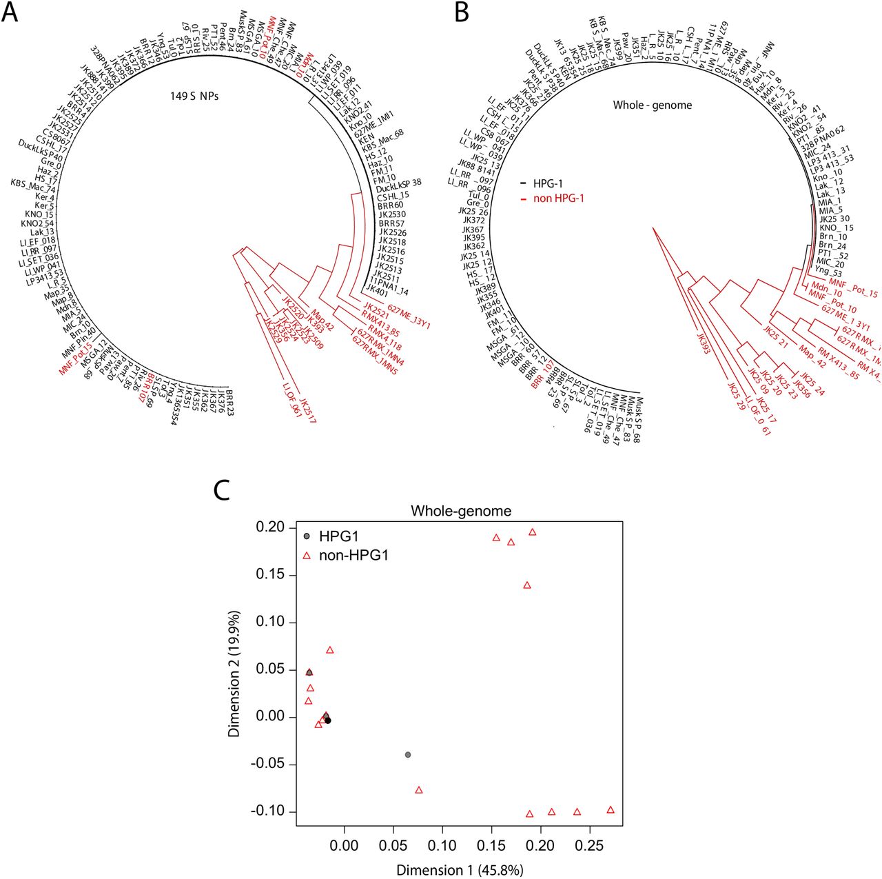
Among the 87 modern individuals, seven clearly did not belong to the HPGI lineage, which could be due to errors in the initial genotyping, or to lack of resolution based only on 149 SNPs. Four additional individuals that were identical to the rest of the HPGI lineage at the 149 genotyped SNPs (Fig. S2A) appeared to have small stretches of introgression from other lineages and were therefore classified as non-HPGI, as indicated by several methods (e.g., Fig. S2B). Of the 36 herbarium samples, nine turned out to be non-HPGI lines (Fig. S2A and S2B). In total, 76 modern and 27 herbarium samples were identified as HPGI by means of neighbor-joining trees and multidimensional scaling (MDS), including the 12 oldest herbarium specimens (Fig. S2C). The obvious homogeneity and abundance of HPGI compared to other N. American lineages greatly simplified its classification.
After removal of non-HPGI lines, the HPGI neighbor-joining tree reconstruction resulted in a star-like phylogeny (Fig. 2A). MDS could not differentiate samples within the HPGI group, with the first and second dimensions each explaining only small amounts of variance, 8.8% and 8.0% (Fig. 2B). A parsimony network identified a small fraction of reticulations indicative of intra-HPGI recombination (Fig. 2C). Removing three potential intra-HPGI recombinants resolved the reticulations (Fig. 2D). The remaining 73 modern and 27 herbarium samples (Table S1) appeared to constitute a clonal lineage devoid of effective recombination and population structure, with no SNPs detected in chloroplasts nor mitochondrial genomes, and with very low genome-wide nuclear diversity (π = 0.000002, θw = 0.00001, 4,368 segregating sites), which is two orders of magnitude lower than in the native range (θw = 0.008) (Cao et al., 2011; Nordborg et al., 2005). The enrichment of low frequency variants (Tajima’s D = −2.84) and low levels of polymorphism in surveyed genomes is consistent with a recent bottleneck followed by population expansion. We hypothesize that the bottleneck corresponds to a colonization founder event, likely by one or only few very closely related individuals.

(A) Neighbor-joining tree. Consensus of 1,000 bootstrap replicates. Branch lengths indicate number of base substitutions. (B) First two dimensions of a multidimensional scaling plot based on pairwise identity-by-state distances. Fraction of variance explained given in parentheses. Phylogenetic network of all samples using the parsimony splits algorithm, before (C) and after (D) removing intra-HPGI recombinants.
See also Figure S2.
Although there was little evidence for intra-lineage recombination among the 100 remaining individuals, a few isolated SNPs were shared between independent branches of the tree (Fig. 2A). We therefore also formally estimated recombination within HPGI. The estimate was much lower (4Ner = ρ = 3.0 × 10⁻⁶ cM bp−1) than for a similar-sized collection of diverse A. thaliana individuals from the native range (ρ = 7.5 × 10⁻² cM bp−1) (Choi et al., 2013). Linkage disequilibrium parameter D’ did not decay with physical distance (intercept = 0.99, slope = 0.00, p < 0.0001) among all SNP pairs. Furthermore, only 0.02% of SNP pairs were not in complete linkage disequilibrium (D’<l), indicating extensive linkage between chromosomes. The four-gamete test, which determines whether all four possible gametes (ab, aB, Ab, AB) are observed for two segregating loci, revealed that all configurations of SNPs could be explained with as few as 38 recombination events for the 100 genomes. We argue that this number of potential recombination events is sufficiently small that it does not invalidate the application of phylogenetic methods to the HPGI genomes, even though such methods are normally not appropriate for genome-wide analyses. Indeed, other sources of failure of the four-gamete test and the violation of phylogenetic assumptions could be sequencing errors, or lineage sorting of segregating sites from the ancestral population.
To describe intra-HPGI relationships in a more sophisticated manner than with a simple neighbor-joining approach, we used Bayesian phylogenetic inference. We took advantage of the broad distribution of collection dates of our herbarium samples (Fig. 1B) for tip calibration of phylogenetic trees. The method that we used reconstructs a tree calibrated in time, based on genetic distance between samples collected at different points in time. In this tree, the 76 modern individuals formed a virtually monophyletic clade, with only four interspersed herbarium samples from the second half of the 20th century (Fig. 3A, B, Table S1). Geographic proximity did not explain the close genetic relationship of these four herbarium and the modern individuals (Fig. 1, Table S1).

(A) Bayesian phylogenetic analyses employing tip-calibration methodology. All 10,000 trees were superimposed as transparent lines, and the most common topology was plotted solid. Tree branches were calibrated with their corresponding collecting dates. (B) Maximum Clade Credibility (MCC) tree summarizing the trees in (A). The demographic model underlying the phylogenetic analysis is superimposed on the MCC tree. Ne was estimated by Bayesian Skygrid reconstruction; the mean Ne over time is shown as a dotted line and the 95% highest posterior density is shaded grey. (C) Regression between pairwise net genetic and time distances. The slope of the linear regression line corresponds to the whole-genome substitution rate per year. (D) Substitution spectra in HPGI samples, compared to greenhouse-grown mutation accumulation (MA) lines. (E) Comparison of mutation rates between greenhouse-grown MA Lines (MALs) and HPGI. 95% confidence intervals from bootstrap resampling using regression approach from C are shown (see Table S3 for specific values).
See also Figures S3 and S5.
Sample information for Col-0 mutation accumulation lines. Related to Figure 3.
Mutation rate estimates for different annotations in HPGI and mutation accumulation lines. Related to Figure 3.
Estimates of mutation rate and spectrum in the wild
To estimate the substitution rate in the HPGI lineage, we used a distance-and a phylogeny-based method, both of which take advantage of the collection dates of our samples. It is necessary to distinguish between substitutions and mutations. The substitution rate is the observed cumulative change in DNA that results from several evolutionary forces, such as demography and natural selection. These forces act in concert on the new mutations produced by DNA damage, repair and replication errors, which are presumed to be constant over time (Barrick and Lenski, 2013).
In the distance method, the substitution rate is first calculated from the correlation of distances of collecting dates with genetic distances, as measured in number of substitutions, then scaled to the size of the genome accessible to illumina sequencing (Fig. 3C). With this method, we estimated a rate of 3.3 × 10⁻⁹ substitutions site−1 year−1 (95% bootstrap Confidence Interval [CI]: 2.9 to 3.6 × 10⁻⁹). If one changes the thresholds for base calling, this affects both the number of called SNPs, and the fraction of the genome that is interrogated for variants. We therefore explored how either more relaxed or more stringent base calling methods affected our substitution rate estimates. We used three quality thresholds of increasing stringency (see Experimental Procedures for details) and found that the impact was negligible, with mean substitution rate estimates ranging from 3.0 to 4.0 × 10⁻⁹, compared to our standard threshold, which had given 3.3 × 10⁻⁹ substitutions site−1 year−1.
The Bayesian phylogenetic approach uses the collection years as tip-calibration points; its application resulted in a very similar estimate, 4.0 × 10⁻⁹ substitutions site−1 year−1 (95% Highest Posterior Probability Density [HPD]: 3.2 to 4.7 × 10⁻⁹). We confirmed MCMC chain convergence on demographic and tree topology parameters by repeating the analysis with this rate. The stability of all parameters indicated that under a low complexity scenario with no population structure or recombination, phylogenetic and population genetic methods generate congruent evolutionary rates.
Under neutral evolution, substitution and mutation rates should be the same, but typically substitution rates are expressed per year, whereas mutation rates are expressed per generation, among other conceptual differences (Barrick and Lenski, 2013; Kimura, 1967). Although A. thaliana has an annual life cycle, the generation time in nature has been estimated to average 1.3 years (Lundemo et al., 2009), because seeds could potentially survive 3 to 5 years in a seed bank (Montesinos et al., 2009). To correctly compare the substitution rates from our study with mutation accumulation lines propagated in the greenhouse (Ossowski et al., 2010), we re-scaled the estimated substitution rate by the 1.3 year average, resulting in 4.2 × 10⁻⁹ substitutions site−1 generation−1 (95% CI 3.7 to 4.7 × 10⁻⁹) (Fig. 3E, Table S3).
To obtain the best possible estimate of short-term mutation rates for comparison, we reanalyzed a recent re-sequencing dataset of mutation accumulation lines grown in the greenhouse (Hagmann et al., 2015); from this, we confirmed a rate of 7.1 × 10⁻⁹ mutations site−1 generation−1 (95% CI 6.3 to 7.9 × 10⁻⁹) (see Table S2 and Extended Experimental Procedures). In several species, including Escherichia coli (Sniegowski et al., 1997) and A. thaliana (Jiang et al., 2014), growth under abiotic stress can increase mutation rates. Although wild conditions can be considered moderately stressful environments compared to standard greenhouse conditions, we found the generation-corrected substitution rate in the HPGI lineage to be lower than the mutation rate in greenhouse lines. The mutation spectrum was, however, closer to that of greenhouse lines exposed to salt stress (Jiang et al., 2014) than to the greenhouse lines grown under standard conditions (Ossowski et al., 2010) (Fig. 3D). One possible contributor to a shift in mutation spectrum is DNA methylation, since methylated cytosines are more likely to undergo substitutions than unmethylated cytosines, something that has been observed in other natural accessions (Cao et al., 2011; Hagmann et al., 2015).
Genome-wide inference of selection
One likely explanation for the unexpected differences between the greenhouse mutation rate and our estimate from the HPGI population (Fig. 3E) is the effect of purifying selection, which should slow the accumulation of mutations in the wild. In other organisms, including humans, estimates of short-and long-term mutation rates differ considerably and have motivated a hot debate (Ho et al., 2005; Scally and Durbin, 2012; Ségurel et al., 2014; Subramanian and Lambert, 2011). In humans, counterintuitively, pedigree-based short-term estimates of nuclear mutation rates are lower (Kong et al., 2012; Roach et al., 2010) than long-term estimates based on interspecific phylogenies (Nachman and Crowell, 2000). Recently, the use of DNA retrieved from dated fossils (Fu et al., 2014) and new methods incorporating recombination map scaling (Lipson et al., 2015) have produced more concordant, intermediate mutation rates estimates. That long-term rates are lower is expected, since purifying selection would have had more time to effectively remove deleterious mutations from the population. Indeed, older calibrating points in human-great ape phylogenies have yielded lower substitution rate estimates (Subramanian and Kumar, 2003). Alternatively, long-and short-term rates may really be different, because of changes in generation times or fluctuating mutation rates (Green and Shapiro, 2013). Discrepancy could perhaps also come from intra-specific variation in mutation rates (e.g. the effect of genetic background), reported to be more than 7-fold across genotypes of Chlamydomonas reinhardtii (Ness et al., 2015). This, however, does not seem to apply when comparing natural and greenhouse populations. Phylogenetic and regression-based methods produced very similar estimates for the HPGI population, and were similar to mutation rate measurements in a greenhouse population with an exactly known number of generations. We attribute the small differences between the A. thaliana populations to either the efficiency of purifying selection over different temporal and environmental scales or to imperfect knowledge of generation time.
To test the purifying selection hypothesis, we compared mutation rates in differently annotated portions of the genome. Ideally, one would compare synonymous substitutions at four-fold degenerate sites with non-synonymous substitutions, but there were too few of such substitutions in our data set to achieve appropriate statistical power (on average 0.9 four-fold and 2.7 nonsynonymous mutations per 30 generations in mutation accumulation lines). We therefore used the net distances method to compare rates in intergenic regions with whole-genome rates. The comparison of mutation rates across annotations supported the hypothesis that purifying selection is the cause of different mutation rate estimates in the HPGI and greenhouse populations. The estimate for whole-genome rates was 33.59% (95% CI 33.59 - 33.60) lower than the intergenic estimate in the HPGI lineage, compared to 26.04% (95% CI 21.44 - 29.31%) in the greenhouse population (Fig. 3E). In addition, medium-frequency variants (4% ≤ allele frequency ≤ 50%) were more strongly depleted in the whole-genome set compared to intergenic regions (Fisher’s Exact test, p=0.03) in the HPGI linage.
The observed rate at which new mutations accumulate in populations, the substitution rate, depends on both the number of individual genomes in the population in which mutations occur, for diploid species 2 Ne, and on the selection coefficient s, affecting the probability of fixation of a mutation. When selection is negligible and only genetic drift operates, the probability of fixation of a new mutation is equal to its frequency (1/2 Ne). Under neutrality, the observed rate at which mutations accumulate equals the rate at which mutations arise. If we assume that the behavior of intergenic substitutions is close to neutrality, we can use it as the reference mutation rate, μ, and compare it with the genome-wide substitution rate, k, to solve for the genome-wide selection coefficient of the fixation probability equation from Kimura (1967). The coefficient responsible for the genome-wide deficit in substitutions was Ne s = −0.76. Only a coefficient scaled by population size is meaningful in our context, since theory predicts that selection is efficient when Ne |s| > I, where |s| is the absolute value of a hypothetical semi-dominant genome-wide selection coefficient. Our estimate is negative, suggesting a net effect of purifying selection, but its value is smaller than I, indicating that the number of substitutions is largely determined by population drift (Charlesworth and Charlesworth, 2010).
We were curious whether our result of net inefficient purifying selection is related to the mating system, namely predominant selfing, or the recent genetic bottleneck of the HPGI lineage. A previous point estimate of the coefficient of selection Ne s in A. thaliana was ∼ −0.8, using an approach based on polymorphism within A. thaliana and divergence between A. thaliana and its close relative A. lyrata in 12 nuclear genes (Bustamante et al., 2002). The same study reported that in the genus Drosophila Ne s was positive and greater than one, indicative of widespread and effective selection. The authors hypothesized that in highly selfing species, Ne decreases due to inbreeding, reducing the ability of selection to purge slightly to moderately deleterious mutations, consistent with other studies (Charlesworth and Wright, 2001; Ness et al., 2010; Wright et al., 2008).
We recognize that averaging selection coefficients across the entire genome may be inappropriate if different genomic features are under very different selection regimes, resulting in a highly dispersed or even bimodal distribution of selection coefficients. Point estimates should therefore be treated with caution. Keightley and Eyre-Walker (2007) showed that this is the case in humans, by estimating the distribution of purifying selection coefficients using the distribution of predicted fitness effects of various polymorphisms. They found, however, that this did not apply to Drosophila melanogaster, where almost the entire genome was under strong purifying selection, with Ne s > 100 (Keightley and Eyre-Walker, 2007). A case that may resemble more closely HPGI evolution is that of the plant Eichhornia paniculate, which experienced a recent intra-species transition to selfing. As a consequence, purifying selection coefficients have become more broadly distributed, with the proportion of almost neutral coefficients having increased due to low Ne, and the proportion of strongly negative coefficients also having increased due to homozygosity, which uncovers recessive deleterious sites (Arunkumar et al., 2015). Given these studies and our average selection coefficient estimate, we hypothesize that a combination of brief evolutionary history and low Ne has reduced the efficiency of natural selection, with only highly deleterious mutations being eliminated. More information could be obtained by developing new models and performing simulations of site frequency spectra that include different demographic scenarios in combination with selfing.
Phenotypic effect and spatio-temporal context of de novo mutations
In the HPGI lineage, drift seems to determine genome-wide polymorphism patterns, but there is some evidence for purifying selection. We wondered whether, in addition, we would be able to find signals of adaptive, positive selection, expected to be much rarer and thus much more difficult to detect. Selection scans based on population divergence or haplotype sharing decay are inappropriate when divergence between samples is low and/or when there is high intra-and inter-chromosomal linkage disequilibrium. We therefore adopted an association approach in an effort to link segregating mutations to climatic variables as well as phenotypic variation in several traits of likely ecological relevance: flowering phenology, fruit set (fecundity), seed size, root growth and morphology. Replicated measurements of phenotypic traits in controlled conditions showed significant quantitative variation between lines as described by broad sense heritability (Table S4). HPGI individuals resemble near isogenic lines (NILs) in that they share large segments of the genome. Formally, genetic mapping with NILs seeks to associate phenotypes with large blocks of linked variants. It has been successfully used to examine the genetic basis of many different traits in crop species (Brouwer and St Clair, 2004; Stec et al., 2013; Szalma et al., 2007; Xie et al., 2006) and also in A. thaliana (Bentsink et al., 2010; Fletcher et al., 2013; Keurentjes et al., 2007; Swarup et al., 1999; Weigel, 2012). Our approach has the advantage that it can discern the phenotypic effects of a limited number of mutations free from confounding population structure (see Extended Experimental Procedures). In association analyses, statistical power relies on variants with a certain minimum frequency, hence we only considered ∼400 variants with at least 5% allele frequency. These are, however, not independent due to linkage disequilibrium, thus rather comprise haplotypes (Templeton et al., 1988). Focusing on intermediate frequency variants not only increases statistical power, but is also more likely to reveal adaptive mutations, because intermediate frequency variants will be on average older and less likely to be deleterious.
Description of phenotypic and climatic variables for association mapping analyses. Related to Figure 5. Mean and standard deviation across accessions for each phenotypic and climatic variable.
Broad sense heritabilities (H2) calculated from between line and within line (between replicate) variance in ANOVA framework. Narrow sense heritability (h2) calculated employing linear mixed models and Kinship matrix from mean accession values.
With permutation tests to assess significance, we found several root phenotypes to be significantly associated with 79 SNPs. Thirty-six of these were in protein coding genes and nine resulted in non-synonymous substitutions. Nineteen other SNPs were associated with climate variables (www.worldclim.org/bioclim) even after correction for latitude and longitude. Eight of these were located in genes, and four resulted in non-synonymous substitutions (Table 1, Table S4, S5). We did not find SNPs that were significantly associated with flowering, fecundity or seed size. In addition to permutation testing, we applied a Bonferroni corrected significance threshold to account for multiple traits tested. As an alternative to the permutation approach, we adjusted the significance threshold for multiple traits and SNPs tested. Even with these two very conservative approaches, 13 and four genic SNPs remained significant for root phenotypes and climate variables, respectively (Table 1).
SNP hits from association mapping. Related to Table 1.
Supplemental Graphic Table 6
Most SNPs first appeared in sample JK2530 collected 1922 in Indiana. For non-synonymous SNPs, the amino acid transition and the Grantham score (ranging from 0 to 215) are reported. All SNPs in the table were significant (p < 0.05) after raw p-values were permutation corrected. # highlights those whose permutation corrected p-values were still significant when the threshold was corrected by multiple traits (p<0.002). * indicates SNPs when raw p-values passed the threshold corrected by multiple SNP correction as well as multiple trait correction (p<0.0001). See Table S4 for details on phenotypes and climatic variables, and Table S5 for information on all significant SNPs.
The most common climate variable with significant SNP associations was precipitation during the warmest quarter of the year, followed by mean temperature during the wettest quarter, and precipitation during the wettest quarter and month. Some SNPs were associated with both climate variables and root phenotypes, with the caveat that these traits can be correlated, for example, root growth-related traits with precipitation-related variables and root gravitropism-related traits with temperature-related variables. The non-independence of traits would have made our multiple testing correction procedures even more stringent. SNPs associated with root variables alone and/or with climate variables were first observed in older herbarium samples when compared with random SNPs segregating at similar allele frequencies (Fig. 5A). This suggested an older origin for variants associated with relevant phenotypes, which could point to positive selection having maintained them for over a century.

(A) Age distribution of the oldest herbarium sample with the derived allele of each SNP with a significant trait association, compared with genome-wide SNPs with at least 5% minor allele frequency (black), or without frequency cutoff (grey). (B) Spatial centroid of all samples carrying derived-allele SNPs shown in (A).
See also Figures S4 and S6.
Three SNPs in AT5G19330, AT1G54440 and AT2G16580 appeared particularly interesting (Fig. S6 D-F). AT5G19330 overexpression increases salt stress tolerance (Kim et al., 2004). As proof of concept and alternative corroboration of association analyses, we looked for very closely related accessions (<<10 SNPs in other coding regions) that differed at AT5G19330. There were 20 such pairs and they differed more in their gravitropic score phenotype than random pairs and almost-identical pairs (Fig. S6, see Extended Experimental Procedures). AT1G54440, also associated with gravitropism, encodes an epigenetic regulator, an RRP6-like protein (Zhang et al., 2014), while AT2G 16580, associated with root growth rate, encodes a member of the auxin-related SAUR family (Markakis et al., 2013; Spartz et al., 2012). Together, these analyses suggest that root development is an ecologically relevant trait in colonization of North America by HPGI, perhaps with a role in adaptation to climate-related factors such as drought.
The SNP in AT5G19330 was not in perfect linkage disequilibrium with other significant SNPs (r2<0.6), but some of the other candidates were strongly linked (Fig. S6 E-F). Although linkage could have a biological cause, e.g., simultaneous natural selection over different loci, we must point out that estimated SNP effects may suffer from statistical confounding. Hence, the associated phenotypic effects could correspond to one or several groups of linked mutations across chromosomes, maybe even undetected causal variants, that arose simultaneously in the history of HPGI population (Fig. S6 B-C). Additional genetic analyses such as artificial crosses will help to disentangle the effects of individual SNPs.
Population demography and migrations
The substitution rate estimate immediately allows dating of the HPGI colonization of North America. We first inferred the root of the HPGI phylogenetic tree using Bayesian methods. The mean estimate was the year 1597 (Highest Posterior Probability Density 95%: 1519-1660) (Fig. 3A, B). We also used a non-phylogenetic method that utilizes the relationship among the genetic distance of two individuals, their average divergence time, and the mutation rate. The average divergence d between sequences can be approximated by the mutation rate μ multiplied by twice the divergence time L, since mutations accumulate on both branches of diverging sequences:

We used our previously estimated substitution rate and the average pairwise genetic distance to calculate a divergence time of 363 years. Subtracting this age from the average collecting date of our samples gave a point estimate of 1615, very close to the Bayesian estimate of 1597. Both are in agreement with a colonization in the post-Columbian era. We believe the substitution rate in the wild reported here is more appropriate when dating evolutionary events in Arabidopsis thaliana that using the higher greenhouse mutation rate, from which we had previously inferred a more recent colonization of N. America by HPGI (Hagmann et al., 2015).
Knowing both the mutation rate μ and average pairwise differences π, we can obtain an approximate estimate of the effective population size (Ne), by solving the equation π < 4Neμ < θw, from which we can place Ne somewhere between 152 - 758. A single Ne value represents the harmonic mean of Ne over time, and thus is much closer to the historic Ne minimum than to the arithmetic average over time (Wright, 1940). That Ne is so small is consistent with the recent HPGI founder bottleneck. Pairwise genetic distances between samples within the same decade, an approximate measure of diversity, increased over time (Fig. S5), which supports a trend of historic population growth. More sophisticated inference of Ne through time came from our dated phylogeny and its coalescent model (Fig. 3B). However, our model had no resolution at the root of the tree, where population size could be Ne=l, since HPGI may have been founded by a single individual, or a few almost identical individuals. Until the early 19th century, the model suggested exponential population growth, followed by slight shrinkage (Fig 3B). The shrinkage in population during the last century is reflected in time-calibrated phylogenies (Fig. 3A, B), which showed that modern samples descended from a very limited number of historic sublineages, with only four 20th-century herbarium samples being closely related to modern samples. Altogether, population size fluctuations and the disjoint distribution of A. thaliana today (Platt et al., 2010) suggest that the N. American population passed through recurrent bottlenecks since the initial colonization.
Since we knew both the collection years and origins of the HPGI samples, we could also analyze the migration dynamics of HPGI. The phylogeographic models suggested that HPGI dispersed over much of its modern range already soon after its introduction to N. America (Fig. S5 A, B). Based on the collection dates and sites of the herbarium samples, we postulate that the oldest populations were established in the Northeast, from where they migrated west in discrete long-distance dispersions, likely helped by humans. Corroborating this hypothesis, we found a significant correlation between collection date and either latitude (linear regression coefficient r = 0.32; p = 3.5 × 10⁻¹⁰) or longitude (r = 0.20; p = 3.7 × 10⁻⁶) (Fig. 4A), which we interpret as a net, yet highly dispersed, movement in a Northwestern direction over time. Additional support comes from an isolation-by-distance signal, which is most consistent with a historic westward dispersion and a more recent reverse eastward migration (Fig. 4 B, C; see Extended Experimental Procedures). The Lake Michigan area, where major populations are found today, was both the apparent source of new migrants and the region where most derived alleles of SNPs associated with root and climate traits first appeared (Fig. 5B). The coincidence between these patterns of HPGI diversity and land use change for agricultural purposes in the last two centuries (Goldewijk and Ramankutty, 2004) is striking, although historical sampling biases are unknown. We hypothesize that agricultural changes could have driven the initial establishment of HPGI in N. America, since most current A. thaliana habitats are used agriculturally or are cultivated by humans in other ways.

(A) Linear regression of longitude and latitude as a function of collection year. The p-value was obtained from the t-test of the slope. (B) Origin of herbarium and modern geographic spread, determined using separate heuristic searches of isolation-by-distance patterns. Three locations of modern samples and four of herbarium samples showed significant slope (p<0.05) in the isolation-by-distance pattern. That is, genetic distance increased when moving apart from those geographic locations. For one sample of each subset a likely migration trajectory is depicted by an arrow. (C) Isolation-by-distance patterns of the herbarium (left) and modern (right) samples from which the hypothetical trajectory in (C) was inferred.
See also Figure S5.
CONCLUSIONS
We have exploited whole-genome information from historic and contemporary collections to understand fine-scale genome evolutionary dynamics in the context of a recent colonization by Arabidopsis thaliana. By deriving a rigorously supported estimate for the mutation rate in the wild, we have answered the long-standing question of how rapidly diversity is generated in natural plant populations. We have presented evidence that purifying selection explains the discrepancy between short-and long-term mutation rate estimates. Finally, even though rapidly expanding populations such as the one studied here are severely affected by drift, limited in diversity, and likely constrained by purifying selection, we found de novo mutations with apparent phenotypic effects that could have been subject to Darwinian, adaptive selection. Recent invasion and colonization events such as the A. thaliana HPGI example are natural experiments ideally suited for analyzing adaptation to new environments. Finally, our work should encourage others to unlock the potential of herbarium specimens for the study of evolution in action.
EXPERIMENTAL PROCEDURES
Additional details are given in the Extended Experimental Procedures in Supplemental information.
Sample collection and DNA sequencing
Modern A. thaliana accessions were from the collection described by Platt and colleagues (2010); HPGI candidates were identified based on 149 genome-wide SNPs (Table S1). Herbarium specimens (collection dates 1863-1993) were directly sampled by our colleagues jane Devos and Gautam Shirsekar, or sent to us by collection curators from various herbaria (Table S1). DNA from herbarium specimens was extracted as described (Yoshida et al., 2013) in a clean room facility at the University of Tubingen,. Two sequencing libraries with sample-specific barcodes were prepared following established protocols, with and without repair of deaminated sites using uracil-DNA glycosylase and endonuclease VIII (Briggs et al., 2010; Kircher, 2012; Meyer and Kircher, 2010). DNA from modern individuals was extracted from pools of eight siblings of each inbred line. Genomic DNA libraries were prepared using the TruSeq DNA Sample prep kit or TruSeq Nano DNA sample prep kit (illumina, San Diego, CA), and sequenced on illumina HiSeq and MiSeq instruments. Reads were mapped with GenomeMapper v0.4.5s (Schneeberger et al., 2009) against an HPGI pseudo-reference genome (Hagmann et al., 2015), and against the Col-0 reference genome. Samples JK2509 to JK2531 were only mapped to the HPGI pseudo-reference genome. Coverage, number of covered positions in the genome, and number of SNPs identified per accession relative to HPGI are reported in Table S1. We also re-sequenced the genomes of twelve mutation accumulation (MA) lines (Becker et al., 2011; Shaw et al., 2000) (Table S2).
Phylogenetic methods and genome-wide statistics
We used four methods to estimate the relationships among modern accessions, and between modern and herbarium samples: (i) multidimensional scaling (MDS) analysis; (ii) construction of a neighbor joining tree with the adegenet package in R (Jombart, 2008), with branch support assessed with 1,000 bootstrap iterations; (iii) construction of a parsimony network using SplitsTree v.4.12.3 (Huson and Bryant, 2006), with confidence values calculated with 1,000 bootstrap iterations; (iv) performing a Bayesian phylogenetic analysis using BEAST v. 1.8 (Bouckaert et al., 2014; Drummond et al., 2012) (see below).
We estimated genetic diversity as Watterson’s θ (Watterson, 1975) and nucleotide diversity π, and the difference between these two statistics as Tajimas’s D (Tajima, 1989) using DnaSP v5 (Librado and Rozas, 2009). We calculate the folded site frequency spectrum (SFS) as well as the unfolded SFS, for which we assigned the ancestral state using the Arabidopis lyrata genome (Hu et al., 2011). We estimated pairwise linkage disequilibrium (LD) between all possible combinations of informative sites, ignoring singletons, by computing r2, D and D’ statistics. For the modern individuals, we calculated the recombination parameter rho (4Ner) and performed the four-gamete-test (Hudson and Kaplan, 1985) to identify the minimum number of recombination events. All LD and recombination related statistics were determined using DnaSP v5 (Librado and Rozas, 2009).
Substitution and mutation rate analyses
We used genome-wide nuclear SNPs to calculate pairwise “net” genetic distances using the equation D’ij = Dic-Djc, where D’ij is the net distance between a modern sample i and a herbarium sample j; Dic the distance between the modern sample i and the reference genome c; and Djc is the distance between a modern sample (j) and the reference genome (c). We calculated a pair-wise time distance in years, Tij, using the collection dates and linear regression: D’ = a+bT. The slope coefficient b describes the number of substitution changes per year. We used either all SNPs or subsets of SNPs at different annotations appropriately scaled by accessible genome length.
The second approach used Bayesian phylogenetics with the tip-calibration method implemented in BEAST vl.8 software (Drummond et al., 2012). Our analysis optimized simultaneously and in an iterative fashion using a Monte Carlo Markov Chain (MCMC) a tree topology, branch length, substitution rate, and a demographic Skygrid model. The demographic model is a Bayesian nonparametric one that is optimized for multiple loci and that allows for complex demographic trajectories by estimating population sizes in time bins across the tree based on the number of coalescent events per bin (Gill et al., 2012). We also performed a second analysis run using a fixed prior for substitution rate of 3.3 × 10⁻⁹; substitutions site−1 year−1 that we had estimated empirically using the net-distance method to confirm that the MCMC had the same parameter convergence, e.g. tree topology, as the first ‘estimate-all-parameters’ run.
Inference of genome-wide selection parameters
We separately analyzed sequences at different annotations, since some regions should be under a different selection regime (less evolutionary constraint) than others. We estimated the average strength of genome-wide selection by contrasting substitution rates in the entire genome and in intergenic regions. We use the latter as a near-neutral contrast because it provides more statistical power in our sample with limited diversity, than the more usual contrast between synonymous (or fourfold degenerate) and non-synonymous sites. Selection was estimated based on the equation k = μ × Q × 2Ne, where Q is the fixation probability of a new mutation (Barrick and Lenski, 2013; Kimura, 1967), and the equation Q ≈ s / 2Ne (l-e−2es) (Charlesworth and Charlesworth, 2010).
Association analyses and dating of new mutations
We collected flowering, seed and root morphology phenotypes for 63 modern accessions. For associations with climate parameters, we followed a similar rationale as described (Hancock et al., 2011). We extracted information from the publicly available bioclim database (http://www.worldclim.org/bioclim) at 2.5 degrees resolution raster and intersected it with geographic locations of HPGI samples (n = 100). We performed association analyses under several models and p-value corrections using the R package GeneABEL (Aulchenko et al., 2007), with phenotypes and climatic variables as response variables and SNPs as explanatory variables and appropriate correcting covariates. Significance estimates were corrected with 1,000 permuted datasets, or with Bonferroni correction.
Accession numbers
Short reads have been deposited in the European Nucleotide Archive under the accession number TO BE UPDATED UPON ACCEPTANCE.
SUPPLEMENTAL INFORMATION
Supplemental Information includes Extended Experimental Procedures, six supplemental figures and six tables, and can be found online at TO BE UPDATED UPON ACCEPTANCE.
SUPPLEMENTAL INFORMATION FOR
Exposito-Alonso, Becker et al.: THE RATE AND EFFECT OF DE NOVO MUTATIONS IN NATURAL POPULATIONS OF ARABIDOPSIS THALIANA
Supplemental Tables
Tables S1 to S5 in file Exposito-Alonso_2016_TABLES_S1_to_S5.xlsx
Table S1. Sample information. Related to Figure 1.
Table S2. Sample information for greenhouse-grown mutation accumulation lines. Related to Figure 3.
Table S3. Mutation rate estimates for different annotations in HPGI and greenhouse-grown mutation accumulation lines. Related to Figure 3.
Table S4. Description of phenotypic and climatic variables for association analyses. Related to Figure 5.
Table S5. SNP hits from association analyses. Related to Table 1.
Table S6. Trait distributions and QQ plots of association analyses. Related to Figure 5.
For each trait employed in association analyses, we report the histogram distribution and the QQ plot of p-values to ensure that no trait departs exaggeratedly from the normal distribution, and that no inflation of p-values is observed (when lambda <= 1, there is no inflation of false positives).
Supplemental Figures
Figure S1. Ancient-DNA-like characteristics of herbarium-derived libraries not treated with uracil glycosylase. Related to Figure 1.
Figure S2. Separation between HPGI and other North American lineages. Related to Figure 2.
Figure S3. Substitution spectrum and relationship between methylation and substitutions. Related to Figure 3
Figure S4. Density of SNPs along all chromosomes and location of SNP hits. Related to Figure 5.
Figure S5. Bayesian phylogeographic inference using continuous trait models, and HPGI genetic diversity in time and space. Related to Figure 4.
Figure S6. Linkage disequilibrium and SNPs with significant trait associations and correlations between SNP effects, frequency and age. Related to Figure 5.
Supplemental Experimental Procedures Supplemental References
SUPPLEMENTAL TABLES
See separate.xlsx file for Tables S1-5 and separate.pdf file for Graphic Table S6.

(A) Percentage of Arabidopsis thaliana endogenous DNA. (B) Median length of merged reads. (C) Percentage of cytosine to thymine (C-to-T) substitutions at first base (5’ end). (D) Relative enrichment of purines (adenine and guanine) at 5’ end breaking points. Position −1 is compared with position −5. Numbers indicate genomic context before upstream reads’ 5’ end.
Related to Figure 1.

(A) Neighbor-joining tree built using illumina-based SNP calls at the 149 genotyping markers originally used to identify HPGI candidates (consensus of 1,000 replicates). HPGI accessions are shown in black, whereas other North American lineages are depicted in red. (B) Neighbor-joining tree based on genome-wide SNPs (Consensus of 1,000) replicates. Accessions colored as in (A). Note that three accessions originally classified as HPGI based on 149 SNPs (A) are placed outside this clade. A further accession (BRRR7) within the HPGI main branch turned out to be a recombinant that was removed from the analysis. (C) First two dimensions of a multidimensional scaling plot based on the identity by state pairwise distances. Notice that the black dot arises as a result of plotting multiple almost-identical HPGI grey dots. Numbers between parentheses indicate the percentage of the variance explained by each dimension.
Related to Figure 2.
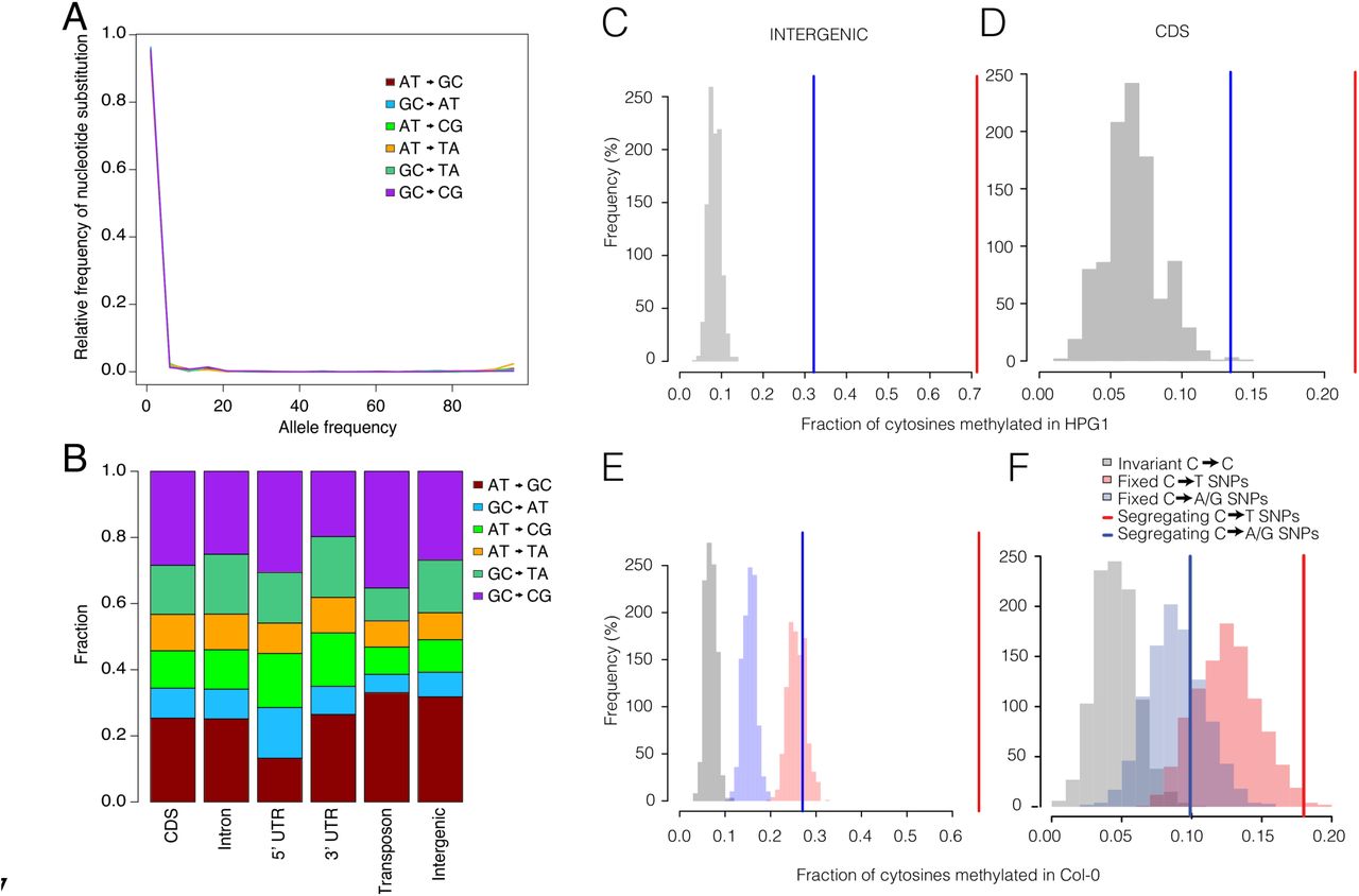
(A) “Unfolded” site frequency spectrum using Arabidopsis lyrata as outgroup for all transitions and transversions. (B) Substitution spectrum for all transitions and transversions divided by genomic annotation. (C, D) Fraction of intergenic SNPs (C) and coding sequence (CDS) SNPs (D) that correspond to methylated cytosines in the HPG-I pseudo-reference. Methylation data was taken from (Hagmann et al., 2015). (E, F) Fraction of intergenic (E) and CDS SNPs (F) that correspond to methylated cytosines in the Col-0 reference genome (methylation data from (Becker et al., 2011)). Blue and red lines indicate fractions for SNPs segregating within the HPGI population. Red and blue histograms indicate fractions for subsets of SNPs fixed within the HPGI population. Grey histograms indicate fractions for invariant positions, i.e., cytosines that have not undergone substitution. See Extended Experimental Procedures for details.
Related to Figure 3.

The line shows the number of SNPs per 100 kb window. Centromere locations are indicated by grey background. Vertical lines indicate SNPs associated with root phenotypes (red) and climatic variables (blue).
Related to Figure 5.

(A, B) The model infers the most probable geographic location of each of the nodes of the phylogeny in Figure 3. (A) Ancestral distribution map summarizing the first ∼100 years of the phylogenetic tree (green). The clouds represent the 95% interval of the Highest Posterior Probability Density of locations. (B) Current distribution map (blue) summarizing the last ∼100 years. Clouds as in (A). (C, D) Diversity in time and space. (C) Diversity in time. Each point represents the average hamming genetic distance among samples within a decade. The black line shows the fit using a generalized additive model and the grey shaded area the 95% confidence interval. (D) Diversity in space. Each point represents the average hamming genetic distance among the 10 geographically closest neighbors. Genetic distances are represented as a scaled gradient from red (low) to blue (high) local genetic diversity.

(A-F) Linkage disequilibrium and SNPs with significant trait associations. Histogram of genetic distances (A) between samples when evaluating only coding regions at 5% minimum allele frequency. Linkage disequilibrium between SNP hits measured as r2 (B) and D’ (C). Three significant SNPs were further studied to exemplify the power of association analyses with HPGI. For each, phenotypic differences between accessions that differ in the focal SNP and that are otherwise virtually genetically identical are compared both with all pairs of accession and with pairs of accessions completely identical for coding regions. Below each violin plot is the histogram of linkage disequilibrium of the focal SNP with all other SNP hits. The three focal SNPs evaluated are inside AT5GI9330 (D), ATIG54440 (E) and AT2GI6580 (F) genes. (G-J) Correlation between SNP effects, frequency and age. Correlation between SNP frequency and p-value (G), frequency and effect (H), age and p-value (I), age and effect (J).
Related to Figure 5.
SUPPLEMENTAL EXPERIMENTAL PROCEDURES
Sample collection
Modern A. thaliana accessions were chosen from the collection described by Platt and colleagues (2010); HPGI candidates were identified based on 149 genome-wide SNPs (Table S1). Seeds were bulked at the University of Chicago. Progeny for DNA extraction was grown at the Max Planck Institute for Developmental Biology. Herbarium specimens (collection dates 1863-1993) were directly sampled by our colleagues jane Devos and Gautam Shirsekar, or sent to us by collection curators (Table S1). We used 2 to 8 mm2 of dried tissue for destructive sampling.
DNA extraction, library preparation and sequencing
DNA from herbarium specimens was extracted in a clean room facility at the University of Tubingen as described (Yoshida et al., 2013). Two sequencing libraries were prepared for each specimen; without and with repair of deaminated sites with uracil-DNA glycosylase and endonuclease VIII (Briggs et al., 2010). DNA from modern, live samples was extracted from rosette leaves pooled from 8 individual plants using the DNeasy plant mini kit (Qiagen, Hilgendorf, Germany). Genomic DNA libraries were prepared using the TruSeq DNA Sample prep kit or TruSeq Nano DNA sample prep kit (illumina, San Diego, CA). Unrepaired herbarium libraries were screened for authenticity by sequencing at low coverage on illumina HiSeq 2500 or MiSeq instruments. Production sequencing (101 bp paired end) was carried out on an illumina HiSeq 2000 instrument.
Read processing
Paired-end reads from modern samples were trimmed and quality filtered before mapping using the SHORE pipeline vO.9.0 (Hagmann et al., 2015; Ossowski et al., 2008). Because ancient DNA fragments are short (Fig. S1B), forward and reverse reads for herbarium samples were merged after trimming, requiring a minimum of 11 bp overlap (Yoshida et al., 2013), and were treated as single-end reads. Reads were mapped with GenomeMapper v0.4.5s (Schneeberger et al., 2009) against an HPGI pseudo-reference genome (Hagmann et al., 2015), and against the Col-0 reference genome. Samples JK2509 to JK2531 were only mapped to the HPGI pseudo-reference genome. Coverage, number of covered positions in the genome, and number of SNPs identified per accession relative to HPGI are reported in Table S1.
We also sequenced the genomes of twelve greenhouse-grown mutation accumulation (MA) lines (Becker et al., 2011; Shaw et al., 2000) (Table S2). We called SNPs, indels and structural variants (SVs), following the workflow and parameters described (Hagmann et al., 2015), but without repeated iterations. This procedure resulted in 2,203 polymorphisms that were shared by all lines, indicating errors in the reference sequence (12% of variants replaced N’s in the TAIR9 genome) or genetic differences in the founder plant of the MA population compared to the Col-0 individual that had been used to generate the reference genome. In addition, we identified 388 segregating variants across the twelve lines (Table S2), of which 350 were singletons. This analysis revealed on average 25.5 SNPs, 4.9 deletions and 3.2 insertions per 31st generation line (Table S2), compared to 19.6 SNPs, 2.4 deletions and 1.0 insertions previously detected in the 30th generation with shorter read length and lower read depth (Ossowski et al., 2010). The genome length accessed in this sequencing effort, 115,954,227,bp, was used to scale the number of point mutations to a rate of 7.1 × 10⁻⁹ mutations site−1 generation−1 (Table S3).
Identification of bona fide HPGI accessions and HPGI phylogeny
We established the relationships among samples at three levels of resolution: (i) the original 149 nuclear SNP genotyping calls based on which the HPGI haplogroup had been identified (Platt et al., 2010), (ii) SNPs in the chloroplast genome (where we did not find any variants), (iii) and all nuclear genome SNPs. At these three levels we performed a multidimensional scaling (MDS) analysis and built a neighbor-joining tree using the adegenet package in R (Jombart et al., 2008).
We used four methods to estimate the relationships among modern accessions, and between modern accessions and historic specimens: (i) multidimensional scaling (MDS) analysis; (ii) construction of a neighbor joining tree with the adegenet package in R (Jombart, 2008), with branch support assessed with 1,000 bootstrap iterations; (iii) construction of a parsimony network using SplitsTree v.4.12.3 (Huson and Bryant, 2006), with confidence values calculated with 1,000 bootstrap iterations; (iv) performing a Bayesian phylogenetic analysis using BEAST v. 1.8 (Bouckaert et al., 2014; Drummond et al., 2012) (see below).
Descriptive genome-wide statistics
We estimated genetic diversity as Watterson’s θ and nucleotide diversity π, and the difference between these two statistics as Tajimas’s D using DnaSP v5 (Librado and Rozas, 2009), both for the entire dataset and independently for modern and herbarium specimens. We calculated the folded and unfolded site frequency spectrum (SFS) for the whole dataset. For the unfolded SFS, we assigned the ancestral state using the Arabidopsis lyrata genome (Hu et al., 2011). We estimated pairwise linkage disequilibrium (LD) between all possible combinations of informative sites, ignoring singletons, by computing r2 D and D’ statistics. LD decay was estimated using a linear regression approach. For the modern individuals, we calculated the recombination parameter R and performed the four-gamete-test (Hudson and Kaplan, 1985) to identify the minimum number of recombination events. All LD and recombination related statistics were determined using DnaSP v5 (Librado and Rozas, 2009).
Substitution and mutation rate analyses
Greenhouse.grown mutation accumulation lines
Mutation rate estimated from greenhouse-grown mutation accumulation lines (Becker et al., 2011) was calculated per line, and the mean and confidence intervals are reported. For each 31st generation MA line, the number of point mutations detected was divided by 31 and by the total genome length. The genome length was determined as all base pairs with coverage higher or equal to 3, and a SHORE mapping quality score of at least 32 in one sample (Table S2).
Natural populations of HPGI
To estimate the number of nucleotide changes per year in natural populations of HPGI, we took advantage of the known collection years of the samples. We used genome-wide nuclear SNPs to calculate pairwise “net” genetic distances between historic and modern HPGI samples using the equation D’ij = Dic-Dij, where D’ij is the net distance between a modern sample i and a historic sample j; Dic the distance between the modern sample i and the reference genome c; and Djc is the distance between a modern sample (j) and the reference genome (c). We calculated a pair-wise time distance in years, Tij, between all modern and historic pairs using the collection dates and linear regression:

The slope coefficient b describes the number of substitution changes per year. However, the points in the regression are not independent because different lines have some common evolutionary history, regression confident intervals would be “over-confident”. We calculated more rigorous 95% confidence intervals using 1000 bootstrap resamples (Drummond et al., 2003). We used either all SNPs or SNPs at specific annotations. To scale the genome-wide substitution rate into a per-base rate, we used all positions that passed SNP or reference call quality thresholds, instead of using a single value of genome length.
The second approach to estimate a substitution rate was framed in Bayesian phylogenetics using the tip-calibration approach implemented in BEAST vl.8 software (Drummond et al., 2012). After systematic runs and chain convergence assessment of different demographic and molecular clock models, we determined that the Skygrid demographic model and the lognormal relaxed molecular clock were the most appropriate. Our analysis simultaneously optimized tree topology and length, substitution rate, and the demographic model. Using the relationship between the time distance of two sequences and the difference in branch length in the tree, BEAST estimates a molecular clock. Under a relaxed molecular clock, the substitution rate is allowed to vary across branches with a lognormal distribution. The prior used for molecular clock was a Continuous-Time Markov Chain (CTMC) (Ferreira and Suchard, 2008). The demographic model is a Bayesian nonparametric demographic model that is optimized for multiple loci, and which allows for complex demographic trajectories by estimating population sizes in time bins (of 10 years in our case) across the tree, based on the number of coalescent events per bin (Gill et al., 2012). In addition, to confirm that demography and root dating converged on the same parameters, we performed a second estimate using a fixed substitution rate of 3.3 × 10⁻⁹ substitutions site−1 years−1 that we had estimated empirically using the net-distance method.
The analysis was carried out remotely at CIPRES PORTAL (v3.l www.phylo.org) using uninformative priors. The run took about 1,344 CPU hours and performed 1,000 million steps in a Monte Carlo Markov Chain (MCMC), sampling every 100,000 steps. Burn-in was adjusted to 10% of steps. To visualize the tree output we produced a Maximum Clade Credibility (MCC) tree with a minimum posterior probability threshold of 0.8 and a 10% burn-in using TreeAnnotator (part of BEAST package), and visualized the MCC tree using FigTree (tree.bio.ed.ac.uk/software/figtree/). Additionally, we used DensiTree (Bouckaert, 2010) to draw simultaneously the 10,000 BEAST trees with the highest posterior probability. Since all trees were drawn transparently, agreements in both topology and branch lengths appear as densely colored regions (Fig. 3A), while areas with little agreement appear lighter.
Demography and migration of HPGI
From the Bayesian phylogenetic analyses described in previous sections, we studied the demographic model estimated via Skygrid. We reconstructed a skyline plot that depicts changes in effective population size, a measure of relative diversity, through time (Bouckaert et al., 2014; Drummond et al., 2012). Implementation of non-phylogenetic methodologies for demographic inference exist, e.g. Multiple sequentially Markovian coalescent (MSMC) (Schiffels and Durbin, 2014), but after exploring them we concluded that their resolution is not sufficient for analyses of the last several centuries, as in our case.
We performed another Bayesian phylogenetic analysis incorporating a geographic location trait (Lemey et al., 2010; Wilson and Barton, 1995). For this, Brownian diffusion parameters are estimated by fitting a continuous gradient of geographic locations along tree branches, starting from the leaves of the tree for which geographic locations are known, i.e. the collection sites of our samples. We excluded three samples from the West coast of the United States, since propagation by Brownian diffusion along large distances is an unrealistic model. We ran this analysis with the parameters described in the previous sections and sliced the resulting 3D (temporal and geographical) phylogeny at the early 16* century and late 18th century using SPREAD software (Bielejec et al., 2011).
We used a heuristic search using an isolation-by-distance pattern inspired by (Handley et al., 2007) to find the origin of diffusion of HPGI in North America, and compared it to the phylogeography analyses. We performed pairwise tests of the relation between genetic and geographic distances using a linear regression. Afterwards we decomposed for each sample the isolation-by-distance pattern (i.e. each row of both distance matrices), and tested whether the slope of the regression still held, that is, whether the remaining samples showed a gradual increase in genetic distance as they moved away from the presumed origin. The sample locations that showed the steepest and most significant slopes were assumed to have been closest to the origin of HPGI diffusion. Because there are indications that more than a single spread of the groups might have happened, we performed the isolation by distance analyses for modern accessions and herbarium specimens separately. These two analyses allowed us to locate the origin of the modern and historic diffusions of HPGI in North America, respectively. The analysis consisted of a heuristic search across all sampled locations, in which a regression between genetic distance ∼ Euclidean geographic distances was performed.
Analysis of the methylation status of mutated sites
As in many other species, the spectrum of de novo mutations in A. thaliana is biased towards G:C→A:T transitions in greenhouse-grown mutation accumulation lines (Ossowski et al., 2010), leading to an inflated transition-to-transversion ratio (Ts/Tv). This bias is less pronounced in recent mutations in a Eurasian collection of natural accessions (Cao et al., 2011) and in HPGI accessions (Fig. 3D). A recent multigenerational salt stress experiment in the greenhouse also showed a more balanced Ts/Tv (Jiang et al., 2014). These findings indicate that less benign conditions might promote a lower Ts/Tv.
The mechanisms underlying a high Ts/Tv ratio are unknown, but could include spontaneous deamination of methylated cytosines (5-methyl-C → T). In agreement with this possibility, we found previously that ancestral cytosines methylated in the A. thaliana reference strain had a more than two-fold higher polymorphism rate than unmethylated cytosines, with the highest rate found in CHG sites (where H is A, C or T) (Table 1, Cao et al., 2011).
We interrogated the putative evolutionary role of cytosine methylation in the mutability of cytosine bases in the HPGI accessions. For reference DNA methylation data, we used previously generated bisulfite-sequencing data of HPGI strains (Hagmann et al., 2015) and of Col-0 lines (Becker et al., 2011), respectively. Our rationale was that if methylation affected mutability, this should reflect in the proportion of mutated sites being methylated in the reference datasets, compared to that proportion for non-mutated sites. To be able to determine the ancestral state of a given site, we only considered positions for which we could determine that state by alignment to the A. lyrata genome (Hu et al., 2011).
The test set of genomic positions consisted of the n sites that were invariant cytosines in A. lyrata and the A. thaliana Col-0 reference genome and whose derived allele was present in at least one HPGI accession (i.e., SNPs segregating within the HPGI population). For these sites, we determined the fraction of methylated cytosines as the number of corresponding sites classified as ‘methylated’ in the HPGI and Col-0 reference datasets, respectively, divided by n.
As a first control set of sites, hence called ‘neutral’, we selected cytosines that were invariant between A. lyrata, Col-0, and all HPGI accessions. A second control set, which we called ‘fixed’, consisted of cytosines that were invariant between A. lyrata and Col-0, and that had mutated and had been fixed in all HPGI accessions. For both control sets we generated empirical distributions of the fraction of sites that were methylated in the HPGI and Col-0 reference datasets, respectively. To this end, we randomly selected n positions with sequence information in the methylation datasets; this process was repeated 1,000 times.
Ancestral cytosines with higher methylation proportion in both A. thaliana and HPGI methylome datasets were more likely to mutate to thymines (Fig. S3C-F). Surprisingly, not only C→T but also C→A/G segregating sites were more likely to have been methylated compared to the fixed and neutral positions, which cannot be explained by higher deamination rates of methylated vs. unmethylated cytosines.
There is an ongoing debate on how epigenetics, i.e. environmentally-induced modification with non-Mendelian inheritance, could contribute to adaptation (Mirouze and Paszkowski, 2011; Nicotra et al., 2010). This result could certainly constitute a genetically-based hypothesis of epigenetic roles in adaptation, perhaps in favor of the “adaptive mutation” argument heavily evidenced in bacteria (Al Mamunetal., 2012).
Inference of genome-wide selection parameters
We estimated the average strength of genome-wide selection using the non-equal relationship between whole-genome and intergenic substitution rates. We selected intergenic regions as the neutral reference because they should not involve any direct phenotypic or biochemical effect but have abundant sites to compare with. This was based on the well-known relationship described by Kimura (1967):
 where k is the substitution rate, μ the mutation rate, Ne the effective population size, and Q the fixation probability of a new mutation. Under neutrality, substitution and mutation rate should be equal since
  and the effective population size term, 2Ne, cancels out in the equation. With a semidominant genome-wide selection coefficient s acting on a new mutation, Q ≈ s / 2Ne (l-e2Nes) (Charlesworth and Charlesworth, 2010). We used the intergenic substitution rate as proxy for the mutation rate μ and the whole-genome substitution rate as proxy for the substitution rate k. We solved the equation for 2Nes, known as the population selection parameter.

Association analyses and dating of newly arisen mutations
For 63 modern accessions, we measured time to bolting and flowering with four replicates, and fecundity (as seed set) with one replicate in growth chambers at the University of Chicago. Additionally, using ≥ 10 replicates we analyzed primary root phenotypes at the Gregor Mendel Institute in Vienna, describing growth and morphological traits extracted from images as described (Slovak et al., 2014) (see next section for details in phenotypic characterization). For associations with climate parameters, we followed a similar rationale as described (Hancock et al., 2011). We extracted information from the publicly available bioclim database (http://www.worldclim.org/bioclim) at 2.5 degrees resolution raster and intersected it with geographic locations of HPGI samples (n = 103).
We performed association analyses using the R package GenABEL (Aulchenko et al., 2007), with measured phenotypes (p = 25) and climatic variables (c = 18) as response variables and SNPs as explanatory variables. A Minimum Allele Frequency cutoff 5% was used. The number of assessed SNPs was 391 in a dataset of only modern samples but imputed genotypes for missing data using Beagle v4.0 (Browning and Browning, 2009), and 456 SNPs with a dataset of modern and also historic samples, although without imputation. For all associations, either phenotypic or climatic ones, minimum 63 individuals were genotyped for a SNP. All phenotypic variables were measured in common chamber or common garden experiments. We first investigated broad sense heritability (H2) of each trait using ANOVA partition of variance between and within lines using replicates (Table S4). Significance was obtained by common F test in ANOVA Secondly we used the polygenic_hglm function in GenABEL to fit a genome wide kinship matrix in order to calculate a narrow sense heritability estimate (h2). Significance was calculated employing a likelihood ratio test comparing with a null model. In principle, h2 is a component of H2, then its values should always be h2 < H2. Our result cannot be interpreted in this framework, since we employed genotype means for h2 calculation and replicate measurements for H2 calculation. This reduced the environmental and developmental noise and thus inflated h2 (Table S4). In this framework, however, we could calculate h2 for climatic variables as well. Seed size had a particularly high heritability, a pattern attributed to highly accurate and replicated measurements (see Phenotyping section). For association analyses we first employed a linear mixed model that fitted the kinship matrix using the mmscore function, and only three significant SNP hits were discovered using a 5% significance threshold after False Discovery Rate correction (FDR). This was expected since we have very few variants and these would have originated in an approximated phylogeny structure. We concluded that fitting the kinship matrix in our model was not appropriate since there would be no leftover variation for association with specific SNPs. With this rationale we employed a fixed effects linear model using the function qtscore from GenABEL. To reduce the false-positive rate we took a conservative permutation strategy that consisted in carrying out association analyses over 1,000 random datasets (permuting phenotypes across individuals) and used the resulting p-value distribution to correct p-values estimated with the original dataset. SNPs with p-values below 5% in the empirical p-value distribution were considered significant (Table S5). In climatic models, we additionally included longitude and latitude as covariates to correct any spurious association between SNPs and climate gradients created by the migratory pattern of isolation by distance. Significant SNPs were interspersed throughout the genome (Fig. S4) and their p-value and phenotypic effect did not correlate with the putative age of the SNPs neither with the frequency, something that could have indicated that the significance was merely driven by the higher statistical power of intermediate frequency variants (Fig. S5 G-J). Using QQ plots to assess inflation or deflation of p-values, we observed generally that permutation corrected p-values were deflated. Straight series of points in QQ plots indicate identical p-values for multiple SNPs, a pattern that we attributed to long range LD, i.e. lack of independence (see Graphical Table S6 for trait distributions and QQ plots from each association analysis). Due to this fact, we add two correction procedures more: (1) Bonferroni-correcting the significance threshold for permutation corrected SNPs from 5% to 5% / number of traits, i.e. 0.2% for phenotype association and 0.27% for climatic associations. (2) Bonferroni-correcting the significance threshold for raw p-values from 5% to 5% / (number of SNPs + number of traits), i.e. 0.01% for phenotype and climatic associations (Table 1 and S5).
For each SNP in our dataset, we determined directionality of mutation, i.e. ancestral vs derived alleles, by determining which state was found in the oldest herbarium samples. We compared the time of emergence and the centroid of geographic distribution of the alternative alleles of SNP hits to random draws of SNPs with the same minimum allele frequency filtering (5%).
On top of phenotypic and climatic associations of SNP hits, we also provide a putative protein effect employing a commonly used amino acid matrix of biochemical effects (Grantham, 1974). Gene name and ontology categorization of SNPs inside annotated transcriptional units was extracted from the online tool www.arabidopsis.org/tools/bulk/go/.
Association analyses – proof of concept examples
We argue that the power of an association approach relies on the fact that HPGI lines resemble Near Isogenic Lines (NILs) produced by experimental crosses (Weigel, 2012). Similarly to genome-wide association studies (GWA), power depends on a number of factors, namely the noise of phenotype under study, architecture of phenotypic trait, quality of genotyping, population structure, sample diversity, sample size, allele frequency, and recombination. On one hand, association analyses in NILs suffers from large linkage blocks, but confident results can be achieved due to accurate measurement of phenotypes, limited genetic differences between any two lines, and high quality genotypes. In common GWA such as in humans, there are multiple confounding effects. Among the confounders are (1) that any two samples differ in hundreds of thousands of SNP and (3) that historical and geographic stratification produce non-random correlations among those SNP differences. This complicates considerably the identification of phenotypic effects at specific genes, and power relies greatly on large samples and frequent recombination between markers.
We exemplify the association analysis confidence with some examples. To provide support for the nonsynonymous SNP on chromosome 5, at position 6,508,329 in AT5GI9330, we looked for pairs of lines that carry the ancestral and the derived allele, but that differ in few (or no other) SNP in the genome. When considering all genic substitutions with a minimum allele frequency of 5% (Fig. S6A), we identified 20 pairs of lines differing only in the AT5G19330 SNP and another linked SNP (which is located on a different chromosome and had an association p-value > 0.4). The phenotypic differences in mean gravitropic score of these almost-identical pairs were significantly higher than phenotypic differences among all pairs of HPGI lines, and genetically identical pairs attending to substitutions inside genes (Fig. S6D). Furthermore this SNP was not in linkage disequilibrium with any other SNP hit (r2 < 0.6) (Fig. S6D). A similar approach was used to examine the SNPs in AT2G02220 (Fig. S6E) and AT2G16580 (Fig. S6F).
Phenotyping
Root phenotypes
Fifteen root phenotypes were scored for three replicates per genotype over a time-series experiment via image analysis as described in detail in (Slovak et al., 2014). We used the mean and standard deviation of the time series values for association analyses.
Seed size phenotype:
We dispersed the seeds of given genotypes on separate plastic square 12 × 12 cm Petri dishes. For faster image acquisition we used cluster of eight Epson V600 scanners. The scanner cluster was operated by the BRAT Multiscan image acquisition tool (https://www.gmi.oeaw.ac.at/research-groups/wolfgang-busch/resources/brat/). The resulting 1600 dpi images were analyzed in Fiji software. Scans were converted to 8-bit binary images, thresholded (parameters: setAutoThreshold(“Default dark”); setThreshold(20, 255)) and particles analyzed (inclusion parameters: size=0.04-0.25 circularity=0.70-1.00). The 2D seed size was measured in square millimeters (parameters: distanced600 known=25.4 pixel=l unit=mm) on > 500 replicates per genotype.
Flowering time in growth chambers
We estimated the flowering time in growth chambers under 4 vernalization treatments. We grew 6 replicates per accession divided between two complete randomized blocks for each treatment. Seeds were sown on a 1:1 mixture of Premier Pro-Mix and MetroMix and cold stratified for 6 days (6°C, no light). We then let plants germinate and grow at 18°C, 14 hours light, 65% humidity. After 3 weeks, we transferred the plants to the vernalization conditions (6°C, 8 hours light, and 65% humidity). The 4 treatments consisted of 0, 14, 28 and 63 days of vernalization, respectively. After the vernalization treatment, plants were transferred back to the previous long day growth conditions. Trays were rotated around the growth chambers every other day throughout the experiments, under both vernalization and growth conditions. Germination, bolting and flowering dates were recorded every other day until all plants had flowered. Days till flowering or bolting times were calculated from the germination date until the first flower bud was developed and until the first flower opened, respectively. The average flowering time and bolting time per genotype was used for association analyses.
Flowering time and fecundity in the field
To investigate variation in flowering time and fecundity in natural conditions, we grew 3 replicates for each of the 78 accessions in a field experiment following a completely randomized block design. Seeds were sowed between 09/20/2012 to 09/22/2012 in 66 well trays (well diameter=4cm) on soil from the field site where plants were to be transplanted. The trays were cold stratified for seven days before being placed in a cold frame at the University of Chicago, IL, USA, (outdoors, no additional light or heat, but watered as needed and protected from precipitation). Seedlings were transplanted directly into tilled ground at the Warren Wood field station (41.84° North, 86.63° West), Michigan, USA on 10/13/2012 and 10/14/2012. Seedlings were watered-in and left to overwinter without further intervention. Plants were scored for bolting and flowering in Spring 2013. Upon maturation of all fruits, stems were harvested and stored between sheets of newsprint paper. To estimate the fecundity, stems were photographed on a black background and the size of each plant was estimated as the number of pixels occupied by the plant on the image. This measure correlates well with the total length of siliques produced, a classical estimator of fecundity in A. thaliana (Spearman’s rho=0.84, p-value<0.001, data not shown).
ACKNOWLEDGEMENTS
For providing and retrieving herbarium specimens, we thank Robert Capers (University of Connecticut), Jane Devos and Gautam Shirsekar (MPI), Michael S. Dossmann (Arnold Arboretum), John Freudenstein (Ohio State University), Cathy M. Herring (Agricultural Research Station, North Carolina State University), Christine Niezgoda (Field Museum), Carol Ann McCormick (University of North Carolina), John Peter (New York Botanical Garden), and Marco Thines (Goethe University). We thank Xiaohui Zhao and Ian Henderson (SLCU) for recombination estimates in Eurasia, Christa Lanz (MPI) for support with sequencing, Christian Goeschl and Bettina Zierfuss (GMI) for assistance in root imaging, and Bonnie Wohlrab (GMI) for amplifying the seeds for root assays. We thank Magnus Nordborg for discussions and pointing us to the work of Templeton, Kay Pruefer for input on data analysis, Patricia Karlsson and Danelle Seymour for thorough proofreading and comments, and various present and past members of the Department of Molecular Biology of the Max Planck Institute for Developmental Biology for further comments on the manuscript. This work was supported by ERC Advanced Grant IMMUNEMESIS and the Max Planck Society.
AUTHOR CONTRIBUTIONS
H.A.B and D.W. conceived and supervised the project, and coordinated the collaborative effort. J.B. coordinated the collection of modern seed samples. C.J. B.B. and J.B. performed and analyzed flowering time and seed set greenhouse experiments. R.S. and W.B. conceived and analyzed root assays. C.S. and R.S. performed the root assays and seed size phenotyping. C.B. and J.H. sequenced and curated modern samples. H.A.B. coordinated the collection and analysis of herbarium samples. J.K. coordinated the extraction of DNA and library preparation of herbarium samples. V.J.S. and E.R. prepared sequencing libraries from herbarium specimens. C.B. called variants in HPGI. J.H. called variants in mutation accumulation lines. M.E.A performed the population and quantitative genomic analyses with supervision of R.N., C.B. and H.A.B. The paper was written by M.E.A, C.B., H.A.B. and D.W. with comments from all coauthors.
REFERENCES
SUPPLEMENTAL REFERENCES


