

ABSTRACT
Eukaryotes carry numerous asexual cytoplasmic genomes (mitochondria and chloroplasts). Lacking recombination, asexual genomes suffer from impaired adaptive evolution. Yet, empirical evidence suggests that cytoplasmic genomes do not suffer this limitation of asexual reproduction. Here we use computational models to show that the unique biology of cytoplasmic genomes—specifically their organization into host cells and their uniparental inheritance–enable them to undergo adaptive evolution more effectively than comparable free-living asexual genomes. Uniparental inheritance decreases competition between different beneficial substitutions (clonal interference), reduces genetic hitchhiking of deleterious substitutions during selective sweeps, and promotes adaptive evolution by increasing the level of beneficial substitutions relative to deleterious substitutions. When cytoplasmic genome inheritance is biparental, a tight transmission bottleneck aids adaptive evolution. Nevertheless, adaptive evolution is always more efficient when inheritance is uniparental. Our findings help explain empirical observations that cytoplasmic genomes—despite their asexual mode of reproduction–can readily undergo adaptive evolution.
1. INTRODUCTION
About 1.5-2 billion years ago, an a-proteobacterium was engulfed by a proto-eukaryote, an event that led to modern mitochondria [1]. Likewise, chloroplasts in plants and algae are derived from a cyanobacterium [2]. These cytoplasmic genomes are essential to extant eukaryotic life, producing much of the energy required by their eukaryotic hosts. Like their ancient ancestors, cytoplasmic genomes reproduce asexually and appear to undergo little recombination with other cytoplasmic genomes [3, 4].
Since they lack recombination, asexual genomes have lower rates of adaptive evolution than sexual genomes unless the size of the population is extremely large [5, 6]. While the theoretical costs of asexual reproduction have long been known [5–9], conclusive empirical evidence is more recent [10–13]. Three factors largely explain why asexual genomes have low rates of adaptive evolution: (1) beneficial substitutions accumulate slowly; (2) deleterious substitutions are poorly selected against; and (3) when beneficial substitutions do spread, any linked deleterious substitutions also increase in frequency through genetic hitchhiking [5, 7, 8, 10, 11].
The lack of recombination in asexual genomes slows the accumulation of beneficial substitutions. Recombination can aid the spread of beneficial substitutions by separating out rare beneficial mutations from deleterious genetic backgrounds (“ruby in the rubbish”) [14]. Furthermore, recombination can reduce competition between different beneficial substitutions (“clonal interference”) [5, 7, 8, 10, 11, 15–17]. Under realistic population sizes and mutation rates, an asexual population will contain multiple genomes—each with different beneficial substitutions—competing with one another for fixation [11, 16]. Ultimately, clonal interference leads to the loss of some beneficial substitutions, reducing the efficiency of adaptive evolution [5, 7, 8, 10, 11, 15–17].
The lack of recombination also makes it more difficult for asexual genomes to purge deleterious substitutions. An asexual genome can only restore a loss of function from a deleterious substitution through a back mutation or a compensatory mutation, both of which are rare [5, 18]. Unless the size of the population is very large, the number of slightly deleterious substitutions should increase over time as the least-mutated class of genome is lost through genetic drift (“Muller’s ratchet”) [5, 18].
If that were not enough, asexual genomes are also especially susceptible to genetic hitchhiking [10, 11], a process by which deleterious substitutions spread through their association with beneficial substitutions [19, 20]. As all loci on an asexual genome are linked, deleterious and beneficial substitutions on the same genome will segregate together. When the positive effect of a beneficial substitution outweighs the negative effect of a deleterious substitution, the genome that carries both can spread through positive selection [19, 20]. Even when the additive effect is zero or negative, a beneficial substitution can still aid the spread of a deleterious substitution via genetic drift by reducing the efficiency of selection against the deleterious substitution. Genetic hitchhiking can thus offset the benefits of accumulating beneficial substitutions by interfering with the genome’s ability to purge deleterious substitutions [19, 20].
Free-living asexual organisms (e.g. bacteria) generally have very large population sizes [21], allowing these organisms to alleviate some of the costs of asexual reproduction [5, 6]. Asexual cytoplasmic genomes, however, have an effective population size much smaller than that of free-living asexual organisms [21, 22]. As a smaller population size increases the effect of genetic drift, cytoplasmic genomes should have less efficient selection than asexual organisms [23, 24] and should struggle to accumulate beneficial substitutions and to purge deleterious substitutions [25–27].
But despite theoretical predictions, cytoplasmic genomes readily undergo adaptive evolution. Mitochondrial protein-coding genes show signatures that are consistent with both low levels of deleterious substitutions [21, 28, 29] and frequent selective sweeps of beneficial substitutions [30, 31]. Indeed, it is estimated that 26% of mitochondrial substitutions that alter proteins in animals have become fixed through adaptive evolution [32]. Beneficial substitutions in the mitochondrial genome have helped animals adapt to specialized metabolic requirements [33–36] and have enabled humans to adapt to cold northern climates [37]. Likewise, it is clear that adaptive evolution has played a role in the evolution of chloroplast genomes [38, 39].
How then do we reconcile empirical evidence for adaptive evolution in cytoplasmic genomes with theoretical predictions that such adaptation should be impaired? Unlike free-living asexual organisms, which are directly exposed to selection, cytoplasmic genomes exist within host cells. The fitness of cytoplasmic genomes is therefore closely aligned with the fitness of their host. Each of these hosts carries multiple cytoplasmic genomes that are generally inherited from a single parent (uniparental inheritance) [40]. During gametogenesis, cytoplasmic genomes can undergo tight population bottlenecks, affecting the transmission of genomes from parent to offspring [41, 42]. Cytoplasmic genomes are thus subject to very different evolutionary pressures than free-living asexual organisms.
Some of the effects of uniparental inheritance and a transmission bottleneck on the evolution of cytoplasmic genomes have already been identified. Both uniparental inheritance and a transmission bottleneck decrease within-cell variance in cytoplasmic genomes and increase between-cell variance. [40, 43–45]. Uniparental inheritance is known to select against deleterious mutations [44–47] and select for mito-nuclear coadaptation [48]. Similarly, a transmission bottleneck and other forms of within-generation drift are known to slow the accumulation of deleterious substitutions in cytoplasmic genomes [26, 43, 49].
Although the effect of uniparental inheritance and a bottleneck on the accumulation of deleterious substitutions is reasonably well-studied, much less attention has been paid to the other limitations of asexual reproduction: slow accumulation of beneficial substitutions and high levels of genetic hitchhiking. The two studies that have addressed the spread of beneficial substitutions have come to contradictory conclusions. Takahata and Slatkin [49] showed that within-generation drift promoted the accumulation of beneficial substitutions. In contrast, Roze and colleagues [44] found that within-generation drift due to a bottleneck reduced the fixation probability of a beneficial mutation. Takahata and Slatkin found no difference between uniparental and biparental inheritance of cytoplasmic genomes [49] while Roze and colleagues found that uniparental inheritance increased the fixation probability of a beneficial mutation and its frequency at mutation-selection equilibrium [44]. Of the two previous studies, only the model of Takahata and Slatkin was able to examine the accumulation of substitutions [49] (the model of Roze and colleagues only considered a single locus [44]). To our knowledge, no study has looked at how inheritance mode affects genetic hitchhiking in cytoplasmic genomes.
Here we develop theory that explains how cytoplasmic genomes are capable of adaptive evolution despite their lack of recombination. We will show how the biology of cytoplasmic genomes—specifically their organization into host cells and their uniparental inheritance—allows them to accumulate beneficial substitutions and to purge deleterious substitutions more efficiently than comparable free-living asexual genomes.
2. MODEL
For simplicity, we base our model on a population of diploid single-celled eukaryotes. We examine the accumulation of beneficial and deleterious substitutions in an individual-based computational model that compares uniparental inheritance of cytoplasmic genomes with bi-parental inheritance (the presumed ancestral state [40]). Since genetic drift plays an important role in the spread of substitutions, we take stochastic effects into account. We vary the size of the transmission bottleneck during meiosis (i.e. the number of cytoplasmic genomes passed from parent to gamete) to alter the level of genetic drift. To examine how the organization of cytoplasmic genomes into host cells affects their evolution, we also include a model of comparable free-living asexual genomes.
We have four specific aims. We will determine how inheritance mode and the size of the transmission bottleneck affect (Aim 1) clonal interference and the accumulation of beneficial substitutions; (Aim 2) the accumulation of deleterious substitutions; (Aim 3) the level of genetic hitchhiking; and (Aim 4) the level of adaptive evolution, which we define as the ratio of beneficial to deleterious substitutions. Although uniparental inheritance and a transmission bottleneck are known to select against deleterious mutations on their own [26, 43–47, 49], the interaction between inheritance mode, transmission bottleneck, and the accumulation of deleterious substitutions has not to our knowledge been examined. Thus we include Aim 2 to specifically examine interactions between inheritance mode and size of the transmission bottleneck. To address our aims, we built four variations of our model. First, we examine clonal interference and the accumulation of beneficial substitutions using a model that considers beneficial but not deleterious mutations (Aim 1). Second, we consider deleterious but not beneficial mutations to determine how inheritance mode and a transmission bottleneck affect the accumulation of deleterious substitutions in cytoplasmic genomes (Aim 2). Third, we combine both beneficial and deleterious substitutions. This allows us to examine the accumulation of deleterious substitutions in the presence of beneficial mutations (genetic hitchhiking; Aim 3) and the ratio of beneficial to deleterious substitutions (Aim 4). For all aims, we compare our models of cytoplasmic genomes to a comparable population of free-living asexual genomes. This serves as a null model, allowing us to examine the strength of selection when asexual genomes are directly exposed to selection.
The population contains N individuals, each carrying the nuclear genotype Aa, where A and a are selfincompatible mating type alleles. Diploid cells contain n cytoplasmic genomes, and each genome has l linked base pairs. A cytoplasmic genome is identified by the number of beneficial and deleterious substitutions it carries (α and κ respectively; note, we do not track where on the genome the mutations occur). Cells are identified by the number of each type of cytoplasmic genome they carry. The life cycle has four stages, and a complete passage through the four stages comprises a generation. The first stage is mutation. Initially, all cells carry cytoplasmic genomes with zero substitutions. Mutations can occur at any of the l base pairs. The probability that one of these l sites will mutate to a beneficial or deleterious site is given by μb and μd per site per generation respectively (determined via generation of random numbers within each simulation). As the mutation rate in mitochondrial DNA is between 7.8 × 10⁻⁸ and 1.7 × 10⁻⁷ per nucleotide per generation [50 –52], we let = 1 × 10⁻⁷ per nucleotide per generation. We assume the beneficial mutation rate is lower than the deleterious mutation rate, and as such, examine both = 1 × 10⁻⁸ and = 1 × 10⁻⁹ per nucleotide per generation [53].

Additional parameters: n = 50, sb = sd = 0.1, γ = 5. A. The three fitness functions used in this study in the case of beneficial mutations only. The selection coefficient is defined such that 1 — sb represents the fitness of a cell with zero beneficial substitutions (a cell with nγ beneficial substitutions has a fitness of 1, where n is the number of cytoplasmic genomes and γ is the number of substitutions each cytoplasmic genome must accumulate before the simulation is terminated). In this case, where n = 50 and γ = 5, a cells fitness is 1 when each cytoplasmic genome in the cell carries an average of 5 substitutions (50 × 5 = 250 beneficial substitutions in total). B. The deleterious fitness function. Here, a cell with no deleterious substitutions has a fitness of 1, while a cell with nγ substitutions has a fitness of 1 — sd. We only examine a concave down decreasing function for the accumulation of deleterious substitutions (unless we are comparing cytoplasmic genomes to free-living genomes, in which case we use a linear fitness function). C. One of the fitness functions used in the model with both beneficial and deleterious mutations. The beneficial substitution portion of the function can take any of the forms in panel A while the deleterious substitution portion takes the form in panel B. In this example the fitness surface combines a linear function for beneficial substitutions with a concave down fitness function for deleterious substitutions. The color represents the fitness of a cell carrying a given number of deleterious substitutions (x-axis) and beneficial substitutions (y-axis). Equations for the fitness functions can be found in SI Text 1.2 (A), SI Text 2 (B), and SI Text 3.2 (C)
After mutation, cells are subject to selection, assumed for simplicity to act only on diploid cells. We assume that each substitution has the same effect, which is given by the selection coefficient (sb for beneficial and sd for deleterious) and that fitness is additive. We assume that a cell’s fitness depends on the total number of substitutions carried by its cytoplasmic genomes. As there are few data on the distribution of fitness effects of beneficial substitutions in cytoplasmic genomes, we examine three fitness functions: concave up, linear, and concave down (Fig. 1A). For deleterious substitutions in cytoplasmic genomes, there is strong evidence that fitness is only strongly affected when the cell carries a high proportion of deleterious genomes [54], and so we use a decreasing concave down function to model deleterious substitutions (Fig. 1B). When we combine beneficial and deleterious mutations in a single model, we examine all three fitness functions for the accumulation of beneficial substitutions but only a concave down decreasing fitness function for the accumulation of deleterious substitutions (Fig. 1B).
We focus on selection coefficients that represent mutations with small effects on fitness: sb = 0.01-0.1 (see the legend of Fig. 1 for a description of how the selection coefficient relates to fitness). Cells are assigned a relative fitness based on the number of beneficial and deleterious substitutions carried by their cytoplasmic genomes. These fitness values are used to sample N new individuals for the next generation.
Each of the post-selection diploid cells then undergoes meiosis to produce two gametes, one with nuclear allele A and the other with nuclear allele a. Each gamete also carries b cytoplasmic genomes sampled with replacement from the n cytoplasmic genomes carried by the parent cell (with b ≥ n/2) [41]. We examine both a tight transmission bottleneck (b = n/10) and a relaxed transmission bottleneck (b = n/2). To maintain population size at N, each diploid cell produces two gametes.
During mating, each gamete produced during meio-sis is randomly paired with another gamete of a compatible mating type. These paired cells fuse to produce diploid cells. Under biparental inheritance, both the gametes with the A and a alleles pass on their b cytoplasmic genomes, while under uniparental inheritance, only the b genomes from the gamete with the A allele are transmitted. Finally, n genomes are restored to each new diploid cell by sampling n genomes with replacement from the genomes carried by the diploid cell after mating (2b under biparental inheritance and b under uniparental inheritance). The model then repeats, following the cycle of mutation, selection, meiosis, and mating described above.
To ensure that our model of free-living asexual genomes can be directly compared to our model of cytoplasmic genomes, we assume a population size of N × n free-living genomes. Each free-living genome carries one haploid asexual nuclear genome with l base pairs. Now there are only two stages to the life cycle: mutation and selection. Mutation proceeds as in the model of cytoplasmic genomes. Selection, however, now depends only on the number of substitutions carried by a genome. We assume that a mutation has the same effect on the fitness of a free-living cell as a mutation on a cytoplasmic genome has on the fitness of its host cell. (When comparing free-living and cytoplasmic genomes, we always use a linear fitness function for both beneficial and deleterious substitutions because for this function the strength of selection on a new substitution is independent of existing substitution load.) Our intention is not to accurately model extant populations of free-living asexual organ-isms, as these differ in a number of ways from cytoplasmic genomes (e.g. population size, mutation rate, and genome size [21]), but rather to examine how the organization of multiple cytoplasmic genomes within a host affects their evolution.

Parameters: N = 1000, n = 50, = 10−8, linear fitness function, and b =25 (relaxed transmission bottleneck) or b = 5 (tight transmission bottleneck). As neither fitness function nor selection coefficient qualitatively affect the results, we show a single representative set of parameter values. Error bars represent standard error of the mean. A. Variance in the number of different cytoplasmic genomes carried by cells (averaged over all cells in the population each generation). As free-living cells carry a single genome, they have no within-cell variance. B. Variance of all cells’ fitness values (averaged over each generation). C. The number of generations separating the genome carrying α substitutions from the genome carrying α + 1 (averaged over all observed substitutions, but excluding α = 1, as the dynamics of α = 1 are largely driven by the starting conditions). The establishment phase begins when the genome carrying α substitutions first appears and ends when that genome becomes established in the population (depicted in dark blue). The sweep phase begins with the establishment of the genome with α substitutions and ends upon the first appearance of the genome with α +1 substitutions (depicted in yellow). D. During the establishment period of the genome with α substitutions, D shows the probability of losing all genomes with α substitutions (P(lose α)) and the probability of regenerating at least one genome with a substitutions once all genomes with α substitutions have been lost (P(regain α)) (averaged over all observed establishment periods, but excluding α =1). E. During the establishment period of the genome with α substitutions, E shows the trajectory of the genome with α − 1 substitutions. To calculate the curves, we divided each of the 500 Monte Carlo simulations into 20 equidistant pieces. We rounded to the nearest generation and obtained the frequency of the genome with α − 1 substitutions at each of those 20 generation markers. Each curve shows the average of those 20 generation markers (over all establishment periods, excluding α =1, and over all simulations) and is plotted so that the end of the curve aligns with the mean length of the establishment period (shown in panel C). F. The mean number of generations to accumulate a single beneficial substitution. We divide the number of generations to accumulate 7 substitutions by the mean number of beneficial substitutions accumulated in that time period (averaged over all simulations).
When we consider beneficial mutations only (Aim 1), the simulation stops once every cytoplasmic genome in the population has accumulated at least 7 beneficial substitutions. For the remaining models, we run each simulation for 10,000 generations. For all the models, we average the results of 500 Monte Carlo simulations for each combination of parameter values (we vary N, n, b, sb, sd, and the fitness functions associated with beneficial substitutions). We wrote our model in R version 3.1.2 [55]. For a detailed description of the model, see SI Text.
3. RESULTS
3.1. Cytoplasmic genomes accumulate beneficial mutations faster than free-living genomes
The units of selection differ between cytoplasmic genomes (eukaryotic host cell) and free-living genomes (free-living asexual cell). Cytoplasmic genomes have two levels at which variance in fitness can be generated: variation in the number of substitutions per genome and variation in the relative number of each genome type in a host cell (Fig. 2A). In contrast, free-living genomes can differ only in the number of substitutions carried per genome. Consequently, cytoplasmic genomes have a greater potential for creating variance between the units of selection than free-living genomes (Fig. 2B).
For conceptual purposes, we break down the accumulation of beneficial substitutions into two phases. In the first phase (establishment), we determine the time for a genome that carries α substitutions to become established in a population that contains genomes with α — 1 or fewer beneficial substitutions. Since we examine small selection coefficients, drift dominates the fate of genomes when they are rare, and the genome with α substitutions is frequently lost to drift when it first arises. The establishment phase starts when we first observe a genome with α substitutions and ends when that genome persists in the population (i.e. it is no longer lost to drift). The second phase (sweep) starts at this point and ends when a genome carrying α + 1 substitutions first appears in the population. Once a genome with α +1 substitutions appears, the establishment phase of this genome begins and the cycle continues.
In cytoplasmic genomes, fewer generations separate the appearance of the genome with α and the genome with α +1 substitutions than in free-living genomes (Fig. 2C). Cytoplasmic genomes more easily become established in the population not because they are less likely to be lost by drift—in fact cytoplasmic genomes are more frequently lost to drift than free-living genomes—but because once a genome with α substitutions has been lost, it is more quickly regenerated (Fig. 2D). The regeneration of the genome with α substitutions is proportional to the rate at which mutations occur on the genome with α − 1 substitutions. In cytoplasmic genomes, the genome with α −1 substitutions increases in frequency much more quickly than in free-living genomes (Fig. 2E). Thus, in cytoplasmic genomes, the genome with α − 1 substitutions presents a larger target for de novo mutations, driving regeneration of the genome with α substitutions (Fig. 2D). As a result, cytoplasmic genomes suffer less from clonal interference (Fig. 3) and take less time to accumulate beneficial substitutions than free-living genomes (Fig. 2F)

Parameters: N = 1000, n = 50, sb = 0:1, and a linear fitness function. The figure depicts a time-series of a single simulation, showing the proportions of genomes carrying different numbers of substitutions (we chose the first completed simulation for each comparison). To quantify the slope of declines in proportion of a genome type (equivalently, the speed at which a genome type is replaced), we report the generations (± se) for the wild type genome to drop from 100% to below 0.5% (averaged over all simulations), which we call g0:005. We also report the mean number of genomes (± se) co-existing in the population (averaged over each generation and over all simulations), which we call cg. A. In a free-living population, genomes with beneficial substitutions spread slowly through the population (g0:005 = 5708 ± 31 generations). As a result, multiple genomes co-exist at any one time (cg = 7:0±0:02 genomes), increasing the scope for clonal interference. B−C. Biparental inheritance with a relaxed bottleneck (B; b = 25) and tight bottleneck (C; b = 5). Genomes with beneficial substitutions spread more quickly compared to free-living genomes (B: g0:005 = 2584 ± 21 generations; C: g0:005 = 1377 ± 14 generations), reducing the number of co-existing genomes (B: cg = 4:8 ± 0:02 genomes; C: cg = 3:8 ± 0:01 genomes). D—E. Uniparental inheritance with a relaxed bottleneck (D; b = 25) and tight bottleneck (E; b = 5). Under uniparental inheritance, genomes with beneficial substitutions spread much more quickly than free-living and biparentally inherited cytoplasmic genomes (D: g0:005 = 463±6 generations; E: g0:005 = 453± generations). This leads to fewer genomes co-existing in the population (D: cg = 3:1 ± 0:01 genomes; E: cg = 2:8 ± 0:01 genomes) and low levels of clonal interference.
3.2. Uniparental inheritance of cytoplasmic genomes promotes the accumulation of beneficial substitutions
Meiosis introduces variation in the cytoplasmic genomes that are passed to gametes. Gametes can thus carry a higher or lower proportion of beneficial substitutions than their parent. Uniparental inheritance maintains this variation in offspring, reducing within-cell variation (Fig. 2A) while increasing between-cell variation (Fig. 2B). Biparental inheritance, however, combines the cytoplasmic genomes of different gametes, destroying much of the variation produced during meiosis and reducing between-cell variation (Fig. 2B). Thus, selection is more efficient when inheritance is uniparental because there is more between-cell variation in fitness on which selection can act (Fig. 2B). Uniparental inheritance eases the establishment of the genome with α substitutions (Fig. 2C) by increasing the rate at which the genome with α substitutions is regenerated once lost to genetic drift (Fig. 2D). Under uniparental inheritance, the genome with α − 1 substitutions quickly increases in frequency (Fig. 2E), driving the formation of the genome with α substitutions. Uniparental inheritance decreases clonal interference (Fig. 3), reducing the time to accumulate beneficial substitutions compared to biparental inheritance (Fig. 2F; see Fig. S1 for a range of different parameter values).
3.3. Inheritance mode is more important than the size of the bottleneck
Under biparental inheritance, a tight bottleneck decreases the variation in cytoplasmic genomes within gametes (Fig. 2A) and increases the variation between gametes (Fig. 2B). Consequently, under biparental inheritance beneficial substitutions accumulate more quickly than when the transmission bottleneck is relaxed (Fig. 2F and Fig. S1). Bottleneck size has less of an effect on uniparental inheritance because uniparental inheritance efficiently maintains the variation generated during meio-sis even when the bottleneck is relaxed (Fig. 2B). When n is larger (n = 200), a tight bottleneck reduces the time for beneficial substitutions to accumulate, but even here the effect is minor (Fig. S1C).
Importantly, the accumulation of beneficial substitutions under biparental inheritance and a tight bottleneck is always less effective than under uniparental inheritance, irrespective of the size of the bottleneck during uniparental inheritance (Fig. 2 and Fig. S1). While a tight transmission bottleneck reduces within-gamete variation, the subsequent mixing of cytoplasmic genomes due to biparental inheritance means that cells have higher levels of within-cell variation and lower levels of between-cell variation than uniparental inheritance (Fig. 2A-B).
3.4. Varying parameter values does not alter patterns
The choice of fitness function has little effect on our findings (Fig. S1). Likewise, varying the selection coefficient does not affect the patterns, although the relative advantage of uniparental inheritance over biparental inheritance is larger for higher selection coefficients (Fig. S1). Increasing the number of cytoplasmic genomes (n) increases the relative advantage of uniparental inheritance over biparental inheritance, whereas increasing the population size (N) has little effect (compare Fig. S1C with Fig. S1A).

Parameters (unless otherwise stated): N = 1000, n = 50, μ = 10−7, a concave down fitness function, and b =25 (relaxed transmission bottleneck) or b =5 (tight transmission bottleneck). A. Comparison with free-living genomes (linear fitness function for both free-living and cytoplasmic genomes and sd = 0.1). B. Mean deleterious substitutions per cytoplasmic genome for sd = 0.1. C. Mean deleterious substitutions per cytoplasmic genome for sd = 0.01. Error bars are ± standard error of the mean.
3.5. Uniparental inheritance helps cytoplasmic genomes purge deleterious substitutions
Free-living asexual genomes accumulate deleterious substitutions more quickly than cytoplasmic genomes (Fig. 4A). Biparental inheritance of cytoplasmic genomes causes deleterious substitutions to accumulate more quickly than when inheritance is uniparental (Fig. 4). A tight transmission bottleneck slows the accumulation of deleterious substitutions under biparental inheritance, but biparental inheritance always remains less efficient than uniparental inheritance at purging deleterious substitutions (Fig. 4).

ϕ < 1 indicates the presence of genetic hitchhiking (the lower the value of ±, the greater the level of hitchhiking). Parameters: N = 1000, n = 50, μb = 10−8, μd = 10−7, and b =25 (relaxed transmission bottleneck) or b = 5 (tight transmission bottleneck). The overall level of genetic hitchhiking in each population, measured by our genetic hitchhiking index (see Fig. S2 for details). Error bars are ± standard error of the mean. A. Free-living comparison (linear fitness function for both beneficial and deleterious substitutions with sb = sb = 0.1). For cytoplasmic genomes, B shows sb = 0.1 while C shows sb = 0.01. For B−C, the fitness function for beneficial substitutions is shown on the x-axis while the fitness function for deleterious substitutions is concave down.
3.6. Uniparental inheritance reduces hitchhiking of deleterious substitutions during selective sweeps
To detect levels of genetic hitchhiking in cytoplasmic genomes, we identified the location of all “beneficial sweeps”, defined as the generation at which the genome that carries the fewest beneficial substitutions is lost from the population. Likewise, we identified the location of all “deleterious sweeps”, which is the generation in which the genome carrying the fewest deleterious substitutions is lost (note that a deleterious sweep is the same as a “click” of Muller’s ratchet [18]) (Fig. S2).
Cycling through each beneficial sweep, we identified the location of the nearest upstream deleterious sweep (i.e. in the same or in a later generation as the beneficial sweep). We measured the number of generations separating the two events and calculated the mean generations of all such instances. To obtain a “genetic hitchhiking index” (ϕ), we normalized by dividing the mean generations by the expected number of generations for a deleterious sweep to follow a beneficial sweep (see Fig. S2 legend for how we calculate the expected number of generations). If fewer than expected generations separated the beneficial and deleterious sweeps (ϕ < 1), we infer that deleterious substitutions benefited from the spread of beneficial substitutions (i.e. genetic hitchhiking occurred) (Fig. S2A). If the expected number of generations separated the beneficial and deleterious sweeps (ϕ ≈ 1), we infer that the spread of beneficial substitutions had little or no effect on the spread of deleterious substitutions (Fig. S2B; see Table S1 for a benchmark of the index using randomly simulated beneficial and deleterious sweeps). If greater than expected generations separated the beneficial and deleterious sweeps (ϕ > 1), we infer that deleterious substitutions were inhibited by the spread of beneficial substitutions (Fig. S2C). For details of our genetic hitchhiking index, see Fig. S2.

Parameters: N = 1000, n = 50, μb = 10 ‘8, μb = 10−7, b = 25, a concave down fitness function for the accumulation of beneficial substitutions, and sb = 0.1 (A) or sb = 0.01 (B). A histogram that shows the distribution of hitchhiking index values for each pair of beneficial and deleterious sweeps. A beneficial sweep occurs when the genome with the fewest beneficial substitutions is lost and a deleterious sweep occurs when the genome with the fewest deleterious substitutions is lost. In both A and B, uniparental inheritance more often leads to cases in which a beneficial sweep is very closely followed by a deleterious sweep (leftmost bar). However, uniparental inheritance also leads to more cases in which the deleterious sweep is greatly separated from the beneficial sweep, indicating that genetic hitchhiking is more often suppressed under uniparental inheritance (right-hand side of the graph). Overall, uniparental inheritance leads to a higher overall hitchhiking index (ϕ)-and thus lower levels of hitchhiking—than biparental inheritance (A. UPI: 0.79; BPI: 0.59. B. UPI: 0.86; BPI: 0.61). Blue bars pertain to uniparental inheritance, the light pink bars pertain to biparental inheritance, and the dark red bars depict overlapping bars (the dark red bar pertains to whichever color does not show on the top of the bar). (We do not plot cases in which the simulation terminates before a beneficial sweep is followed by a deleterious sweep. However, we do take these into account when generating the hitchhiking index value: see Fig. S2 for details.)
In all cases, ϕ < 1 (Fig. 5 and S3), indicating that genetic hitchhiking plays an important role in aiding the spread of deleterious substitutions. Free-living genomes experience higher levels of hitchhiking than cytoplasmic genomes (Fig. 5A). Uniparental inheritance reduces levels of genetic hitchhiking compared to biparental inheritance (Figs. 5B-C, S3). Uniparental inheritance actually increases the proportion of deleterious substitutions that sweep concurrently with beneficial substitutions (Fig. 6; leftmost bar). This occurs when the genomes that sweep carry more than the minimum deleterious substitutions in the population. However, uniparental inheritance also increases the proportion of deleterious sweeps in which ϕ is large (Fig. 6), which occur when the genomes that sweep carry the minimum number of deleterious substitutions in the population. Overall, the latter outweigh the former, leading to lower levels of genetic hitchhiking under uniparental inheritance (Figs. 5, S3).
3.7. Uniparental inheritance promotes adaptive evolution
Cytoplasmic genomes have higher levels of adaptive evolution than free-living genomes under the same set of conditions (Fig. 7A). Strikingly, uniparental inheritance of cytoplasmic genomes leads to a ratio of beneficial to deleterious substitutions that is two orders of magnitude higher than in free-living genomes (Fig. 7A). Among cytoplasmic genomes, uniparental inheritance always leads to higher levels of adaptive evolution than biparental inheritance (Figs. 7, S4). While a tight transmission bottleneck combined with biparental inheritance increases the ratio of beneficial to deleterious substitutions, bi-parental inheritance always has lower levels of adaptive evolution than uniparental inheritance, regardless of the size of the transmission bottleneck (Fig. S4).
4. DISCUSSION
Both theory and experiments indicate that asexual reproduction leads to lower rates of adaptive evolution than sexual reproduction [5, 7, 8, 10, 11, 15–17]. Free-living asexual organisms typically have huge population sizes, allowing them to overcome these limitations of asexual reproduction [21]. Cytoplasmic genomes, however, have much smaller effective population sizes and should be especially susceptible to these limitations of asexual reproduction [25–27]. These predictions, however, are inconsistent with empirical observations that cytoplasmic genomes can readily accumulate beneficial substitutions and purge deleterious substitutions [28, 30, 32, 34].
In this study, we help reconcile theory with empirical observations. We show that the specific biology of cytoplasmic genomes-in particular uniparental inheritance and their organization within hosts-increases the efficacy of selection on cytoplasmic genomes relative to comparable free-living genomes. Furthermore, we show that the mode of inheritance of cytoplasmic genomes has a profound effect on adaptive evolution: uniparental inheritance reduces variation of cytoplasmic genomes within cells and increases variation of fitness between cells, improving the efficacy of selection relative to biparental inheritance.
In particular, uniparental inheritance reduces competition between different beneficial substitutions (clonal interference), causing beneficial substitutions to accumulate on cytoplasmic genomes more quickly than under bi-parental inheritance. Uniparental inheritance also facilitates selection against deleterious substitutions, slowing the progression of Muller’s ratchet. Finally, uniparental inheritance reduces the level of genetic hitchhiking in cytoplasmic genomes, a phenomenon to which asexual genomes are especially susceptible [10, 11]. Lower levels of hitchhiking under uniparental inheritance means that beneficial (selective) sweeps are less likely to involve excess deleterious substitutions. As these genomes lacking excess deleterious substitutions spread, they remove standing variation in the population, purging genomes that carry excess deleterious substitutions and slowing Muller’s ratchet. Furthermore, both theoretical [56] and empirical [57] evidence suggest that beneficial substitutions can slow Muller’s ratchet by compensating for deleterious substitutions. By increasing the ratio of beneficial to deleterious substitutions, uniparental inheritance effectively increases the ratio of beneficial compensatory substitutions to deleterious substitutions. Thus, the accumulation of beneficial substitutions in cytoplasmic genomes not only aids adaptive evolution [32] but improves the ability of cytoplasmic genomes to resist Muller’s ratchet [43, 56]. Our findings thus help explain how cytoplasmic genomes are able to undergo adaptive evolution in the absence of sex and recombination.

Parameters: N = 1000, n = 50, μb = 10−8, μd = 10−7, sb = 0.1, and b = 25 (relaxed transmission bottleneck) or b = 5 (tight transmission bottleneck). A. Comparison with free-living genomes. Here, the fitness function for both beneficial and deleterious substitutions is linear. B—E shows the mean trajectory of the 500 simulations plotted every 500 generations. Here, the fitness function for beneficial substitutions is linear while the fitness function for deleterious substitutions is concave down, decreasing. We calculate the ratio of beneficial to deleterious substitutions as follows. First, we calculate the aggregated mean of the number of beneficial and deleterious substitutions for the population at generation 10,000 (average substitutions per cytoplasmic genome). Second, for each of the 500 simulations we divide the mean number of beneficial substitutions per genome by the corresponding mean number of deleterious substitutions per genome. Finally, we take the average of the ratios of the 500 simulations.
We explicitly included a transmission bottleneck as previous theoretical work seemed to suggest that this alone could act to slow the accumulation of deleterious substitutions on cytoplasmic genomes [43]. Separate work found that host cell divisions-which act similarly to a transmission bottleneck-promoted the fixation of beneficial mutations and slowed the accumulation of deleterious mutations [49]. In contrast, yet another study found that a tight bottleneck increases genetic drift, reducing the fixation probability of a beneficial mutation and increasing the fixation probability of a deleterious mutation [44]. Here we show that these apparently contradictory findings are entirely consistent. We find that a tight transmission bottleneck indeed increases the rate at which beneficial substitutions are lost when rare (Fig. 2D). But in a population with recurrent mutation, losing beneficial mutations when rare can be compensated for by a higher rate of regeneration, explaining how a tight bottleneck promotes adaptive evolution despite higher levels of genetic drift. Although a tight transmission bottleneck promoted beneficial substitutions and opposed deleterious substitutions when inheritance was biparental, we show that a bottleneck must be combined with uniparental inheritance to maximize adaptive evolution in cytoplasmic genomes. A transmission bottleneck is less effective in combination with biparental inheritance because the mixing of cytoplasmic genomes after syngamy largely destroys the variation generated between gametes during meiosis. For the parameter values we examined, uniparental inheritance is the key factor driving adaptive evolution, as the size of the bottleneck has little effect on the accumulation of beneficial and deleterious substitutions when inheritance is uniparental.
Our work illustrates that population genetic theory from free-living organisms cannot be blindly applied to cytoplasmic genomes. Consider effective population size (Ne). A lower Ne leads to higher levels of genetic drift [23], and it is often assumed that low Ne impairs selection in cytoplasmic genomes [24]. However, this assumes that factors which decrease Ne do not alter selective pressures and aid adaptive evolution in other ways. This assumption is violated in cytoplasmic genomes as halving the Ne of cytoplasmic genomes-the difference between biparental and uniparental inheritance-improves the efficacy of selection and can increase the ratio of beneficial to deleterious substitutions by 2-21 times (Fig. S4).
Although our findings apply most obviously to mitochondria and chloroplasts, they can also be applied to another type of cytoplasmic genomes: obligate endosym-bionts such as Rickettsia, Buchnera, and Wolbachia. Endosymbionts share many traits with cytoplasmic organelles, including uniparental inheritance and multiple copy numbers per host cell. Thus, uniparental inheritance may also be key to explaining known examples of adaptive evolution in endosymbionts [58, 59]
SI Text
The model is an individual-based model, in which we track all cells in the population (and their gametes). The model is written in R version 3.1.2 [1]. For each set of parameter values, we ran 500 Monte Carlo simulations. These Monte Carlo simulations were run using packages that enable R code to be run in parallel (doMC and foreach [2, 3]) and produce reproducible output doRNG [4]). We ran our simulations on High Performance Computing clusters at The University of Sydney (“Artemis”) and National Computational Infrastructure, Australia (“Raijin”).
1 Beneficial mutations only
We store the population of cells in a matrix called  that has N rows (each representing an individual cell) and n columns (each representing a cytoplasmic genome). We will use the terminology
  (i, *) to refer to the ith row in
  (equivalently the ith cell in the population). G represents the inheritance mode and takes values in {U, B}, where U denotes a cell with uniparental inheritance and B denotes a cell with biparental inheritance. The generation is given by t, while the stage of the life cycle is given by Tζ. Thus,
  where
where  (i, j) = α represents a beneficial substitutions in the jth cytoplasmic genome of individual i. Cytoplasmic genomes have l bases, each of which can mutate from a neutral site to a beneficial site. Initially, all genomes have α = 0 beneficial substitutions. The first stage of the life cycle is mutation.
1.1 Mutation
We only consider forward mutation (i.e. genomes can gain beneficial mutations but cannot lose beneficial mutations). We assume that the jth cytoplasmic genome in the ith cell receives  new beneficial mutations in generation t, where
  takes values in {0,1, 2, 3, 4, 5}. The probability that a cytoplasmic genome receives 5 mutations in a single generation is equal to the probability that a genome receives 5 or more mutations (when μb 10−8 and l = 20000, the probability that a cytoplasmic genome receives more than 5 mutations in a single generation is calculated by R as 0, so this is a very accurate approximation).
The probability that a genome mutates depends on the mutation rate per base per generation (μb), on the number of base pairs available to be mutated (l − α), and on the number of mutations that occur ( ). To store these probabilities, we generate a matrix, M, with l + 1 rows (α can take values in {0,1…l}) and 5 columns. Thus,
Each generation, we generate a uniformly random number between 0 and 1,  , which determines the number of mutations gained by the jth cytoplasmic genome in the ith cell in generation t (i.e.
  is matched to
  ).
).  causes
  mutations in a genome that already carries α substitutions according to
The entries of M are given by  and
and 
For the jth cytoplasmic genome in the ith cell, we add the  new mutations to the existing α substitutions according to
1.2 Selection
The next life cycle stage is selection. Here, each cell is assigned a fitness value based on the number of beneficial cytoplasmic substitutions they carry. The number of beneficial substitutions carried by the ith cell is given by β(i), where 
We examine three fitness functions: concave up, linear, and concave down. The fitness of the ith cell under the concave up fitness function is given by  the fitness of the ith cell under the linear fitness function by
  and the fitness of the ith cell under the concave down fitness function by
  where γ is the number of beneficial substitutions each cytoplasmic genome must accumulate before the simulation terminates, n is the number of cytoplasmic genomes in each cell, and sb is the beneficial selection coefficient.
We then normalize each cell’s fitness so that the sum of all cells’ fitnesses equals 1. The 1-by-N vector  stores the normalized fitness of the population, where
  (i) gives the relative fitness of the ith cell in the population. To generate
  , we first generate a temporary 1-by-N vector,
  where
where  where f represents the fitness function used. To generate
  , we normalize this vector according to
Finally, we feed these probabilities into a multinomial distribution (function rmultinomial in the multinomRob package [5]) to generate N new cells for the population. Cells can thus die, replace themselves, or produce multiple copies of themselves. We pass the rmultinomial function the arguments N and the probability vector  , which generates a 1-by-N vector,
  , whose sum is N and whose ith entry represents the number of “offspring” left by the ith cell in the pre-selection population described by
  . We then use these offspring to reform the post-selection population described by
  , assuming that each offspring is a perfect copy of its parent. For example, if
  then in
  there will be two copies of
  .
.
1.3 Meiosis
Each cell produces two gametes: one with mating type A and the other with mating type a.
1.3.1 Biparental inheritance
To choose which cytoplasmic genomes are passed on, for each mating type we generate a matrix,  with N rows and b columns populated with uniformly random positive integers (Y) in the set {1,2,…n}, where g represents the nuclear allele of the gamete and when inheritance is biparental takes values in {BA, Ba}.
  denotes that the dth genome chosen for the new gamete of type g is derived from the Yth cytoplasmic genome of the ith cell. Sampling is with replacement and gametes are stored in a matrix,
  , which has N rows and b columns.
  is produced by
 (i, d)is produced by
1.3.2 Uniparental inheritance
When inheritance is uniparental, g takes values in {UA, Ua}.  (i, d) is produced by
  and
and  (i, d) is produced by
1.4 Random mating
1.4.1 Biparental inheritance
Biparental inheritance simply combines the cytoplasmic genomes of both gametes. For each of the BA− and Ba−carrying gametes, we generate a 1-by-N vector,  that contains a random ordering (without replacement) of positive integers from the set {1, 2,…N}. We use these vectors to pair up gametes according to
  where || indicates that the two vectors are concatenated.
  is a temporary matrix (to be replaced by
  ), which contains 2b columns (representing the 2b genomes). Since 2b < n when we impose a tight transmission bottleneck, the final step for each cell is to sample n genomes with replacement from these 2b genomes (for consistency, we include this step even when the transmission bottleneck is relaxed and 2b = n). This sampling follows the same approach as described in meiosis, but now instead of choosing b genomes from a cell with n genomes, we choose n genomes from a cell with 2b genomes. We generate a matrix,
  with N rows and n columns populated with uniformly random positive integers sampled with replacement from the set {1, 2, …2b}, which we use to sample the new genomes according to
1.4.2 Uniparental inheritance
Under uniparental inheritance, only the gamete with mating type A passes on its cytoplasmic genomes. Thus, to pair up gametes we only need to generate one 1-by-N vector,  (i) = Z that contains a random ordering (without replacement) of positive integers in the set {1, 2, … N}, giving
(Note, randomly ordering the UA gametes is not strictly necessary, but we do it to be consistent with the model of biparental inheritance.) Now  (i, *) only contains b columns (representing b genomes), so for each cell we sample n genomes with replacement from these b genomes.
We generate a matrix,  with N rows and n columns populated with uniformly random positive integers sampled with replacement from the set {1, 2, …b}. We use this to sample the new genomes according to
2. Deleterious mutations only
This model differs from the previous model in how it deals with selection.
Mutations are now deleterious, not beneficial. Each cell is assigned a fitness value based on the number of deleterious cytoplasmic substitutions it carries. The number of deleterious substitutions carried by the ith cell is given by ρ(i), where 
For deleterious mutations, we examine the concave down (decreasing) fitness function. The fitness of the ith cell is given by  where n is the number of cytoplasmic genomes in each cell, and sd is the deleterious selection coefficient. To maintain consistency with the model that considers only beneficial mutations, γ is set to the same value as in the first model.
When we compare cytoplasmic genomes with free-living genomes, we use a linear fitness function for deleterious substitutions (and likewise for beneficial substitutions), which is given by 
If  we set
  (as fitness cannot be negative). Everything else proceeds as detailed in section 1.2.
3 Beneficial and deleterious mutations
In this version of the model, we store the population of cells in a matrix called  that has 2N rows and n columns.
  (i, j) stores the number of beneficial substitutions in the jth genome of the ith cell, while
  (i + N, j) stores the number of deleterious substitutions in the j th genome of the ith cell. As before, G represents the inheritance mode and takes values in {U, B}. The generation is given by t, while the stage of the life cycle is given by Tζ. Thus,
  where
where  and
and  represent α beneficial substitutions and κ deleterious substitutions respectively in the jth cytoplasmic genome of individual i. Cytoplasmic genomes have l bases, each of which can change from a neutral site to a beneficialor deleterious substitution. Initially, all genomes have α = 0 beneficial substitutions and κ = 0 deleterious substitutions. The first stage of the life cycle is mutation.
3.1 Mutation
We assume that the jth cytoplasmic genome in the ith cell gains  new beneficial mutations in generation t, and
  new deleterious mutations in generation t, where both
  and
and  take values in {0,1,2,3,4, 5}.
We store the probabilities of gaining  beneficial mutations in a matrix, Mb, with l + 1 rows (representing the possible states that a cytoplasmic genome can take) and 5 columns. Thus,
Likewise, we store the probabilities of gaining  deleterious mutations in a matrix, Md, given by
Each generation, we generate two uniformly random numbers between 0 and 1,  and
and  , where
  determines the number of beneficial mutations gained by the jth cytoplasmic genome in the ith cell in generation tand
  determines the number of deleterious mutations gained by the jth cytoplasmic genome in the ith cell in generation t (i.e.
  is matched to
  (i,j) and
  is matched to
  .
.  causes
  beneficial mutations in the jth genome of the ith cell, which already carries α + κ mutations according to

The entries of Mb are given by  and
and 
 causes
  deleterious mutations in the jth genome of the ith cell, which already carries α + κ mutations according to
The entries of Md are given by  and
and 
For the jth cytoplasmic genome in the ith cell, we add the  new beneficial mutations to the existing a beneficial mutations and the
  new deleterious mutations to the existing κ beneficial mutations according to
  and
and 
3.2 Selection
The next life cycle stage is selection. Here, each cell is assigned a the number of beneficial and deleterious substitutions they carry. ficial substitutions carried by the ith cell is given by β(i) and the substitutions carried by the ith cell is ρ(i), where
 and
and 
We examine concave down fitness (decreasing) for deleterious substitutions, and concave up, linear, and concave down fitness functions for beneficial substitutions. The fitness of the ith cell, which carries β(i) beneficial substitutions and ρ(i) deleterious substitutions under the concave up fitness function for beneficial substitutions is given by  its fitness under the linear fitness function for beneficial substitutions is given by
  its fitness under the concave down fitness function for beneficial substitutions is given by
  where n is the number of cytoplasmic genomes in each cell, sb is the beneficial selection coefficient and sd is the deleterious selection coefficient. To maintain consistency with the first two models, γ is set to the same value as in the model with beneficial mutations only.
If 
The 1-by-N vector  stores the normalized fitness of the population, where
  (i) gives the relative fitness of the ith cell in the population. To generate
  , we first generate a temporary 1-by-N matrix,
  where
where  .
.
To generate  , we normalize this vector according to
Finally, we use the probabilities in  to generate N new cells for the population, using the process described in section 1.2.
3.3 Meiosis
3.3.1 Biparental inheritance
To choose which cytoplasmic genomes are passed on, for each mating type we generate a matrix,  with N rows and b columns populated with uniformly random positiveintegers (Y) in the set {1,2, …n}, where g represents the nuclear allele of the gamete and when inheritance is biparental takes values in {BA, Ba}.
  denotes that the dth genome chosen for the new gamete of type g is derived from the Yth cytoplasmic genome of the ith cell. Sampling is with replacement and gametes are stored in a matrix,
  which has 2N rows and b columns. Since the beneficial substitutions of the dth genome of the ith gamete are stored in
  (i, d) and the deleterious substitutions of the dth genome of the ith gamete are stored in
  (i + N, d), both must segregate together.
  (i, d) is produced by
  and
and 
 is produced by
  and
and 
3.3.2 Uniparental inheritance
When inheritance is uniparental,  (i, d) is produced by
 and
and 
 (i, d)is produced by
  and
and 
3.4 Random mating
3.4.1 Biparental inheritance
Biparental inheritance simply combines the cytoplasmic genomes of both gametes. For each of the BA− and Ba− carrying gametes, we generate a 1-by-N vector,  that contains a random ordering (without replacement) of positive integers from the set {1, 2, …N}. We use these vectors to pair up gametes according to
  and
and  || indicates that the two vectors are concatenated.
  is a temporary matrix (to be replaced by
  ), which contains 2b columns (representing 2b genomes). Since 2b < n when we impose a transmission bottleneck, the final step for each cell is to sample n genomes with replacement from these 2b genomes. This sampling follows the same approach as described in meiosis, but now instead of choosing b genomes from a cell with n genomes, we choose n genomes from a cell with 2b genomes. We generate a matrix,
  with N rows and n columns populated with uniformly random positive integers sampled with replacement from the set {1, 2, …2b}, which we use to sample the new genomes according to
  and
and 
3.4.2 Uniparental inheritance
Under uniparental inheritance, only the gamete with mating type A passes on its cytoplasmic genomes. Thus, to pair up gametes we only need to generate one 1-by-N vector,  that contains a random ordering (without replacement) of positive integers in the set {1, 2, …N}, giving
  and
and 
Now  (i, *) only contains b columns (representing b genomes), so for each cell we sample n genomes with replacement from these b genomes. We generate a matrix,
  (i, j) = Q with N rows and n columns populated with uniformly random positive integers sampled with replacement from the set {1,2, …b}. We use this to sample the new genomes according to
  and
and 
4 Free-living genomes
In our model of free-living genomes, we store the population of cells in a 1-by-N × n vector (or 1-by-2(N × n) vector for the model with both beneficial and deleterious mutations). In the model that only considers beneficial mutations,  (i) = α indicates that the ith free-living cell carries α substitutions. In the model that only considers deleterious mutations,
  (i) = κ indicates that the ith free-living cell carries κ substitutions. In the model that considers both beneficial and deleterious mutations,
  (i) = α and
  (i + Nn) = κ indicates that the ith free-living cell carries a beneficial and κ deleterious substitutions.
There are two stages to the free-living life cycle: mutation and selection. Mutation proceeds in the same way as it does in the model of cytoplasmic genomes (but now the uniformly random number  is matched to the ith cell in the population). Selection now acts directly on free-living genomes rather than on host cells that carry multiple cytoplasmic genomes. For example, the fitness of the ith cell (
 (i) = α) under the linear fitness function in the model that considers beneficial mutations only is
Based on these fitness values, we generate a 1-by-N n normalized fitness vector, which we use to choose N n cells by multinomial sampling for the new population, as described in section 1.2.
5. ACKNOWLEDGEMENTS
We are grateful to Timothy Schaerf for his advice on model design. We thank members of the Behaviour and Genetics of Social Insects Lab and Hanna Kokko for helpful comments on an earlier version of the manuscript. JRC acknowledges funding from the Australian Government (Australian Postgraduate Award), the Society for Experimental Biology, the Society for Mathematical Biology, and the European Society for Mathematical and Theoretical Biology. MB acknowledges financial support from the Australian Research Council (FT120100120 and DP140100560). JRC and MB acknowledge support from The University of Sydney and from Intersect Australia (fv4) for High Performance Computing resources. (The Intersect Australia support (fv4) was administered through the National Computational Infrastructure (NCI), which is supported by the Australian Government.)
APPENDIX SI FIGURES AND TABLES
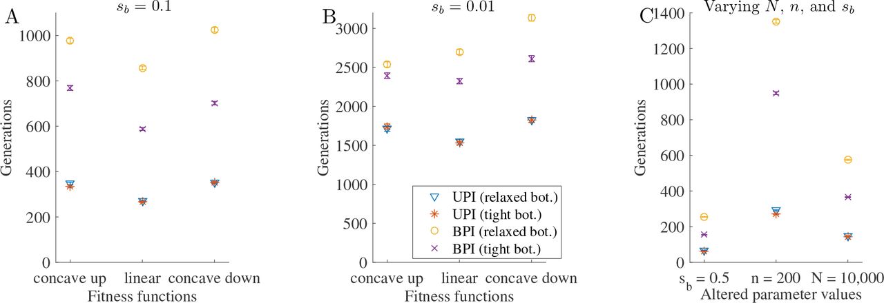
Each plot shows the number of generations to accumulate a beneficial substitution (number of generations before each cytoplasmic genome carries at least γ substitutions—where γ = 5—divided by the mean substitutions per genome in that generation). Parameter values for A—B: N = 1000, n = 50, μb = 10−8, and b = 25 (relaxed transmission bottleneck) or b =5 (tight transmission bottleneck). A. Selection coefficient of 0.1. B. Selection coefficient of 0.01. Parameter values for C (unless otherwise stated on the x-axis): N = 1000, n = 50, μb = 10−8, sb = 0.1, a linear fitness function for beneficial substitutions, and b = n/2 (relaxed transmission bottleneck) or b = n/10 (tight transmission bottleneck). Error bars are standard error of the mean.

To calculate the genetic hitchhiking index(ϕ), we compare the number of generations separating beneficial and deleterious sweeps to the number of generations we expect if the two events are uncorrelated. We examine all beneficial sweeps except those involving genomes with > 5 beneficial substitutions (to maintain consistency between the different fitness functions). We map each beneficial sweep to a single deleterious sweep but do not limit the number of times a single deleterious sweep can be mapped to (e.g. B and C). The expected separation between beneficial and deleterious sweeps for this hypothetical example is shown at the top of the figure. See below for details of how the index is calculated. A. When beneficial sweeps are closely followed by deleterious sweeps, ϕ < 1 and we infer that genetic hitchhiking has occurred. B. When the mean of the number of generations separating beneficial and deleterious sweeps are as expected, ϕ ≈ 1 and we infer that the beneficial sweep does not affect the deleterious sweep. C. When deleterious sweeps follow beneficial sweeps later than expected, ϕ > 1 and we infer that genetic hitchhiking is suppressed. D. When a beneficial sweep is followed by a deleterious sweep, we call it a “paired” sweep. In some instances, the simulation terminates before a deleterious sweep can follow a beneficial sweep (an “unpaired” sweep; e.g. the last beneficial sweep in D). For unpaired sweeps, we add the number of generations separating the beneficial sweep and the end of the simulation. To calculate the mean generations separating the sweeps, however, we only divide by the number of paired sweeps. Thus, the equation for the index is  . np is the total number of paired sweeps, gd(i) is the generation in which the ith paired deleterious sweep occurred, and gb(i) is the generation in which the ith paired beneficial sweep occurred. nu is the total number of unpaired sweeps, gt is the number of generations in each run (10000), and gd(κ) is the generation in which the jth unpaired beneficial sweep occurred. E[s] is the expected separation in generations and given by
  , where d(κ) is the number of deleterious sweep occurred in the κth simulation, gd(κ) is the generation at which the d(κ)th deleterious sweep occurred in the κth simulation, and r is the number of runs for each set of parameter values (500). We subtract 1 because the deleterious sweeps can occur in the same generation as the beneficial sweep.

Parameters: N = 1000, n = 50, μb = 10−9, μd = 10−7, and b = 25 (relaxed transmission bottleneck) or b = 5 (tight transmission bottleneck). A shows a selection coefficient of 0.1 while B shows a selection coefficient of 0.01. The plots show the overall level of genetic hitchhiking in each population, measured by our genetic hitchhiking index (see Fig. S2 for details). When ϕ < 1, it indicates the presence of genetic hitchhiking. Error bars are ± standard error of the mean. Note that this figure depicts a beneficial mutation rate 10 times smaller than shown in Fig. 5 (μb = 10−9 versus μb = 10 −8).

Parameters: N = 1000, n = 50, μd = 10−7, and b = 25 (relaxed transmission bottleneck) or b = 5 (tight transmission bottleneck). Panels A and B show selection coefficients of sb = sd = 0.01, while panels C and D show selection coefficients of sb = sd = 0.1. For panels A and C, the beneficial mutation rate is μb = 10−8, while for panels B and D the beneficial mutation rate is μb = 10−9. In all cases, uniparental inheritance has a higher ratio of beneficial to deleterious substitutions than biparental inheritance. Error bars are ± standard error of the mean. See Fig. 7 legend for details of how we calculate the ratio of beneficial to deleterious substitutions.
Benchmarking the genetic hitchhiking index using randomly simulated data
Note. — Parameters: N = 1000, n = 50. ϕ ± sd shows the genetic hitchhiking index for randomly simulated datasets ± standard deviation. For each set of parameter values, we determined the expected distance between beneficial and deleterious sweeps. (The expected distance separating beneficial sweeps is  , where nb(i) is the number of beneficial sweeps we considered in the ith simulation, gb(i) is the generation at which the nb(i)th beneficial sweep occurred in the ith simulation, and r is thp number of runs for each set of parameter values (500). The expected distance separating deleterious sweeps is
  , where nd(i) is the number of deleterious sweeps we considered in the ith simulation, gd(i) is the generation at which the nd(i)th deleterious sweep occurred in the ith simulation, and r is the number of runs for each set of parameter values.) We used these expected values to generate 500 randomly simulated runs, and for each one, used binomial sampling to generate a random number of beneficial and deleterious sweeps. (The number of beneficial sweeps is given by the random variable
  and the number of deleterious sweeps by the random variable
  , where i is the number of the simulated run (out of 500). To obtain
  and
and  , we used the R function rbinom with parameters n = 1, size = 10000, and prob = 1/E[dd] for beneficial sweeps or prob = 1/E[dd] for deleterious sweeps.) For each run, we uniformly sampled
  beneficial and
  deleterious sweeps over 10,000 generations to get the locations of our random beneficial and deleterious sweeps. We then calculated ϕ in the same way as our model-generated data (Fig. S2). For each set of parameter values, we repeated this process 100 times, giving us 100 estimates of ϕ. The fifth column shows the mean and standard deviation of these 100 estimates. As can be seen, when beneficial and deleterious sweeps are uncorrelated, ϕ ≈ 1.
REFERENCES
- [1].↵
- [2].↵
- [3].↵
- [4].↵
- [5].↵
- [6].↵
- [7].↵
- [8].↵
- [9].↵
- [10].↵
- [11].↵
- [12].
- [13].↵
- [14].↵
- [15].↵
- [16].↵
- [17].↵
- [18].↵
- [19].↵
- [20].↵
- [21].↵
- [22].↵
- [23].↵
- [24].↵
- [25].↵
- [26].↵
- [27].↵
- [28].↵
- [29].↵
- [30].↵
- [31].↵
- [32].↵
- [33].↵
- [34].↵
- [35].
- [36].↵
- [37].↵
- [38].↵
- [39].↵
- [40].↵
- [41].↵
- [42].↵
- [43].↵
- [44].↵
- [45].↵
- [46].
- [47].↵
- [48].↵
- [49].↵
- [50].↵
- [51].
- [52].↵
- [53].↵
- [54].↵
- [55].↵
- [56].↵
- [57].↵
- [58].↵
- [59].↵
References
- [1].
- [2].
- [3].
- [4].
- [5].


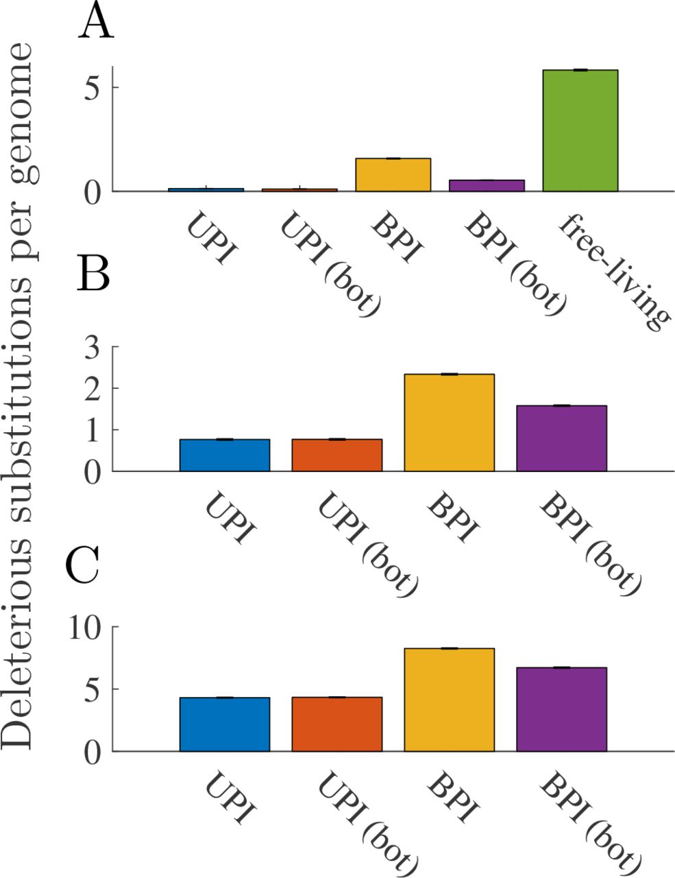
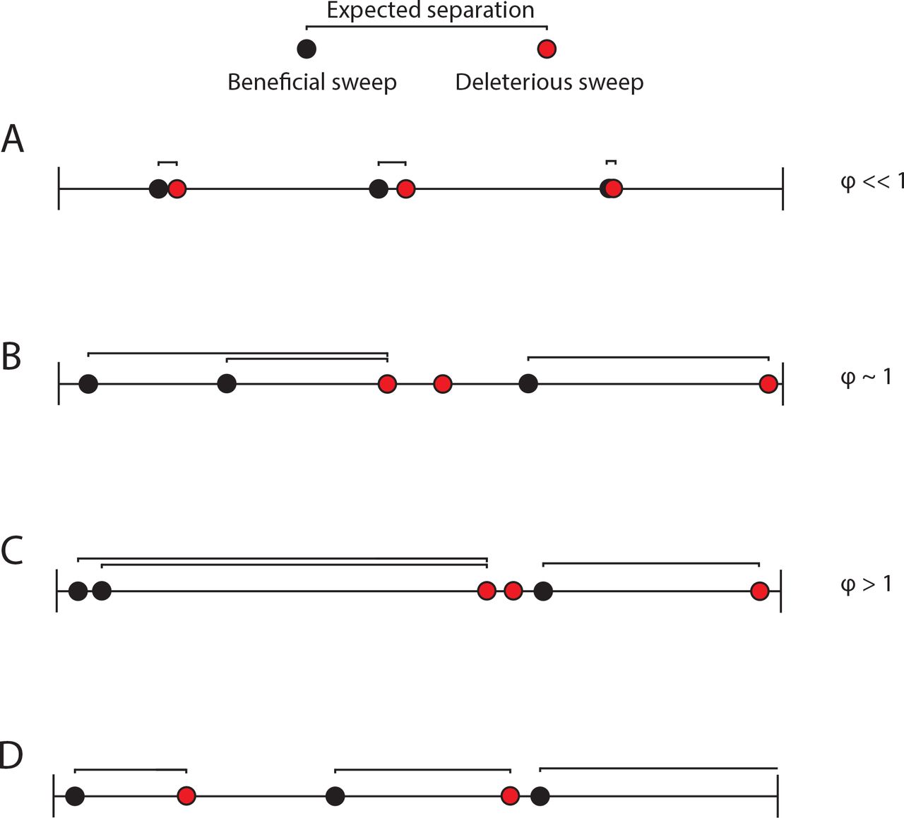