

Abstract
Our work addresses two key challenges, one biological and one methodological. First, we aim to understand how proliferation and cellular migration rates in the intestinal epithelium are related under healthy, damaged (Ara-C treated) and recovering conditions, and how these relations can be used to identify mechanisms of repair and regeneration. We analyse new data, presented in more detail in a companion paper, in which BrdU/IdU cell-labelling experiments were performed under these respective conditions. Second, in considering how to more rigorously process these data and interpret them using mathematical models, we develop a probabilistic, hierarchical framework. This framework provides a best-practice approach for systematically modelling and understanding the uncertainties that can otherwise undermine drawing reliable conclusions - uncertainties in experimental measurement and treatment, difficult-to-compare mathematical models of underlying mechanisms, and unknown or unobserved parameters. Both discrete and continuous process models are considered and related via hierarchical conditional probability assumptions. This allows the incorporation of features of both continuum tissue models and discrete cellular models. We perform model checks on both in-sample and out-of-sample datasets and use these checks to illustrate how to test possible model improvements and assess the robustness of our conclusions. This allows us to consider - and ultimately decide against - the need to retain finite-cell-size effects to explain a small misfit appearing in one set of long-time, out-of-sample predictions. Our approach leads us to conclude, for the present set of experiments, that a primarily proliferation-driven model is adequate for predictions over most time-scales. We describe each stage of our framework in detail, and hope that the present work may also serve as a guide for other applications of the hierarchical approach to problems in computational biology.
Introduction
Motivation
The intestinal epithelium provides crucial barrier, transport and homeostatic functions. These requirements lead it to undergo constant repair and regeneration, and dysfunctions can result in pathologies such as tumorigenesis (Wright and Alison 1984; Radtke and Clevers 2005; Reuss 2010; van der Flier and Clevers 2009; Turner 2009; Marchiando, Graham, and Turner 2010; Barker 2014). While much work has been carried out on estimating the rate parameters in the intestine and other epithelia (Wright and Alison 1984; Kaur and Potten 1986a; Kaur and Potten 1986b; Tsubouchi 1983), attempts to interpret these experimental data using mechanistic modelling remain inconclusive (see e.g. Dunn, Näthke, and Osborne 2013; Meineke, Potten, and Loeffler 2001; Loeffler et al. 1986; Loeffler et al. 1988). A key issue in drawing reliable conclusions is the lack of consistent and reproducible frameworks for comparing models representing conjectured biological mechanisms, both to each other and to experimental data.
This challenge goes in both directions: using experimental data (taken to be ‘true’) to parameterise and test mathematical or computational formalisations of mechanistic theories, and using these models (taken to be ‘true’) to predict, interpret and question experimental results. Both experimental measurements and mathematical models are subject to uncertainty, and we hence need systematic ways of quantifying these uncertainties and attributing them to the appropriate sources. Furthermore, establishing a common framework for analysing experimental results, formulating mechanistic models and generating new predictions has many potential advantages for enabling interdisciplinary teams to communicate in a common language and efficiently discover and follow promising directions as and when they arise.
Approach
We address the above issues by developing a best-practice hierarchical Bayesian framework for combining measurements, models and inference procedures, and applying it to a tractable set of experiments targeting mechanisms of repair and regeneration in the intestinal epithelium. These experiments were performed ourselves and are presented in more detail in (Parker et al. 2016). The aim of these experiments was to identify how proliferation rates, tissue growth and cellular migration rates are related under healthy, damaged (Ara-C treated) and recovering conditions, and how these relations can be used to identify mechanisms of repair and regeneration.
A notable feature of the Bayesian approach to probabilistic modelling is that all sources of uncertainty are represented via probability distributions, regardless of the source of uncertainty (e.g. physical or epistemic) (Bernardo and Smith 2009; Gelman et al. 2013; Tarantola 2005). We will adopt this perspective here, and thus we consider both observations and parameters to be random variables. Within a modelling or theoretical context, uncertainty may be associated with (at least): parameters within a mechanistic model of a biological or physical process, the mechanistic model of the process itself and the measurements of the underlying process. This leads to the existence (at least in principle) of a full joint probability distribution for observable, unobservable/unobserved variables, parameters and data.
Another key feature of the Bayesian perspective, of particular interest here, is that it provides a natural way of decomposing such full joint models in a hierarchical manner, e.g. by separating out processes occuring on different scales and at different analysis stages. A given set of hierarchical assumptions corresponds to assuming a factorisation of the full joint distribution mentioned above, and gives a more interpretable and tractable starting point.
Our overall factorisation follows that described by (Berliner 1996; Tarantola 2005; Cressie and Wikle 2011; Wikle 2015). This comprises: a ‘measurement model’, which defines the observable (sample) features to be considered reproducible and to what precision they are reproducible (the measurement scale); an underlying ‘process’ model, which captures the key mechanistic hypotheses of spatiotemporal evolution, and a prior parameter model which defines a broad class of a priori acceptable possible parameter values.
This hierarchical approach is being increasingly adopted - especially in areas such as environmental and geophysical science (Berliner 2003; Wikle 2003), ecological modelling (Cressie et al. 2009; Ogle 2009), as well as in Bayesian statistical modelling and inverse problems more generally (Berliner 1996; Tarantola 2005; Cressie and Wikle 2011; Wikle 2015; see also Gelman et al. 2013; Blei 2014). In our view, however, many of the advantages of hierarchical Bayesian modelling remain under-appreciated and it offers many opportunities for formulating more unified frameworks for model-data and model-model comparison. Furthermore, we note that a similar hierarchical approach has recently received significant development in the context of the non-Bayesian ‘extended-likelihood’ statistical modelling framework utilising random-effects models (see for example Pawitan 2001; Pawitan and Lee 2016; Lee, Nelder, and Pawitan 2006). Thus, in our view, many of the benefits of the present approach can be attributed to its hierarchical aspect in particular (Cressie and Wikle 2011 also emphasise this point).
As illustration of some of the modelling benefits of the hierarchical approach, we show how both discrete and continuous process models can be derived and related using the hierarchical perspective. This thus provides a clear, unified approach for understanding different - yet related - models and derivations, and for embedding models within a data-driven parameter estimation framework. The hierarchical perspective also provides a natural guide to exploring robustness to model closure assumptions, investigating model misfit and checking for invariance of proposed mechanisms under in/out-of-sample and treated/untreated conditions. These considerations are necessary since, despite the utility of statistical methods for obtaining parameter estimates and model predictions based on an assumed-to-be-true model and assumed-to-be-true datasets, it is also well-known that ‘all models are wrong’ (Box 1976) and that purely statistical modelling is generally inadequate for drawing causal conclusions without additional assumptions (Pearl 2009a; Pearl 2009b). We adopt a straightforward conditional/hierarchical interpretation of causal modelling (see Dawid 2010a; Dawid 2010b for clear overviews) and emphasise the distinct roles of (Bayesian) predictive distributions vs. parameter distributions for model checking and the assessment of evidence, respectively (see Box 1976; Box 1980; Evans 2015; Gelman and Shalizi 2013; Gelman et al. 2013 for clear discussion of these distinctions).
Conclusions
For predictions over moderate time-scales a primarily proliferation-driven model appears adequate as a sound starting point. Our framework offers a systematic, hierchical modelling perspective for exploring and testing possible improvements, and using Bayesian inference for estimating parameters and generating model predictions. Our interdisciplinary approach, mixing new experimental work with mathematical and computational modelling, enables us to more reliably consider and test various hypotheses than would likely be obtained using only one or the other approach.
Structure
Our article is structured as follows. We first outline the experimental procedures (which are also described in more detail in Parker et al. 2016). We then show in detail how we build up our mathematical model, beginning from the data available, the resolution of the measurement process and a hypothesised underyling ‘true’ or ideal population from which samples are assumed to be drawn. We then consider both discrete and continuous representations of the spatiotemporal evolution of the underlying population, their relation to each other and some of the strengths and weaknesses of different representations. We then present the methods and results for our baseline and Ara-C-treated experiments, using our modelling and exploratory data analysis to interpret them. Each stage is described in quite some detail in order to demonstrate how the present framework may be adapted and used for other problems of computational biology more generally.
Materials and methods I: Experimental treatments
Homeostasis mouse model
To obtain estimates of intestinal epithelial proliferation and migration rates under normal, homeostatic conditions in healthy mice, we used standard methods of proliferative cell labelling and tracing (Wright and Alison 1984; Kaur and Potten 1986a; Kaur and Potten 1986b; Tsubouchi 1983; see Parker et al. 2016 for full details). Actively proliferating cells in the intestinal crypts were labelled by single injection of the thymine analogue 5-bromo-2-deoxyuridine (BrdU) and labelled cells detected by immunostaining of intestinal sections collected from different individuals over time. Migration of labelled cells traced from the base of crypts to villus tips was monitored over the course of 96 hours (5760 min).
Blocked-proliferation mouse model
To assess the effects of proliferation inhibition on crypt/villus migration, migrating and proliferating epithelial cells were monitored by double labelling with two thymine analogues (BrdU and IdU), administered sequentially a number of hours apart and subsequently distinguished by specific immunostaining in longitudinal sections of small intestine. Following initial IdU labelling of proliferating cells at t= -17h (-1020 min, relative to Ara-C treatment), mice were then treated with cytosine arabinoside (Ara-C) at 250 mg/kg body weight, a dose reported to inhibit proliferation without causing major crypt cell atrophy (see Parker et al. 2016 and references therein for full details). Tissues were collected over 24 hours, with BrdU administered one hour prior to collection to check for residual proliferation. Successful inhibition of proliferation following treatment with Ara-C was confirmed by an absence of BrdU (S-phase) and phospho-Histone H3 (pH3) staining (M-phase) in longitudinal sections of small intestine (again, see Parker et al. 2016 for full details).
Recovering-proliferation mouse model
The above Ara-C treatment effect was observed to last for at least 10h (600 min). Cell proliferation resumed to near normal levels in samples obtained 18h (1080 min) post-Ara-C treatment.
Materials and methods II: Mathematical framework
Overview
Here we build up a hierarchical probability model on the basis of conditional probability assumptions which are used to factor out a measurement model, a mechanistic model and a parameter model. We will interpret and visualise this hierarchical model in an operational manner i.e. as defining various ensembles (e.g. prior and/or posterior parameter and/or predictive ensembles) consisting of sequences of draws from the component distributions of the full product (see e.g. Hartig et al. 2011; Wilkinson 2011; Gutmann and Corander 2015 for discussion of simulation-based interpretations of Bayesian models). We first discuss the model components, after which we summarise the overall model structure and computational implementation of the model in the ‘Computational methods’ section that follows.
Measurement model
Observable features and underlying population
Our aim is to connect experimental measurements to mechanistic models. Rather than begin from mechanistic hypotheses before considering the connection to available data, here we explicitly begin by thinking about the available data, how it is obtained and what the key features of interest are. These key features will then be considered to define an ideal ‘underlying population’ from which samples are considered to be drawn or to which they are to be compared. This means that we begin the construction of our hierarchical model in a ‘top-down’ (data-to-parameter) manner.
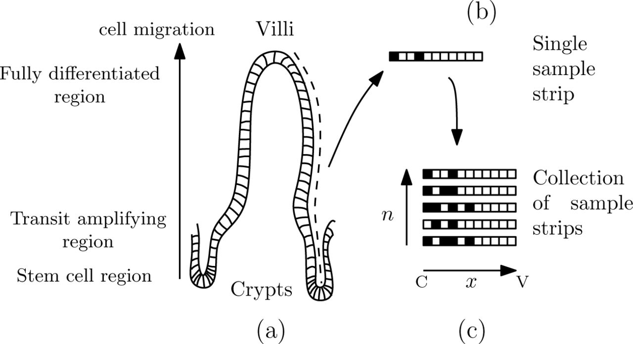
With reference to Fig (1), we consider a collection of one-dimensional ‘strips’ of cells. These strips run from the base of the crypt to the tip of the villus, i.e. along the so-called ‘crypt-villus’ axis, and correspond to how strips are collected experimentally. Each of these strips can be considered as arising from a ‘measurement’ from the (hypothesised) ‘true underlying population’ of such strips. Equivalently, the underlying population can be considered to define the ‘reference frame’ with respect to which the (finite) samples are analysed (and without which samples have little meaning). Measurements can be given a spatial location index i and a time label t; we will represent these by a single index parameter s := (i, t), when notationally convenient. In our case we assume each strip is independent of the others as, in general, strips are taken from different crypt-villus units and/or animals after ‘identical preparation’.

The (a) intestinal epithelium, (b) individual measurements as strips of cells and (c) collection of strips, where ‘C’ and ‘V’ indicated ‘crypt’ and ‘villus’ respectively.
Thus we do not ever directly possess, for example, measurements of a particular crypt with dimensions given in terms of a certain number of strips, though we will distinguish between the underlying population of strips (full ensemble) and a particular sample of strips at hand. Characterising a ‘typical’ reference crypt-villus unit by the two vectors (L, n), where L is the vector of labelled fractions at each grid point and n is the vector of number of samples at each grid point, gives a useful reduction of the (spatially) two-dimensional dynamics to a (spatially) one-dimensional problem. In general the dynamics of strips in a given crypt may be affected by those in the same crypt but we will not consider this additional complexity at present.
Given our choice of key observable as y, the vector of counts of labelled cells at each grid point, and key ‘ideal characteristics’ of comparison (L, n), we will assume that all s are exchangeable (see Bernardo and Smith 2009; Gelman et al. 2013 for a formal definition and further discussion) conditional on (L, n). Satisfying this exchangebility condition implies the existence of a Bayesian probability model and is, in essence, a statistical reduction/symmetry assumption (see Bernardo and Smith 2009; Gelman et al. 2013 for more). Thus we will assume the existence of some p(y|L, n), which links observables to an underlying population. Note that we will consider different experimental treatment conditions E, but the measurement component will be taken to be independent of E - i.e. treatment will be taken to affect the underlying process parameters only (this is discussed in more detail in ‘Summary of hierarchical structure’).
A slight strenghtening (see Bernardo and Smith 2009; Gelman et al. 2013) of the general exchangeability assumption (which leads to a pure existence theorem) to the independence assumption discussed above leads to a particular model for the number of labelled cells ys drawn in a collection of ns cells at grid location s. This corresponds to a binomial distribution ℬ with probability Ls at each grid location, giving the factorisation

Note that this certainly does not imply that the underlying parameters L(i, t) are independent, rather that if the true parameters are known at each location then observations can be made independently at those locations (as discussed in the above).
Likelihood and normal approximation
The above justifies a measurement component p(y|L, n) of the full sampling model for the probability of a set of observed labelled cells y in samples of sizes n given the vector of modelled underlying labelled fractions L. This also gives a likelihood function ℒ for this measurement model, which is proportional to the probability given by the sampling model evaluated for the observed data and considered as a function of L, i.e.

It is also helpful to note that, for each s, if ns is sufficiently large and Ls is not too close to 0 or 1 (e.g. nsLs and ns(1 − Ls) > 5 is typical) then we may replace the binomial distributions ℬ(ns, Ls) by their normal approximations  . In this case we can use, denoting the set of all measured labelled fractions through the (useful, but slightly non-standard) notation y/n := (y1/n1, …, yS/nS),
 where the standard deviations are given by
  . Since these standard Ls in addition to the ns we cannot drop them from the likelihood function. This normal approximation formulation is useful for the construction of approximate uncertainty intervals and, as we illustrate later, checking model misfit.
Process models
Discrete, measurement-grid-level process model
Here we first consider a formulation of our governing ‘process’ equations as a discrete probabilistic model. This captures the evolution of the (population) ‘measurement’ probability (labelled fraction) at the scale of the measurement grid. We will later consider an underlying continuous approximation to this model which discards some arbitrary details of the discrete model and so, though an approximation, it may in another sense be more generally applicable. It introduces a finer, continuous, spatial scale than the discrete measurement grid. The relationships between discrete and continuous representations motivates various possible modifications to, and interpretations of, our process equations, which we discuss later.
Again with reference to Fig (1), we consider a collection of one-dimensional ‘strips’ of cells. For our probabilistic discrete model, we use li ∈ {0, 1} as an indicator variable denoting the occupancy status of site i of a given strip. The full state of this strip is then given by the vector l = (l0, l1, …lS−1). We first seek a description of the probabilistic dynamics in terms of a discrete-time Markov chain for the probability distribution of the full state p(l, t) (see e.g. Van Kampen 1992; Wilkinson 2011). Though we will begin from an explicit joint distribution for the full state we will show this reduces here to a description in terms of the set of ‘single-site’ probability distributions p(li, t) for each site i.
For the following derivations it is helpful to adopt an explict notation. Thus we will denote the probabilities of occupancy and vacancy at site i at time t by p(li(t) = 1) and p(li(t) = 0) respectively, and note that since p(li(t) = 1) + p(li(t) = 0) = 1 we only need to consider the probability of occupancy to fully characterise the distribution p(li(t)) (and, of course, similar properties hold for conditional distributions - see below).
The equation of evolution for this probability can be conveniently derived by considering conservation of probability in terms of probability fluxes in and out, giving, to first order in Δt

The first term on the right represents a net ‘influx of occupancy probability’ due to a single division event somewhere at site j < i, each division event having a probability given by kjΔt. This flux leads to the value of the state variable li(t) = 0 being replaced, at the next time step, by the value of li−1(t) = 1. The second term similarly represents a net ‘outflux of occupancy probability’ due to a division event somewhere at site j < i.
We can further simplify this due to the binary nature of the occupancy state. To do this, note that since li(t) = 0 and li(t) = 1 partition the event space of li(t), we have
 and similarly, since li−1(t) = 0 and li−1(t) = 1 partition the event space of li−1(t), we have

This leads to the above-mentioned simplification in terms of only single-site probability distributions

Underlying continuous model
Here we introduce a smooth parameter field of ‘true’ labelled fractions L(x, t), now defined over a continuous space-time domain, and which corresponds to a further idealisation of the ‘underlying population’ from which we envisage the strips are sampled. The smoothness assumption, while not strictly necessary, means we will be able to give an interpretation of some model properties in terms of local derivatives; it also makes future comparisons with off-lattice and/or continuum models (see Maclaren et al. 2015 for a review of various model types) more directly possible, and reduces arbitrary dependence on discrete grid features.
The position x is taken to be a continuous coordinate passing through the discrete cell indices, e.g. x = 0 denotes the coordinate of the cell labelled ‘0’ (base of the crypt), while x = 0.5 is the location halfway between the cell labelled ‘0’ and that labelled 1’. We will indicate sample locations consisting of space-time pairs by s = (xs, ts). Then, for sample locations (i, t) corresponding to cell indices and arbitrary times, we match the discrete model and continuous model using
 i.e. L(i, t) serves as the parameter for a single measurement modelled as a Bernoulli trial at that sample location (as in the above measurement model section).
Now, we consider how the discrete dynamics of p(li(t) = 1) can be transferred to the continuous L(x, t) dynamics. In particular, since L(x, t) is a smooth function, we can make the correspondence
 where Δx = i − (i − 1) = 1 is the normalised cell length and we have also conditioned on knowledge of the spatial derivatives at
  etc. Here the continuous spatial field can be considered to be interpolating between - i.e.internal to - points of the discrete grid, making use of local derivative information. Substituting the above Taylor series, and similar expressions, into the discrete Markov equation (7) leads to
 where we have, for completeness, also retained higher order terms in Δt for the continuous model. We have also similarly assumed the existence of smooth functions k(x, t) and υ(x, t) that satisfy the discrete relations

We will assume k(x, t) = k(x), υ(x, t) = υ(x) and υ(0) = 0 in what follows.
Now we obtain closure for the continuous model by keeping only the lowest order terms in both time and space, and further asserting that the equation structure obtained should hold for all (continuous) x and not just (discrete) i (this can also be motivated by an assumption of grid translation invariance). This gives the advection equation
 with
with

The above partial differential equation (PDE) has a straightforward continuum interpretation as the advection of a tracer in an incompressible fluid field with a source, and is sometimes referred to in this context as the ‘colour equation’ (LeVeque 2002). We will take advantage of this in analysing model properties. Furthermore, it is straightforward to show that incorporating cell death, with discrete rates di, leads to the same equations with k replaced by k − d, where d(x, t) is defined similarly to k(x, t), and hence we will interpret k in the above as the net cell production rate.
Higher-order spatial effects
Our smooth interpolation of the discrete set of equations into a continuous equation is a process of ‘continualisation’ - the reverse process of discretising a continuous equation to obtain a numerical scheme (see e.g. Askes and Metrikine 2005; LeVeque 2002 Section 8.6 for similar ideas). Thus we might expect that a better continuum approximation could be obtained by retaining higher-order spatial derivatives and hence finite-cell-size effects.
As one possible model improvement and/or perturbation, here we reconsider the continuous approximation of our discrete Markov equation. In particular we consider retaining the higher-order spatial derivative. This naturally gives rise to a Fokker-Planck equation containing a diffusion term (Van Kampen 1992). Equations of this (and similar) form have been derived before, also based on continuous approximations to discrete master equations (e.g. Baker, Yates, and Erban 2010; Hywood, Hackett-Jones, and Landman 2013; while Fozard et al. 2010; Murray et al. 2009 also contain similar ideas; Maclaren et al. 2015 give additional references).
Reconsidering the expansion in (10), we will again neglect all terms of order Δt; however we now retain the next order spatial derivative leading to
 where D(x) = (1/2)Δxυ(x).
Here retaining the second spatial derivative amounts to accounting for spatial effects due to finite cell sizes. Though we will first evaluate our original ‘zeroth-order’ (advection) model against our data, we will later examine the extent to which higher-order spatial terms such as those considered here may account for any misfits.
Parameter model
Within a Bayesian approach the choice of prior distribution is as important a part of model construction as the choice of sampling model (measurement and process components) and can be used to include relevant scientific information and constrain or ‘regularise’ the physical and mathematical characteristics of solutions (Gelman et al. 2013 provides an applied account of this approach while Gelman and Shalizi (2013) presents a more philosophical perspective). In particular we can constrain the variability of the (here) spatially varying parameter field a priori to help avoid unphysical solutions, as well as vary these prior assumptions to explore the solution dependence on parameter variability.
We represent possible proliferation profiles, varying with cell locations, as realisations from a prior given in terms of a discretised random field (a random vector) k of length m, modelled as a multivariate Gaussian  with joint distribution

The properties of this distribution are determined by its mean vector μ and covariance matrix C. Furthermore, we decompose the latter into a standard deviation matrix given by the outer (tensor) product of the standard deviation vector for each variable, S = σσT, and correlation matrix R. These multiply element-wise to give Cij = SijRij summation).
Another common, equivalent, representation is C = DRD where D is a diagonal matrix with diagonal entries Dii = σi. Decomposing the covariance into these separate parts makes clearer how we can control the smoothness and magnitude of variations via off-diagonal and diagonal terms, respectively, in addition to the mean response.
We will assume that the correlation matrix R is obtained from the squared-exponential (Gaussian) correlation function  where lc is a parameter controlling the characteristic length-scale of the correlations - e.g. the scale over which the correlation function decays to 1/e - and x and x′ are two spatial locations. This allows us to control the ‘smoothness’ of the realisations from the prior, in the sense that as l is increased the values at x and x′ tend to be more similar. We generate the matrix R by evaluating this correlation function at the locations of a discretised grid of proliferation activity (here chosen to be coarser than the cell index grid), and lc can then also be interpreted as a ‘parameter correlation length’, a measure number of the parameters over which the correlations decay. We will typically consider correlation lengths of 1-2 parameters.
In line with our approach of providing a ‘simulation’ or ‘sampling-based’ interpretation of a given model structure, it is typically most informative to visualise realisations of the whole function from the resulting prior rather than simply give the individual parameters/matrices separately (Tarantola 2005 discusses this in more detail). These will be discussed and displayed in more detail in the Results section below.
Summary of hierarchical structure
Here we show how to piece together the above model components.
We begin from a full joint distribution for a given experimental treatment E and known sample size vector n, decomposing it according to

This hierarchical factorisation makes clear the conditional independence closure assumptions which separate the dependencies of the various levels, i.e. p(y|L, k, n, E) = p(y|L, n), p(L|k, n, E) = p(L|k) and p(k|n, E) = p(k|E). Furthermore, a ‘causal’ - structural invariance - assumption is made in assuming that the experimental treatment condition only affects the process parameter k but not the structure of the measurement or process models (see e.g Pearl 2009a; Pearl 2009b; Dawid 1979; Dawid 2010a; Dawid 2010b; Woodward 2003; Woodward 1997; Spirtes, Glymour, and Scheines 2000 for discussions of causal modelling and structural invariance).
The above factorisation can, and will, be checked to some extent in what follows. In particular, we distinguish working ‘within’ the model - e.g. parameter estimation assuming the model and factorisation is valid - and working ‘outside’ the model e.g. checking the validity of the model structural assumptions themselves (see Gelman and Shalizi 2013; Gelman et al. 2013; Evans 2015 for relevant discussion of the distinction). From now on we will suppress the sample size n as it will be taken to be fixed and known, and will also in general suppress the conditioning on E (keeping in mind that it only affects k).
As implicit in the model derivations above, we use a deterministic expression of conservation of probability (as is typical for Markov/master/Fokker-Planck equations; see Van Kampen 1992) for our process model and so the relationship between any set of process parameters k and the output process variable L, p(L|k), can be (formally) taken to be a Dirac delta function centred on the relationship described by the ‘true’ model (e.g. Tarantola 2005). It suffices for our purposes to simply replace all functional dependencies on the process variable above with a dependence on the process parameters.
Computational methods
Interpretation and implementation of model updating and inference
The above provides a ‘predictive’ or ‘generative’ probabilistic model. Thus, given an initial specification (‘prior parameter model’ and ‘forward/process model’) of each of these parts we can construct ‘prior predictions’ according to (see e.g. Gelman et al. 2013; Maclaren et al. 2015)
 where we have made use of the aforementioned deterministic link between a given sample of process parameters and the output process variable, L = f(k). Here we follow statistical standard notation where ∼ denotes ‘distributed as’, or more relevantly, ‘samples drawn according to’.
If, or when, new data y0 become available one can update the parameters of the model to improve the predictive model and hence pass to a ‘posterior predictive’ model (again, see e.g. Gelman et al. 2013)
 where we have introduced the conditional probability closure assumption p(y|f(k), y0) = p(y|f(k)). This closure assumption may be interpreted as maintaining our same mechanistic model despite new observations, and thus again connects well with current theories of causality as based on ideas of structural invariance (Pearl 2009a; Pearl 2009b; Dawid 1979; Dawid 2010a; Dawid 2010b; Woodward 2003; Woodward 1997; Spirtes, Glymour, and Scheines 2000).
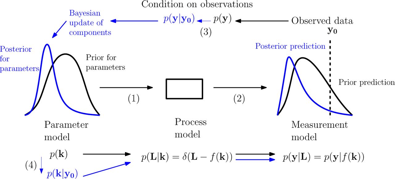
The logical flow is depicted in Fig (2). If we consider proceeding from the ‘lowest’ level to the ‘highest’ level, then each lower level draw gives a parameter (or set of parameters) to be plugged into the higher level distributions and generate further draws, ultimately producing predictions to be compared to actual data. Distributions are updated in the ‘reverse’ manner by conditioning at the highest level and propagating the implications of this back down the hierarchy. The conditional independence probability statements separating the levels may be considered as testable modelling ‘closure’ assumptions.

Illustration of the Bayesian predictive and parameter inference processes. Following the arrows (1) to (2) we move from a prior parameter model (left, black) to associated predictive distribution (right, black) via the process and measurement models. Following the arrows (3) to (4) we condition on observed data to obtain a posterior parameter model (left, blue) and associated predictive distribution (right, blue). Our structural assumptions mean that the information gained is represented in updates of the parameter model while the process and measurement models maintain the same form. Modified from (Maclaren et al. 2015), which was based on (Iglesias and Stuart 2014).
To implement the updating from prior to posterior parameter distributions, given measurements, we used Monte Carlo Markov Chain (MCMC) sampling (see Robert and Casella 2013 for a comprehensive reference). In particular, we used the (open source) Python package emcee (http://dan.iel.fm/emcee/) which implements an ‘affine-invariant ensemble sampler’ MCMC algorithm and has been applied in particular to astrophysics problems (see Foreman-Mackey et al. 2012 for details). Given samples from the resulting prior and posterior parameter distributions, respectively, prior and posterior predictive distributions were obtained by forward simulation as described above. Note that each candidate proliferation rate vector k is connected to the measurements y via the latent vector L; since this step is deterministic, however, no additional sampling steps are required for the process model component.
Interpretation of statistical evidence
As discussed above, our interpretation of mechanism/causality is as structural invariance under different scenarios. Even given this, we still need to provide an interpretation of the ‘evidence’ that a set of measurements provides about parameter values within a fixed model structure. There is still a surprising amount of controversy and debate about fundamental principles and definitions of (statistical) evidence, however (see e.g. Mayo 2014; Evans 2014).
Following our conditional modelling approach, here we adopt the simple - yet generally applicable - principle of evidence based on conditional probability: if we observe b and p(a|b) > p(a) then we have evidence for a. A ‘gold-standard’ theory of statistical evidence starting from this premise has been developed and defended recently by Evans in a series of papers (summarised in Evans 2015). Besides simplicity, a nice feature of this approach that we will use is that it can be applied both to prior and posterior predictive distribution comparisons such as  , as well as to prior and posterior parameter distribution comparisons such as
  . In practice, we emphasise the visual comparison of various prior and posterior distributions (Tarantola 2005 advocates a similar “movie strategy” for the interpretation of statistical evidence and inference procedures).
Differential equation solvers
In all sections other than the later section in which we include higher-order spatial effects, we solve the differential equation model using the PyCLAW (Ketcheson et al. 2012; Mandli, Ketcheson, and others 2014) Python interface to the CLAWPACK (Clawpack Development Team 2014) set of solvers for hyperbolic PDEs. We adapted a Riemann solver for the colour equation available from the Riemann solver repository (https://github.com/clawpack/riemann). For testing the inclusion of higher-order spatial effects (thus changing the class of our equations from hyperbolic to parabolic) we used the Python finite-volume solver FiPy (Guyer, Wheeler, and Warren 2009).
Jupyter Notebook and summary of main packages used
Our code is available in the form of a Jupyter (previosuly IPython) Notebook (http://ipython.org/notebook.html) in the Supplementary Information. To run these we used the Anaconda distribution of Python (https://store.continuum.io/cshop/anaconda) which is a (free) distribution bundling a number of scientific Python tools. Any additional Python packages and instructions which may be required are listed at the beginning of our Jupyter Notebook.
Results
Parameter inference under homeostatic (healthy) conditions
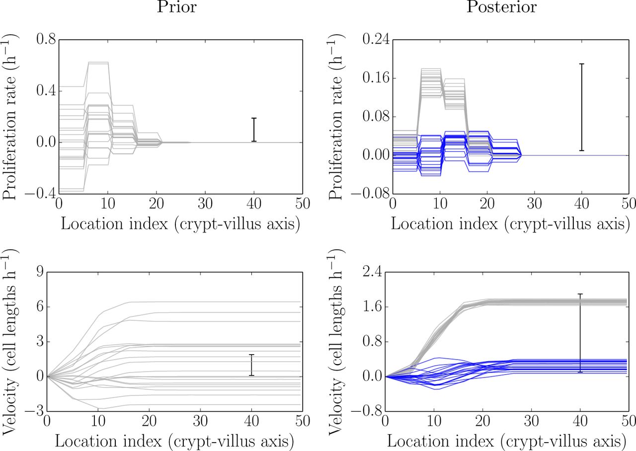
Fig (3) illustrates the process of updating from (realisations from) the prior (pre-data) distributions of the proliferation and velocity fields to (realisations from) their posterior (post-data) distributions. The left-hand side of the figure shows simulations from the prior distribution for proliferation field (top) and realisations from the induced distribution for the velocity field (bottom), respectively. The right-hand side shows the corresponding simulations after the prior parameter distribution has been updated to a posterior parameter distribution. The prior-to-posterior parameter estimation was carried out using the MCMC sampling approach described above with t = 120 min (2 h) as an initial condition and t = 360 min (6 h) and 600 min (10 h) as given data. The initial condition for the underlying labelled fraction was determined by fitting a smoothing spline to the data. The prior distribution for the proliferation field shown in Fig (3) incorporated a weak mean trend in net proliferation rates, rising from the crypt base to the mid crypt before falling exponentially to zero over the last few parameter regions post-crypt end, and a parameter correlation length of 1. These assumptions can be relaxed/varied with little effect, though typically a non-zero parameter correlation length and a shut-off in proliferation after the crypt end produce more stable (well-identified) estimates. As mentioned, the code is available for use and so these assumptions are able to be varied by future researchers.

Simulated realisations from the prior (left) and posterior (right) distributions for proliferation profiles (top) and velocities (bottom). After data are obtained the posterior distributions are much more tightly-constrained, and are picking out biologically plausible results (see main text).
Parameter inference for blocked proliferation conditions
Fig (4) is the same as Fig (3) described in the previous section, but this time under treatment by Ara-C. The previous results from the baseline case are shown in grey, while the new results under Ara-C treatment are shown in blue. Here 1140 min (19 h post IdU labelling, 2 h post Ara-C treatment) was used as the initial condition and 1500 min (25 h post IdU labelling, 8 h post Ara-C treatment) used for fitting. The intermediate time 1260 min (21 h post IdU labelling, 4 h post Ara-C treatment) and later time 1620 min (27 h post IdU labelling, 10 h post Ara-C treatment) were used as out-of-sample comparisons (see later).

Simulated realisations from the prior (left) and posterior (right) distributions for proliferation profiles (top) and velocities (bottom) under Ara-C treatment (blue) as compared to no treatment (grey). The velocities are reduced to near zero, as are the proliferation rates, though the latter are noisier.
As can be seen, there is a clear inhibition of proliferation and an even clearer effect on the migration (growth) velocity. The underlying parameter results are clearly more variable than those in the baseline case. This may indicate, for example, greater parameter underdetermination and/or inconsistency of the model. This is not surprising as we expect all the proliferation parameters to be reduced to similar (low) values and hence the parameters become less distinguishable.
To add additional stability to the results we can attempt to reduce underdetermination in the parameters by increasing the parameter correlation length and inducing an effectively more ‘lumped’ representation of the parameter field (since values tend to stick together more). Doing this removed the more extreme negative net proliferation in the posterior profile, however it still allowed for small amounts of negative net proliferation/velocity (the available Jupyter notebook can be used to explore various prior assumptions).
Again, the need to introduce more stability is likely due to some combination of the limitations of resolution, a consequence of trying to fit the data too closely, or an indication of model inadequacies. In particular, under inhibited-profileration conditions the effective number of parameters would be expected to be reduced. When fitting the full model, with largely independent parameters for each region, it is to be expected that some additional regularisation would be required for greater stability.
Parameter inference for recovering proliferation conditions
Ara-C is metabolised between 10-12 h post-treatment. The two times considered here, 1620 min and 2520 min, correspond to 10 h and 25 h post Ara-C-treatment, respectively, i.e to the end of the effect and after the resumption of profileration. Hence, to check for the recovery of proliferation, we fitted the model using 1620 min as the initial condition and 2520 min as the final time.
Fig (5) is the same as Fig (3) and Fig (4) described in the previous sections, but this time after/during recovering from treatment by Ara-C. The previous results from the baseline case are shown in grey, while the new results following recovery from Ara-C treatment are shown in blue. Here 1620 min (27 h post IdU labelling, 10 h post Ara-C treatment) was used as the initial condition and 2520 min (42 h post IdU labelling, 25 h post Ara-C treatment) used for fitting. We did not make additional out-of-sample comparisons in this case, though in-sample posterior predictive checks were still carried out (see later).

Simulated realisations from the prior (left) and posterior (right) distributions for proliferation profiles (top) and velocities (bottom) after recovery from Ara-C treatment (blue) as compared to no treatment (grey). The velocities and proliferation rates show a clear recovery towards healthy conditions, though not to the full level.
Here the proliferation and velocity profiles indicate that profileration has resumed, as expected. The rates of proliferation appear to be lower than under fully healthy conditions, however, perhaps due to incomplete recovery (the initial condition being right at the beginning of the recovery period). The timing of the recovery of proliferation and the well-identified proliferation and velocity profiles inferred give no indication that any other mechanism is required to account for these data, however.
Predictive checks under homeostatic (healthy) conditions
Fig (6) illustrates simulations from the predictive distributions corresponding to the prior and posterior parameter distributions of Fig (3). This enables a first self-consistency check - i.e. can the model re-simulate data similar to the data to which it was fitted (Gelman 2004; Gelman et al. 2013). If this is the case then we can (provisionally) trust the parameter estimates in the previous figure; if this was not the case then the parameter estimates would be unreliable, no matter how well-determined they seem. Here the model appears to adequately replicate the data used for fitting.

Simulated realisations from prior (top) and posterior (bottom) predictive distributions (grey) for label data at fitted times (120 min, 360 min and 600 min i.e. 2 h, 6 h and 10 h). Actual data are indicated by black lines. Again the posterior distributions are much more constrained than the prior distributions, representing the gain in information from collecting (and fitting to) experimental data. The first profile in each panel is held as a constant initial condition in this example.
Fig (7) and Fig (8) illustrate two additional ways of visualising replicated datasets. The former visualises the label profile along the crypt-villus axis at the future unfitted/out-of-sample time 1080 min (18 h), while the latter visualises both fitted (120 min/2 h, 360 min/6 h and 600 min/10 h) and unfitted/out-of-sample (1080 min/18 h) predictions plotted in the characteristic plane (t, x) in which the slopes along lines of constant colour should be inversely proportional to the migration velocities at that point, due to the (hyperbolic) nature of our ‘colour’ equation (see e.g. LeVeque 2002). We have interpolated between the dotted grid lines. These figures, in combination with Fig (6) above, indicate that the model is capable of reliably reproducing the data to which it was fitted, as well as predicting key features of unfitted datasets such as the rate of movement of the front. On the other hand, there is clearly a greater misfit with the predicted rather than fitted data. In order to locate the possible source of misfit we considered various model residuals and error terms see ‘Locating model misfit’ below.

Simulated realisations from prior (left) and posterior (right) predictive distributions (grey) for label data at the unfitted (out-of-sample) time 1080 min (18 h). Actual data are indicated by black lines. The model appears to give reasonable predictions capturing the main effects, but there is also clearly some misfit to be explored further.

Actual (smoothed) data (left, black box) and one replication based on the model (right; plotting the latent/measurement-error-free process) as visualised in the characteristic plane. This has been discretised and interpolated between the dotted lines to facilitate fair but coarse-grained comparisons. The model structure implies that there should be lines of constant colour tracing out curves with slopes inversely proportional to the migration velocities at that point. The model again captures a number of these key qualitative features, but also fits less well for the out-of-sample (above the horizontal gap at 600 min/10 h) data. There is little variability in the latent model process and so only one replication is shown.
Predictive checks under blocked proliferation conditions
Here 1140 min (19 h; post IdU labelling) was used as the initial condition and 1500 min (25 h) used for fitting. 1260 min (21 h) and 1620 min (27 h) were used as out-of-sample (non-fitted) comparisons. Fig (9) is analogous to Fig (6) in the healthy case. In general all of the features up to 1620 min (27 h) in Fig (9), and for both fitted and predicted times, appear to be reasonably well captured. The fit at 1620 min is generally good, but perhaps worse than the other cases. This could be due to both errors in longer-time predictions and to the beginning of proliferation recovery. We explore both longer-time misfits and recovering proliferation conditions in what follows.

Simulated realisations from posterior predictive distributions (grey) for label data at 1140 min (initial condition), 1500 min (fitted time) and at two out-of-sample/unfitted times (1260 and 1620 min). The posterior distributions appear to adequately capture the actual label data (black).
Predictive checks under recovering proliferation conditions
As discussed above, Ara-C is metabolised between 10-12 h post-treatment. The two times considered here, 1620 min and 2520 min, correspond to 10 h and 25 h post Ara-C-treatment, respectively, i.e to the end of the effect and after the resumption of profileration.
Again, as expected, the label has resumed movement in concert with the resumption in proliferation. The model appears to fit reasonably well

Simulated realisations from posterior predictive distributions (grey) for label data at 1620 min (initial condition) and 2520 min (fitted). These indicate that proliferation has resumed, consistent with the time taken to metabolise Ara-C - see the main text for more detail.
Summary so far
We conclude that, despite some minor misfit, especially for the longest-time out-of-sample simulations and for the post-treatment conditions, the model behaves essentially as desired under experimental perturbation and indicates that it is likely capturing the essential features of interest.
Next we consider how we might explore possible sources of misfit.
Locating model misfit
Here we consider how to unpick the contributions of the various model parts to the above re-simulated and out-of-sample datasets. We base this on assessing the model adequacy under baseline (healthy) conditions as we are more confident of the experimental effects under this scenario.
Fig (11) shows the following checks: measurement error as determined by subtracting a smoothed spline from the observed data (dark line) and comparing these to the results obtained by subtracting the process model from the simulated data (panels 1-4, moving left-to-right and top-to-bottom, showing fitted - 120 min/2 h, 360 min/6 h and 600 min/10 h - and unfitted/out-of-sample - 1080 min/18 h - times). This presentation follows the noise-checking approach in (Aguilar et al. 2015), as well as the general recommendations given in (Gelman 2004; Gelman et al. 2013). Reliable interpretation of these as ‘true’ measurement residuals depends on the validity of the normal approximation (3) since these expressions are not directly interpretable in terms of the discrete binomial model (see e.g. Gelman 2004; Gelman et al. 2013). These are also visualised in terms of the corresponding cumulative distributions in the middle panel (panel 5, following as above). Panels 6-9 show the differences between the underlying process model and the smoothed spline fitted to the data. As can be seen, the measurement model appears approximately valid at all times, while the process model appears to have non-zero error for the 1080 min sample. We consider this in more detail next.
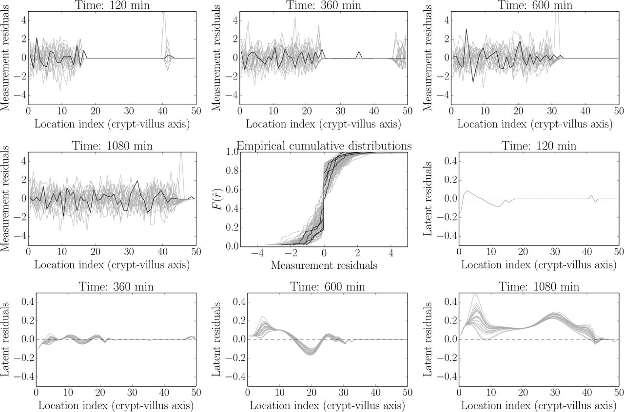
Model and data residual components. Panels 1-4, moving left-to-right and top-to-bottom, shows measurement error as determined by subtracting a smoothed spline from the observed data (dark line) and comparing this to the results obtained by subtracting the process model for fitted - 120, 360 and 600 mins - and unfitted/out-of-sample - 1080 min - times from the realised data (grey). These measurement error distributions are also visualised in terms of the corresponding cumulative distributions in the middle panel (panel 5, following as above. Black - actual data, grey - model simulations). Panels 6-9 show the differences between realisations of the underlying process model and the smoothed spline fitted to the data. As can be seen across panels, the measurement model appears approximately valid at all times, while the process model appears to have non-zero error for the 1080 min sample. This observation is discussed in the text.
Possible model improvement and robustness - higher-order spatial effects
As discussed in the process model section above, the presence of cellular structure in the epithelial tissue means that higher-order spatial effects may be present. Here we consider to what extent these may account for the minor misfit identified above.
To give an idea of the qualitative differences induced by including these higher-order terms, consider Fig (12) in which we compare to the (healthy) 1080 min (18 h) data in which we found some indication of a process model error. Note that while this model appears slightly better able to fit the qualitative features of the data, both models require similar modification of the parameter values to quantitatively improve the fit to our out-of-sample data (we have illustrated both for a case where parameter values are reduced by 20%). Thus the key (yet relatively small) difference between the model and out-of-sample data is likely due to an effect other than finite-cell sizes; for example it may be due to time-variation in parameter values due to circadian rhythms (we have assumed steady-state parameter values), label dilution or an unmodelled mixing phenomenon in the full two-dimensional case. We note however that these effects are small and appear to be important primilarly for predicting much further ahead in time than the fitted data and the steady-state parameter assumption is likely valid for reasonable time intervals. This means that the more easily interpretable original model may be sufficient for many purposes.
Discussion
Understanding the complicated dynamics of the intestinal epithelium requires an interdisciplinary approach involving experimental measurements, mathematical and computational modelling, and statistical quantification of uncertainties. While a diverse range of mathematical models have been constructed for epithelial cell and tissue dynamics (reviewed in Johnston et al. 2007; Carulli, Samuelson, and Schnell 2014; Kershaw et al. 2013; De Matteis, Graudenzi, and Antoniotti 2013; Fletcher, Murray, and Maini 2015), from compartment models to individual-based models to continuum models, we lack consistent and reproducible frameworks for comparing models representing conjectured biological mechanisms both to each other and to experimental data (for an overview, see our review Maclaren et al. 2015). These shortcomings may explain why questions such as the connection between proliferation and migration and its variation under experimental perturbations remain open, despite much investigation (Kaur and Potten 1986a; Kaur and Potten 1986b; Tsubouchi 1983; Loeffler et al. 1986; Loeffler et al. 1988; Meineke, Potten, and Loeffler 2001; Dunn, Näthke, and Osborne 2013).

Comparison of the modified process model which includes higher-order spatial terms (blue) to the original model (grey, dashed), both at lowered proliferation rates (decreased 20%), which is required for a better fit to the data. The original model at the original fitted proliferation rates is also shown (grey, solid). Although the model with higher-order spatial terms gives a better qualitative fit to the data for the same proliferation rates, it is clear that the dominant cause of misfit is better attributed to (time) varying proliferation rates (in the context of the present set of models).
The aim of the present work was to acknowledge and confront these difficulties explicitly, and to present some initial constructive steps in establishing such a framework. To do this we carried out new experiments (described more fully in a companion paper Parker et al. 2016) aimed at determining how proliferation rates, tissue growth and cellular migration rates are related in the intestinal epithelium under healthy, damaged (Ara-C treated) and recovering conditions. We performed BrdU/IdU cell-labelling experiments under these respective conditions. In considering how to best process these data and interpret them using mathematical models, we then developed a probabilistic, hierarchical (conditional) framework.
Our hierarchical framework provides a best-practice approach for systematically modelling and understanding the uncertainties that have, in our view, prevented past studies in this area from providing reliable mechanistic conclusions - uncertainties in experimental measurement and treatment, difficult-to-compare mathematical models of underlying mechanisms, and unknown or unobserved parameters. Our approach was influenced by recognising the benefits that the hierarchical Bayesian approach has demonstrated in applications across a number of different disciplines (e.g. in environmental and geophysical science as in Berliner 2003; Wikle 2003; ecological modelling as in Cressie et al. 2009; Ogle 2009; and in Bayesian statistical modelling and inverse problems more generally as in Berliner 1996; Tarantola 2005; Cressie and Wikle 2011; Wikle 2015; Gelman et al. 2013; Blei 2014). We also note that a hierarchical approach can have significant benefits outside the Bayesian framework (see for example the “extended likelihood” approach described in Pawitan 2001; Pawitan and Lee 2016; Lee, Nelder, and Pawitan 2006).
The hierarchical approach has advantages not only in terms of providing a framework for combining disparate sources of uncertainty, but also as a framework for facilitating modelling derivations and relating discrete and continuous models. Though the resulting measurement, process and parameter models can or have all been derived by other means, as far as we are aware this particular perspective has not been systematically utilised in the same manner as considered here - at the very least it appears uncommon within the mathematical/systems/computational biology communities. Furthermore, in the main text we noted the connections of our conditional, probabilistic approach for relating discrete and continuous models to similar procedures in the numerical analysis literature. This raises exciting connections to the developing field of probabilistic numerical methods and computing (Hennig, Osborne, and Girolami 2015).
We also note the connection between the choice of a measurement model as required here (and/or process model error, and following e.g. Berliner 1996; Berliner 2003; Wikle 2015; Cressie and Wikle 2011; Mosegaard and Tarantola 2002; Tarantola 2005), and the development of approximate sampling and parameter fitting procedures, which are particularly useful for analytically difficult models. A key concern of the latter is the appropriate choice of summary statistics for constructing a ‘synthetic likelihood’ (Wood 2010) or similarly-modified posterior target for Approximate Bayesian Computation (ABC) (Marin et al. 2012; Wilkinson 2013; Ratmann et al. 2009). This choice determines (implicitly or explicitly) in which ways a given model or set of models can be considered an ‘adequate’ representation of the data, which features are considered to be reproducible and what the associated ‘noise’ structure should be (Davies 2014 presents an alternative approach to characterising data features and model adequacy). These issues are crucial in deciding how to model the complexity of epithelial cell and tissue dynamics. An important next step, as described above, would be to bring more process model types and explicit measurement modelling into this framework and to evaluate and compare them under carefully modelled experimental conditions. Extensions incorporating other mechanical and/or cellular-level information (e.g. Dunn, Näthke, and Osborne 2013; Meineke, Potten, and Loeffler 2001) would provide a natural next step.
As a final methodogical point, by making our code and data available, as well as leveraging already-available open-source scientific Python software, we open up our work to other researchers to build on.
The main results establised using the above framework were
An adequate description of intestinal epithelial dynamics is achievable using a model based on purely proliferation-driven growth
This model is consistent with healthy, proliferation-inhibited (Ara-C-treated) and recovering conditions
The measurement and process model errors can be reasonably distinguished and checked separately
This checking indicates that much of the natural variability is directly attributable to the collection process and this process can be modelled in a simple manner
Possible model errors can also be identified and proposed explanations incorporated and tested within our framework, and thus the proper interpretation of experimental procedures is aided by using an explicit mathematical model and its predictive simulations
Including finite-cell-size effects gives a slightly better qualitative fit to experimental data, but the dominant sources of the long-time misfits are likely due to some other factor such as (relatively slowly) time-varying proliferation rates (e.g. due to circadian rhythms) or label dilution.
Acknowledgements
This work was funded by the BBSRC-UK, project numbers BB/K018256/1, BB/K017578/1, BB/K017144/1 and BB/J004529/1 and the EPSRC-UK, project number EP/I017909/1.
References


