

Abstract
Recent successes in genome-wide association studies (GWAS) make it possible to address important questions about the genetic architecture of complex traits, such as allele frequency and effect size. One lesser-known aspect of complex traits is the extent of allelic heterogeneity (AH) arising from multiple causal variants at a locus. We developed a computational method to infer the probability of AH and applied it to three GWAS and four expression quantitative trait loci (eQTL) datasets. We identified a total of 4152 loci with strong evidence of AH. The proportion of all loci with identified AH is 4-23% in eQTLs, 35% in GWAS of High-Density Lipoprotein (HDL), and 23% in schizophrenia. For eQTL, we observed a strong correlation between sample size and the proportion of loci with AH (R2=0.85, P = 2.2e-16), indicating that statistical power prevents identification of AH in other loci. Understanding the extent of AH may guide the development of new methods for fine mapping and association mapping of complex traits.
Allelic heterogeneity (AH), the presence of multiple variants at the same locus that influence a particular disease or trait, is the rule for Mendelian conditions. For example, approximately 100 independent mutations are known to exist at the cystic fibrosis locus1, and even more independent mutations are present at loci causing inherited haemoglobinopathies2. In contrast, the extent of AH at loci contributing to common, complex disease is almost unknown. Indeed, current GWAS studies assume the presence of a single causal variant at a locus and report the strongest signal. Most fine mapping methods that assume a single-variant model lack the power to detect the true causal variants3.
We developed and applied a new method to quantify the number of independent causal variants at a locus that are responsible for the observed association signals in GWAS. Our method is incorporated into the CAusal Variants Identification in Associated Regions (CAVIAR) software3. The method is based on the principle of jointly analyzing association signals (i.e., summary level Z-score) and LD structure in order to estimate the number of causal variants (see Methods). Our method computes the probability of having multiple independent causal variants by summing the probability of all possible sets of SNPs for being causal. We compared results from our method to results produced using the standard conditional method (CM)13, that tests for independent association of a variant after conditioning on its significantly associated neighbors.
To evaluate the performance of our method, we first simulated datasets with different number of causal variants (see Method section for about a detailed description of our simulated datasets). Our method detected AH with high accuracy (>80%) and outperformed the standard CM approach (see Supplementary Figures 1 and 2). Using our method, the rate of false positive (FP) was very low using different input parameters (Supplementary Figure 3), even when the true causal variant was not included or tagged (Supplementary Figure 4). We provide a more detailed description of our simulation and evaluation in the Method section.
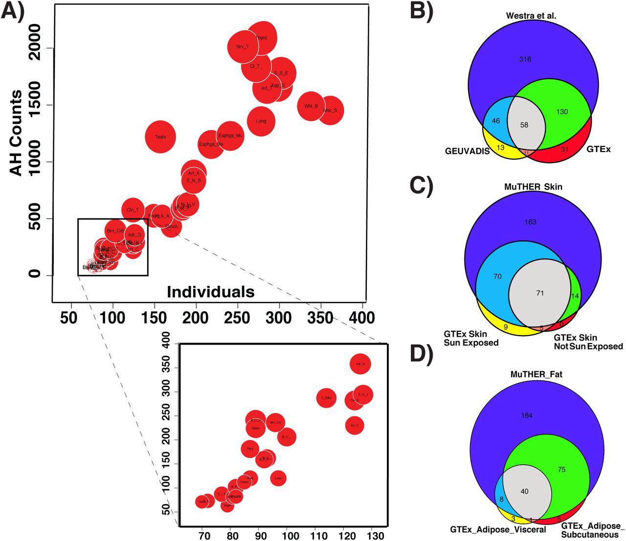
We used seven datasets to examine the extent of AH in complex traits. We first examined quantitative trait loci contributing to variation in transcript abundance (eQTL). In the Genotype Tissue Expression (GTEx) dataset4, we estimated the number of causal variants for genes that are known to have a significant cis eQTLs (eGene). We found that 4%-23% of the eGenes show evidence for AH (with probability > 80%) (Figure 1, Supplementary Table 1). The proportion of eGenes with AH for each tissue has a linear relationship with the sample size (R2=0.85, P = 2.2e-16), indicating that statistical power prevents the identification of AH at other loci. To check the reproducibility of these results, we compared the GTEx blood data with results from two other blood eQTL studies: GEUVADIS5 and Wester et al. (2013)6. We tested the overlap between genes with AH for skin and adipose tissues based on the GTEx and MuTHER dataset7. We only considered eGenes that are common between the studies. In all comparisons, we observed a high reproducibility for the detection of AH in blood (Figure 1B, P=7.9e-97), skin (Figure 1C, P=4.9e-63), and adipose (Figure 1D, P=1.1e-69) tissues.

Levels of allelic heterogeneity in eQTL studies. (A) Linear relationship between the amount of allelic heterogeneity and sample size. Each red circle indicates a different type of tissue from the GTEx dataset. The size of each red circle is proportional to the number of genes that harbor a significant eQTL (eGenes). (B-D) Significant overlap between allelic heterogeneity estimations for different eQTL datasets, shown for (B) blood (P=7.9e-97), (C) skin (P=4.9e-63), and (D) adipose (P=1.1e-69).
To measure the level of AH in a human quantitative trait, we applied our method to a GWAS of High-Density Lipoprotein (HDL)8. Out of 37 loci, 13 (35%) showed evidence for AH with probability > 80% (see Supplementary Table 2). We also studied the results of GWASs focused on two psychiatric diseases, major depression9 and schizophrenia10. For depression, we found evidence for AH at one of two loci. For schizophrenia (SCZ), we identified 25 loci out of 108 (23%) with high probability of AH (see Supplementary Table 3). One example of AH in SCZ is the locus on chromosome 18 that includes the TCF4 gene (Figure 2a). The locus contains multiple associated SNPs that are distributed in different LD blocks (Figure 2b). According to our analysis, there are three or more causal variants in this locus with high probability (Figure 2c) (for similar results in other loci, see Supplementary Figures 6-41 for HDL and Supplementary Figures 42-169 for SCZ).

Allelic heterogeneity in the TCF4 locus associated with schizophrenia. (A) Manhattan plot obtained from Ricopili (http://data.broadinstitute.org/mpg/ricopili/) consists of all the variants in a 1Mbp window centered on the most significant SNP in the locus (rs9636107). This plot indicates multiple significant variants that are not in tight LD with the peak variant. (B) LD plot of the 50 most significant SNPs showing several distinct LD blocks. (C) Histogram of the estimated number of causal variants.
We have shown that allelic heterogeneity is widespread and more common than previously estimated in complex traits. Since our method is influenced by statistical power and by uncertainty induced by LD, the proportions of loci with AH detected in this study are just a lower bound on the true amount of AH. Thus, our study suggest that many, if not most, loci are affected by allelic heterogeneity. Our results highlight the importance of accounting for the presence of multiple causal variants when characterizing the mechanism of genetic association in complex traits.
Online Methods
Overview of Methods
The input to our method is the LD structure of the locus and the marginal statistics for each variant in the locus. The LD between each pair of variants is computed from genotyped data or is approximated from HapMap11 or 1000G12 data. We use the fact that the joint distribution of the marginal statistics follows a multivariate normal distribution (MVN) to compute the posterior probability of each set of variants being causal, as described below. Then, we compute the probability of having i independent causal variants in a locus by summing the probability of all possible sets of size i (sets that have i causal variants). We consider a locus to be AH when the probability of having more than one independent causal variant is more than 80%.
We would like to emphasize that using only summary statistics is not sufficient to detect AH in some cases. For example, it is impossible to detect the true number of causal variants using only the summary statistics and LD for a locus that contains several causal variants with perfect pair-wise LD. Therefore, our estimates are just a lower bound on the amount of AH for a given complex trait.
The Generative Model
We utilize the fact that the vector of observed marginal statistics (e.g., the z-score) follows a multivariate normal (MVN) distribution3. Let S = [s1, s2, s3, …sm]T indicate the observed marginal statistics for a locus with m variants. In addition, Σ is a (m × m) matrix that encodes the genotype pair-wise correlations. We denote the LD structure with Σ. The joint distribution of observed marginal statistics is as follows:
 , where Λ =[λ1, λ2, … λm]T is a vector of effect sizes and λi is the effect size of the ith variant. In this setting, λi is set to zero if the i-th variant is non-causal, and it is set to non-zero if the variant is causal. Let C=[c1, c2, ..cm]T denote the vector of causal status. Causal status for one variant can have two possible values: zero and one. Causal status of zero indicates the variant is non-causal, and causal status of one indicates the variant is causal. Similar to the method of our previous study3, we define the joint distribution of effect sizes following a MVN distribution:
 , where Σc is a (m × m) diagonal matrix. Diagonal elements of matrix Σc are set to zero for variants that are non-causal. Thus, using the conjugate prior, we have:

We provide a more detailed description of the model in Supplementary Text.
Computing the Number of Independent Causal Variants
We compute the probability of having i independent causal variants in a locus as the summation of all possible causal configurations where exactly i variants are causal. Let Nc indicate the number causal variants in a locus. We have:
 , where P(C) is the prior on the causal configuration C, C is the set of all possible causal configurations – including the configuration all the variants are not causal – and |C| indicates the number of causal variants in the causal configuration C. The numerator in the above equation considers all possible causal configurations that have i causal variants. The denominator is a normalization factor to ensure that the probability definition holds. We define the prior probability as
  . In our experiment, we set γ to 0.001 (see Supplementary Text).
Although computing the probability of each causal configuration requires O(m3) operations, we utilize the matrix structure of the marginal statistics to reduce this computation (see Supplementary Text). Our reduction is in a factor of m/k, where k is the number of causal variants for each causal configuration. Thus, in our method, we require O(m2k) operations to compute the likelihood of each causal configuration.
Conditional Method (CM)
A standard method to detect allelic heterogeneity (AH) is the conditional method (CM). In CM, we identify the SNP with most significant association statistics. Then, conditioning on that SNP, we re-compute the marginal statistics of all the remaining variants in the locus. We consider a locus to have AH when the re-computed marginal statistics for at least one of the variants is more significant than a predefined threshold. Similarly, we consider a locus to not have AH when the re-computed marginal statistics of all variants fall below the predefined threshold. The predefined threshold is referred to as the stopping threshold for CM. This standard method can be applied to either summary statistics or individual level data13. GCTA-COJO13 performs conditional analysis while utilizing the summary statistics.
When applying CM to individual level data, we re-compute the marginal statistics by performing linear regression where we add the set of variants that are selected as covariates.
We utilize the LD between the variants, which we obtain from a reference dataset, when applying CM to summary statistics data. In this case, we re-compute the marginal statistics for the ith variant as follows:
 when we have selected the jth variant as causal. Let zi indicate the marginal statistics for the ith variant and rij the genotype correlations between the ith and jth variants.
Datasets
Genotype-Tissue Expression (GTEx):
We obtained the summary statistics for GTEx4 eQTL dataset (Release v6, dbGaP Accession phs000424.v6.p1) at http://www.gtexportal.org. We estimated the LD structure using the available genotypes in the GTEx dataset. We considered 44 tissues and applied our method to all eGenes, genes that have at least one significant eQTL, in order to detect loci that harbor allelic heterogeneity..
Genetic European Variation in Disease (GEUVADIS):
We obtained the summary statistics of blood eQTL for 373 European individuals from the GEUVADIS5 website (ftp://ftp.ebi.ac.uk/pub/databases/microarray/data/experiment/GEUV/E-GEUV-1/analysis_results/). We approximated LD structure from the 1000G CEU population. We applied our method to the 2954 eGenes in GEUVADIS to detect AH loci.
Multiple Tissue Human Expression Resource (MuTHER):
We obtained the summary statistics from MuTHER6 website (http://www.muther.ac.uk/Data.html). We utilized the skin and fat (adipose) tissues. We then approximated LD from the 1000G CEU population. We obtained 1433 eGenes for skin and 2769 eGenes for adipose.
High-Density Lipoprotein Cholesterol (HDL-C):
We used the High-Density Lipoprotein Cholesterol (HDL-C) trait8. We only considered the GWAS hits, which are reported in a previous study8. We applied ImpG-Summary14 to impute the summary statistics with 1000G as the reference panel. We identified 37 loci that have at least one causal variant. Following common protocol in fine-mapping methods, we assumed at least one causal variant.. Then, we applied our method to each locus.
Psychiatric diseases:
We analyzed the recent GWAS on major depression9 and schizophrenia10. The major depression study has 2 and the schizophrenia study has 108 loci identified to contain at least one significant variant. We utilized the summary statistics provided by each study and approximated the LD using the 1000G CEU population.
Data simulation
We first simulated genotypes using HAPGEN215, where we utilized the 1000G CEU population as initial reference panels. Then, we simulated phenotypes using the Fisher’s polygenic model, where the effects of causal variants are obtained from the normal distribution with a mean of zero. We let Y indicate the phenotypes and X indicate the normalized genotypes. In addition, β is the vector of effect sizes where βi is the effect of the i-th variant. Thus, we have:
 , where e models the environment and measurement noise. Under the Fisher’s polygenic model, the effect size of the causal variants is obtained from
  , where Nc is the number of causal variants and σg is the genetic variation. In addition, the effect size for variants that are non-causal is zero. We set the effect size in order to obtain the desired statistical power. We implanted one, two, or three causal variants in our simulated datasets.
We use false positive (FP) and true positive (TP) as metrics to compare different methods. FP indicates the fraction of loci that harbor one causal variant and are incorrectly detected as loci that harbor AH. TP indicates the fraction of loci that harbor AH and are correctly detected.
Code availability
Our method is incorporated into CAVIAR software that is available at http://genetics.cs.ucla.edu/caviar
Acknowledgments
FH, JWJJ, and EE are supported by National Science Foundation grants 0513612, 0731455, 0729049, 0916676, 1065276, 1302448, 1320589 and 1331176, and National Institutes of Health grants K25-HL080079, U01-DA024417, P01-HL30568, P01- HL28481, R01-GM083198, R01-ES021801, R01-MH101782 and R01-ES022282. EE is supported in part by the NIH BD2K award, U54EB020403. AVS is supported by a contract (HHSN268201000029C) to the Laboratory, Data Analysis, and Coordinating Center (LDACC) at The Broad Institute, Inc. SS was supported in part by NIH grant R00-GM 111744-03. GK is supported by the Biomedical Big Data Training Program (NIH-NCI T32CA201160). We acknowledge the support of the NINDS Informatics Center for Neurogenetics and Neurogenomics (P30 NS062691).


