

Abstract
FST and kinship are key parameters often estimated in modern population genetics studies. Kinship matrices have also become a fundamental quantity used in genome-wide association studies and heritability estimation. The most frequently used estimators of FST and kinship are method of moments estimators whose accuracies depend strongly on the existence of simple underlying forms of structure, such as the island model of non-overlapping, independently evolving subpopulations. However, modern data sets have revealed that these simple models of structure do not likely hold in many populations, including humans. In this work, we provide new results on the behavior of these estimators in the presence of arbitrarily complex population structures. After establishing a framework for assessing bias and consistency of genome-wide estimators, we calculate the accuracy of FST and kinship estimators under arbitrary population structures, characterizing biases and estimation challenges unobserved under their originally assumed models of structure. We illustrate our results using simulated genotypes from an admixture model, constructing a one-dimensional geographic scenario that departs nontrivially from the island model. Using 1000 Genomes Project data, we verify that population-level pairwise FST estimates underestimate differentiation measured by an individual-level pairwise FST estimator introduced here. We show that the calculated biases are due to unknown quantities that cannot be estimated under the established frameworks, highlighting the need for innovative estimation approaches in complex populations. We provide initial results that point towards a future estimation framework for generalized FST and kinship.
1 Introduction
In population genetics studies, one is often interested in characterizing structure, genetic differentiation, and relatedness among individuals. Two quantities often considered in this context are FST and kinship. FST is a parameter that measures structure in a subdivided population, satisfying FST = 0 for an unstructured population and FST = 1 if every SNP has fixated in every subpopulation. More specifically, FST is the probability that alleles drawn randomly from a subpopulation are “identical by descent” (IBD) relative to an ancestral population [1, 2]. The kinship coefficient is a measure of relatedness between individuals defined in terms of IBD probabilities, and it is closely related to FST [1].
The most frequently used FST estimators are derived and justified under the “island model” assumption, in which subpopulations are non-overlapping and have evolved independently from a common ancestral population. The Weir-Cockerham (WC) FST estimator assumes islands of differing sample sizes and equal FST per island [3]. The “Hudson” FST estimator assumes two islands with different FST values [4]. These FST estimators are ratio estimators derived using the method of moments to have unbiased numerators and denominators, which gives approximately unbiased ratio estimates [3–5], and they are important contributions used widely in the field.
Kinship coefficients are now commonly calculated in population genetics studies to capture structure and relatedness. They are utilized in principal components analyses and linear-mixed effects models to correct for structure in Genome-Wide Association Studies (GWAS) and to estimate genome-wide heritability [6–15]. The most commonly used kinship estimator for genotype data [9, 10, 13–18] is also a method of moments estimator whose operating characteristics are largely unknown in the presence of structure. As we show here, the required assumption for this popular estimator to be accurate is that the average kinship be zero, which implies that the population must be unstructured.
Recent genome-wide studies have revealed that humans and other natural populations are structured in a complex manner that violate the assumptions of the above estimators. This has been observed in several large human studies, such as the Human Genome Diversity Project [19], the 1000 Genomes Project [20], and other contemporary [21, 22] and archaic populations [23, 24]. Therefore, there is a need for innovative approaches designed for complex population structures. To this end, we reveal the operating characteristics of these frequently used FST and kinship estimators in the presence of arbitrary forms of structure with the goal of identifying new estimation strategies for FST and kinship.
We generalized the definition of FST for arbitrary population structures in the first paper in this series [25]. Additionally, we derived connections between FST and three models: arbitrary kinship coefficients [1, 26], individual-specific allele frequencies [27, 28], and admixture models [29–31]. Here, we study existing FST and kinship method of moments estimators in models that allow for arbitrary population structures (see Fig. 1 for an overview of the results). First, we obtain new strong convergence results for a family of ratio estimators that includes FST and kinship estimators. Next, we calculate the convergence values of these estimators under arbitrary population structures, where we find biases that are not present under their original assumptions about structure. We characterize the limit of the standard kinship estimator for the first time, identifying complex biases or distortions that have not been described before. We construct an admixture model, which represents a form of structure distinct from the island model, to illustrate our theoretical findings through simulation. We analyze 1000 Genomes Project populations to illustrate their non-island nature, and measure differentiation that is missed by the Hudson FST estimator. We identify a new direction for estimating FST and kinship in a nearly unbiased fashion, which is the topic of our next paper in this series [32].

Our analysis is based on two parallel models: the coancestry model for individual-specific allele frequencies (πij), and the kinship model for genotypes (xij). The kinship  and coancestry
  parameters are closely related as shown. We use these models to study the accuracy of FST and kinship method of moment estimators under arbitrary population structures. The bias resulting from the misapplication of the FST island model estimator
  to arbitrary structures is calculated under the coancestry model, while the bias in the standard kinship model estimator
  and its resulting plug-in FST estimator
  is calculated under the kinship model. We present a new kinship estimator
  with a uniform bias, which will be used to obtain more accurate kinship estimates in the next paper in the series (starting from
  ). Lastly, we present a new pairwise FST estimator for two individuals
  that is unbiased for the true pairwise FST that we introduced in our previous work. Note that estimation of FST and Fjk from genotypes requires individuals to be locally outbred and locally unrelated.
2 Models and definitions
Here we summarize new arbitrary population structure models, definitions, and results presented in detail in the first paper in this series [25] (Fig. 1). We assume a complete matrix of m SNPs and n individuals. We concentrate on biallelic genotypes xij for SNP i and individual j, encoded as the number of reference alleles: xij = 2 is homozygous for the reference allele, xij = 0 is homozygous for the alternative allele, and xij = 1 is heterozygous. We assume the existence of a panmictic ancestral population T characterized by ancestral reference allele frequencies  ∈ (0, 1) for every SNP i.
2.1 The kinship model and the generalized FST
Under the kinship model, individuals receive their alleles as determined by their inbreeding and kinship coefficients. The inbreeding coefficient  of j is the probability that two alleles at a random SNP of individual j are IBD [33]. Similarly, the kinship coefficient
  of j and k is the probability that two alleles chosen at random from each individual and at a random SNP are IBD [1]. The ancestral population T determines what is IBD: only relationships since T count toward IBD. The first two moments of the genotypes are

 where self-kinship is
  [1, 2, 26, 33]. Lastly, if S is a panmictic population that evolved from T, then
  is the value of
  shared by all individuals j in S relative to T, and equals Wright’s FST for this subdivided population [2].
The generalized FST definition that we proposed [25] requires the notion of local populations, needed to mirror at the individual level Wright’s distinction between structural inbreeding due to the population structure from local inbreeding [2]. The local population Lj of individual j is the most recent ancestral population of j [25]. Similarly, the jointly local population Ljk of a pair of individuals j and k is the most recent ancestral population shared by j and k, which is ancestral to both Lj and Lk [25]. For T ancestral to Lj or Ljk, as needed, we have three parameter pairs: “total”  , “local”
  , and “structural”
  kinship and inbreeding coefficients, related by [25]
 A locally outbred individual has
  and therefore
  . Similarly, a pair of locally unrelated individuals have
  and therefore
  . The generalized FST is given by
 where wj > 0,
  are weights chosen to capture the sampling procedure of individuals [25]. The individual-level pairwise FST is the special case of Eq. (4) for n = 2 individuals, given by
 where the second equality holds for any T ancestral to Ljk [25].
2.2 The coancestry model for individual-specific allele frequencies
Previous FST estimators are often in terms of population allele frequencies [2–5]. Our earlier proposed coancestry model [25] extends previous models [5, 34] of population allele frequencies to individuals. The individual-specific allele frequency (IAF) is denoted πij ∈ [0, 1] for SNP i and individual j [27, 28]. In our model, IAFs are random variables drawn from T according to the population structure, with covariances between individuals j and k parametrized by the individual-specific coancestry coefficients  . We assume that the IAF moments and genotypes are drawn as


 We derived the following correspondence between coancestry and kinship coefficients by marginalizing πij from this model and comparing to Eqs. (1) and (2) [25]:
 For this reason, and the similarities between Eqs. (1) and (2) and Eqs. (6) and (7), estimators based on genotypes can be readily restated in terms of IAFs, and viceversa. Due to Eq. (8), individuals in the coancestry model are locally outbred and unrelated, a key difference from the more general kinship model, so
  and
and  for j ≠ k also hold. Therefore, FST in this model equals

3 Assessing the accuracy of genome-wide estimators
Many FST and kinship coefficient method of moments estimators are “ratio estimators”, a class that tends to be biased and have no closed form expectation [35]. In the literature, the expectation of a ratio is frequently approximated with a ratio of expectations [3–5]. Specifically, estimators are often called “unbiased” if the ratio of expectations is unbiased, even though the ration estimator itself may be biased. Here we characterize the behavior of two ratio estimator families calculated from genome-wide data, detailing conditions where this previous approximation is justified and providing additional criteria to assess the accuracy of such estimators.
The general problem involves random variables ai and bi calculated from genotypes at each SNP i, such that E[ai] = Aci and E[bi] = Bci and the goal is to estimate  . A and B are constants shared across SNPs (given by FST or
  ), while ci depends on the ancestral allele frequency
  and varies per SNP. The problem is that the single SNP estimator
  is biased, since
  [35]. Below we study two estimator families that combine SNPs to better estimate
  .
.
The solution we recommend is the “ratio-of-means” estimator  , where
  and
and  , which is common for FST estimators [3–5]. Note that
  and
and  , where
  . We will assume bounded terms (|ai|, |bi| ≤ C for some finite C), a convergent
  , and Bc ≠ 0, which are satisfied by common estimators. Given independent SNPs, we prove almost sure convergence to the desired quantity (Appendix A.1),
 a strong result that implies
  , justifying previous work [3–5]. Moreover, the error between these expectations scales with
  (Appendix A.2), just as for standard ratio estimators [35]. Although real SNPs are not independent due to genetic linkage, this estimator will perform well if the effective number of independent SNPs is large.
Another approach is the “mean-of-ratios” estimator  , used often to estimate kinship coefficients [9, 10, 13–18] and FST [20]. If each
  is biased, their average across SNPs will also be biased, even as m → ∞. However, if
  for all SNPs i = 1, …, m as the number of individuals n → ∞, and Var
  is bounded, then
 Therefore, mean-of-ratios estimators must satisfy more restrictive conditions than ratio-of-means estimators, as well as both large n and m, to estimate
  well.
well.
4 FST estimation based on the island model
4.1 The island model FST estimator for infinite population sample sizes
Here we study the Weir-Cockerham (WC) [3] and “Hudson” [4] FST estimators, which assume the island model. These method of moment estimators have small sample size corrections that remarkably make them consistent as the number of independent SNPs m goes to infinity for finite numbers of individuals. However, these small sample corrections also make the estimators more notationally cumbersome than needed here. In order to illustrate clearly how these estimators behave, both under the island model and arbitrary structure, here we construct simplified versions that assume infinite sample sizes per population. This simplification corresponds to eliminating statistical sampling, leaving only genetic sampling to analyze [36]. Note that our simplified estimator nevertheless illustrates the general behavior of the WC and Hudson estimators under arbitrary structure, and the results are equivalent to those we would obtain under finite sample sizes of indivduals.
The Hudson FST estimator compares two populations [4]; we present a generalized Hudson estimator for K populations in Appendix B. Let us assume that population sample sizes are infinite, so allele frequencies are known. Let j index populations rather than individuals, n be the number of populations, and πij be the allele frequency in population j at SNP i. In this special case, both WC and Hudson simplify to the following island model FST estimator:


 The goal is to estimate FST of Eq. (10) with uniform weights
  , under our coancestry model defined in Eqs. (6) – (8).
4.2 FST estimation under the island model
Under the island model,  for j ≠ k, the estimator of Eq. (14) can be derived directly using the method of moments (Appendix C.1). Given the IAF moment Eqs. (6) and (7), the expectations of the two recurrent terms of Eq. (14) are
 Eliminating
  and solving for FST in this system of equations recovers the estimator of Eq. (14).
Before applying the convergence result of Eq. (11), we test that its assumptions are met. The SNP i terms are  and
and  , which satisfy E[ai] = Aci and E[bi] = Bci with A = FST, B = 1, and
  . Further,
  over the
  distribution across SNPs. Lastly, since
  hold, then
  and
and  , and since n ≥ 2, C = 1 bounds both |ai| and |bi|. Therefore, for independent SNPs,

4.3 FST estimation under arbitrary coancestry
Now we consider applying the island FST estimator to non-island settings. The key difference is that  for every (j, k) will be assumed in our coancestry model of Eqs. (6) and (7). In this general setting, (j, k) may index either populations or individuals. The two terms of
  now satisfy
 where
where  is the mean coancestry with uniform weights. There are two equations but three unknowns: FST,
  , and
, and  . Island models satisfy
  , which allows for the consistent estimation of FST. Therefore, the new unknown
  precludes consistent FST estimation without additional assumptions.
The island model FST estimator converges more generally to
 where it should be noted that
 is the average of all between-individual coancestry coefficients, a term that appears in a related result for populations [5]. Therefore, under arbitrary structure the island model estimator’s bias is due to the coancestry between individuals (or islands in the traditional, non-overlapping subpopulation setting).
Since  (Appendix D), this estimator has a downward bias in non-island settings: it is asymptotically unbiased
  only when
  , while bias is maximal when
  , where
  . For example, if
  for most pairs of individuals, then
  as well, and
  . Therefore, the magnitude of the bias of
  is unknown if
  is unknown, and small
  may arise even if FST is very large.
4.4 Consistent estimator of the individual-level pairwise FST
The individual-level pairwise FST, equal to FST for n = 2 and denoted by Fjk, is always an island model since T = Ljk must the most recent ancestral population shared by (j, k) and satisfies  [25]. Hence, Fjk can be estimated consistently using
  of Eq. (14) with n = 2, which simplifies to
 where the limit is stated for general T ≠ Ljk and matches Fjk under the coancestry model [25].
To obtain an estimator of Fjk that uses genotypes, we replace πij by  in Eq. (16) and convert kinship to inbreeding coefficients using
  , resulting in
 which converges to Fjk in Eq. (5) if j and k are locally outbred and locally unrelated
  . For general values of
  , and
, and  ,
,
 which is obtained by substituting Eq. (3) into Eq. (17) and rearranging. Since
  is the only negative term in Eq. (18), local kinship can result in negative
  estimated from genotypes.
To compare our individual-level estimates to Hudson estimates between the two populations Su and Sv that are not necessarily panmictic, consider the following average  across populations and its limit assuming locally outbred and locally unrelated individuals:
 If Su and Sv are panmictic populations, then Lj = Su, Lk = Sv, and Ljk = Luv, so every pair and their average
  match the limit of the Hudson estimator. In Section 7, we show empirically that
  tends to be larger than the corresponding Hudson estimate when Su and Sv are structured.
4.5 Coancestry estimation as a method of moments
Since the generalized FST is given by coancestry coefficients  in Eq. (10), a new FST estimator could be derived from estimates of
  . Here we attempt to define a method of moments estimator for
  , and find an underdetermined estimation problem, just as for FST.
Given IAFs and Eqs. (6) and (7), the first and second moments that average across SNPs are

 where
where  , and
, and  is as before.
Suppose first that only  are of interest. There are n estimators given by Eq. (21) with j = k, each corresponding to an unknown
  . However, all these estimators share two nuisance parameters:
  and
and  . While
  can be estimated from Eq. (20), there are no more equations left to estimate
  , so this system is underdetermined. The estimation problem remains underdetermined if all
  estimators of Eq. (21) are considered rather than only the j = k cases. Therefore, we cannot estimate coancestry coefficients consistently using only the first two moments and without additional assumptions.
5 Characterizing a kinship estimator and its relationship to FST
Estimation of kinship coefficients is an important problem, particularly for GWAS approaches that control for population structure [6–18, 37, 38]. Additionally, kinship coefficients are closely related to the generalized FST of Eq. (4) and the biases of  in Eq. (15) (since coancestry and kinship coefficients are related by Eq. (3)). In this section, we focus on a standard kinship method of moments estimator and calculate its limit for the first time (Fig. 1). We study estimators that use genotypes or IAFs, and construct FST estimators from their kinship estimates. We find biases comparable to those of
  , and define unbiased FST estimators that require knowing the mean kinship or coancestry, or its proportion relative to FST. Lastly, we present a new kinship method of moments estimator with a uniform bias, which facilitates the estimation of the unknown mean kinship parameter needed to unbias kinship and FST estimates (Fig. 1).
5.1 Characterization of the standard kinship estimator
Here we analyze a standard kinship estimator that is in frequent use [9, 10, 13–18]. We generalize this estimator to use weights in estimating the ancestral allele frequencies, and we write it as a ratio-of-means estimator due to the favorable theoretical properties of this format as detailed in Section 3:

 The estimator in Eq. (23) resembles the sample genotype covariance, but centers by SNP i rather than by individuals j and k, and normalizes by estimates of
  . We also derive the estimator of Eq. (23) directly using the method of moments (Appendix C.2). The weights in Eq. (22) must satisfy wj > 0 and
  , so
, so  and
and  hold.
hold.
Assuming the moments of Eqs. (1) and (2), we find that Eq. (23) converges to
 where
where  and
and  . (See Appendix E for moments involving xij and
  that lead to Eq. (24).) Therefore, the bias of
  varies per j and k. Analogous distortions have been observed for sample covariances of genotypes [39]. Similarly, inbreeding coefficient estimates derived from Eq. (23) converge to
 The limits of the ratio-of-means versions of two more
  estimators [14] are, if
  uses Eq. (22),

The estimators of Eqs. (23) and (26) are unbiased when  is replaced by
  [10, 14], and are consistent when
  is consistent [27]. Surprisingly,
  of Eq. (22) is not consistent (it does not converge almost surely) for arbitrary population structures, which is at the root of the bias of Eq. (24). In particular, although
  is unbiased, its variance (see Appendix E),
 may be asymptotically non-zero as n → ∞, since
  ∈ (0, 1) is fixed and
  may take on any value in [0, 1] for arbitrary population structures. Further,
  as n → ∞ if and only if
  for almost all pairs of individuals (j, k). These observations hold for any weights such that wj > 0,
  . An important consequence is that the plug-in estimate of
  is biased (Appendix E),
 which is present in all estimators we have studied.
5.2 Estimation of coancestry coefficients from IAFs
Here we form a coancestry coefficient estimator analogous to Eq. (23) but using IAFs. Assuming the moments of Eqs. (6) and (7), this estimator and its limit are

 where
where  and
and  are analogous to
  and
and  . Eq. (28) generalizes Eq. (12) for arbitrary weights. Thus, use of IAFs does not ameliorate the estimation problems we have identified for genotypes. Like Eq. (27),
  of Eq. (28) is not consistent because Var
  , which causes the bias observed in Eq. (29).
5.3 Plug-in Fst estimator from inbreeding or coancestry estimates
Since the generalized FST is defined as a mean inbreeding coefficient in Eq. (4), or equivalently a mean self-coancestry coefficient in Eq. (10), here we study FST estimators constructed as either  or
or  . Although the previous
  and
and  are biased, we nevertheless plug them into our definition of FST so that we may study how bias manifests. Note that we do not recommend utilizing these FST estimators in practice, but we find these results informative for identifying how to proceed in deriving new estimators.
Remarkably, the three  estimators of Eqs. (25) and (26) give exactly the same plug-in
  if the weights in FST and
  of Eq. (22) match, namely
 where the limit assumes locally outbred individuals so
  holds. The analogous FST estimator for IAFs and its limit are
 The estimators of Eqs. (30) and (31) for individuals and their limits resemble those of classical FST estimators for populations of the form
  [5, 34].
  of Eq. (31) for uniform weight is also GST for a biallelic locus [40] if we treat individuals j as populations and combine SNPs as a ratio-of-means estimator. Compared to
  of Eq. (14),
  of Eq. (31) admits arbitrary weights and, by forgoing bias correction under the island model, is a simpler target of study.
Like  of Eq. (14),
  of Eqs. (30) and (31) are downwardly biased since
  .
.  of Eq. (31) may converge arbitrarily close to zero since
  can be arbitrarily close to FST (Appendix D). Moreover, although
  for large n (due to Eq. (9)), in extreme cases
  can exceed FST under the coancestry model (where
  holds) and also under extreme local kinship, where
  of Eq. (30) converges to a negative value.
5.4 Adjusted consistent FST estimators and the “bias coefficient”
Here we explore two adjustments to  from IAFs of Eq. (31) that rely on having minimial additional information needed to correct its bias. If
  is known, the bias in Eq. (31) can be reversed, yielding the consistent estimator
 Consistent estimates are also possible if a scaled version of
  is known, namely
 which we call the “bias coefficient” and has interesting properties. This coefficient measures the strength of the covariances relative to the variances, and satisfies 0 ≤ s ≤ 1 (Appendix D). The limit of Eq. (31) in terms of s is
 Treating the limit as equality and solving for FST yields the following consistent estimator:

 Note that
  and
and  from Eqs. (13) and (14) are the special case of Eqs. (35) and (36) for uniform weights and
  ; hence,
  generalizes
  .
.
Lastly, using either Eq. (31) or Eq. (34), the relative error of  converges to
 which is approximated by s if FST ≪ 1, hence the name “bias coefficient”.
5.5 A new direction for FST and kinship estimation
Here, we outline a new estimation framework for kinship coefficients that has properties favorable for obtaining nearly unbiased estimates. These new kinship estimates can then also be utilized for FST estimation. We summarize our ideas here and then fully develop the estimation framework and study its operating characteristics in the next paper in this series [32].
Applying the method of moments to Eqs. (1) and (2), we derive the following estimator,
 which compares favorably to the standard estimator of Eq. (24) by having a uniform bias in the limit, controlled by the sole parameter
  . If
. If  were known, Eq. (38) could be adjusted to yield unbiased kinship estimates:
 Remarkably, Eq. (38) itself can be used to estimate
  : assuming
  and a large number of SNPs m, then
 from which
  can be solved. However, additional steps can be taken to provide a more stable estimate than that based on
  [32]. Our improved kinship estimator will result in a plug-in FST estimator with increased accuracy.
The analogous coancestry estimator using IAF is
 Lastly, note that the inbreeding coefficient estimator derived from Eq. (38) using
  equals
  of Eq. (26), so the resulting plug-in FST estimator equals that of Eq. (30). Therefore, Eq. (38) by itself does not directly yield a new FST estimator.
6 An admixture simulation illustrates challenges in FST and kinship estimation
6.1 Overview of simulations
We simulate genotypes from two models to illustrate our results when the true population structure parameters are known. One is an island model, the other an admixture model differing from the island model by its pervasive covariance, and designed to induce large biases in existing FST estimators (Fig. 2). Both simulations have n = 1000 individuals, m = 300, 000 SNP loci, and K = 10 islands or intermediate populations. These simulations have FST = 0.1, comparable to estimates between human populations [4].

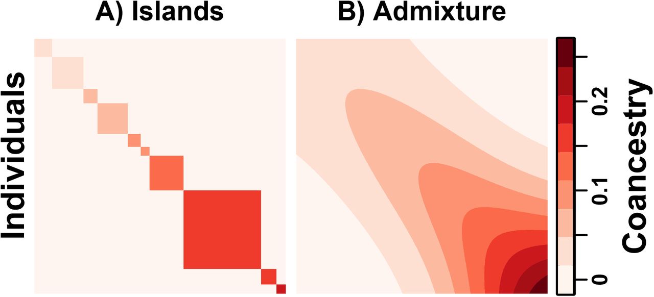
Both simulations have n = 1000 individuals along both axes, K =10 populations (islands or intermediate), and FST = 0.1. Color corresponds to  between individuals j and k. A) The island model has
  between islands, and varying
  per island, resulting in a block-diagonal covariance matrix. B) Our admixture scenario models a 1D geography with extensive admixture and intermediate population differentiation that increases with coordinate. Individuals are ordered by their coordinate in the 1D geography.
Our island model satisfies the Hudson estimator assumptions: populations are independent, and each population Su has a different FST value of  (Fig. 2A). Ancestral allele frequencies
  are drawn uniformly in [0.01, 0.5]. Allele frequencies
  for Su and SNP i are drawn independently from the Balding-Nichols (BN) distribution [41] with parameters
  and
and  . Every individual j in island Su draws alleles randomly with probability
  . Podpulation sample sizes were drawn randomly (Appendix F).
Our admixture model is a “BN-PSD” model [9, 17, 25, 27, 42, 43], which we analyzed in our previous paper in this series [25]. The intermediate populations are islands that draw  from the BN model, then each individual j constructs its allele frequencies as
  , which is a weighted average of
  with the admixture proportions qju of j and u as weights (which satisfy
  , as in the Pritchard-Stephens-Donnelly [PSD] admixture model [29–31]). We constructed qju that model admixture resulting from spread by random walk of the intermediate populations along a one-dimensional geography, as follows. Intermediate populations Su are placed on a line with differentiation
  that grows with coordinate (Fig. 3A). Upon differentiation, individuals in each Su spread with random walks, a process modeled by Normal densities (Fig. 3B). Admixed individuals derive their ancestry proportional to these Normal densities, resulting in a genetic structure governed by geography (Fig. 3C, Fig. 2B) and departing strongly from the island model (Fig. 3D). The amount of spread was chosen to give s = 0.5, which by Eq. (37) results in a large bias for
  (in contrast, the island simulation has s = 0.1). See Appendix F for additional details regarding these simulations.
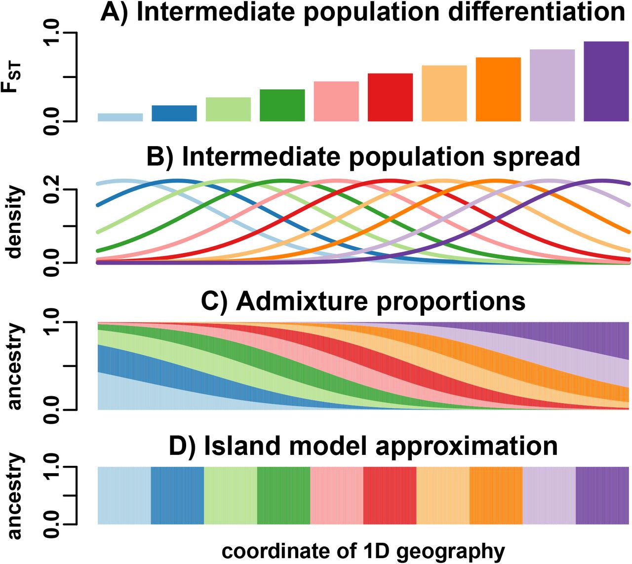
We model a 1D geography population that departs strongly from the island model. A) K = 10 intermediate populations, placed equidistant on a line, evolve independently with FST increasing with x-coordinate. B) Once differentiated, these intermediate populations spread by random walks modeled by Normal densities. C) n = 1000 individuals, sampled in equal intervals in the same range, are admixed proportionally to the previous Normal densities. D) To apply the WC and Hudson FST estimators, individuals are assigned to populations (“islands”) by their majority ancestry.
6.2 Weir-Cockerham and Hudson FST estimators misapplied to an admixed population
Our admixture simulation illustrates the large biases that can arise if the WC and Hudson FST estimators are misapplied to non-island populations to estimate the generalized FST. First, we test these estimators in our island model. This simulation satisfies the assumptions of the Hudson estimator (which we generalized for K population islands in Appendix B), so it is consistent (Fig. 4A). The WC estimator assumes that  for all u, which does not hold; nevertheless, WC has a small bias (Fig. 4A). For comparison, we added the “plug-in” FST estimator of Eq. (30) (weights from Appendix F), which is derived from the kinship estimator of Eq. (23) and does not have island model corrections. Since the number of islands K is large, the plug-in estimator has a small relative bias of about
  ; greater bias is expected for smaller K.
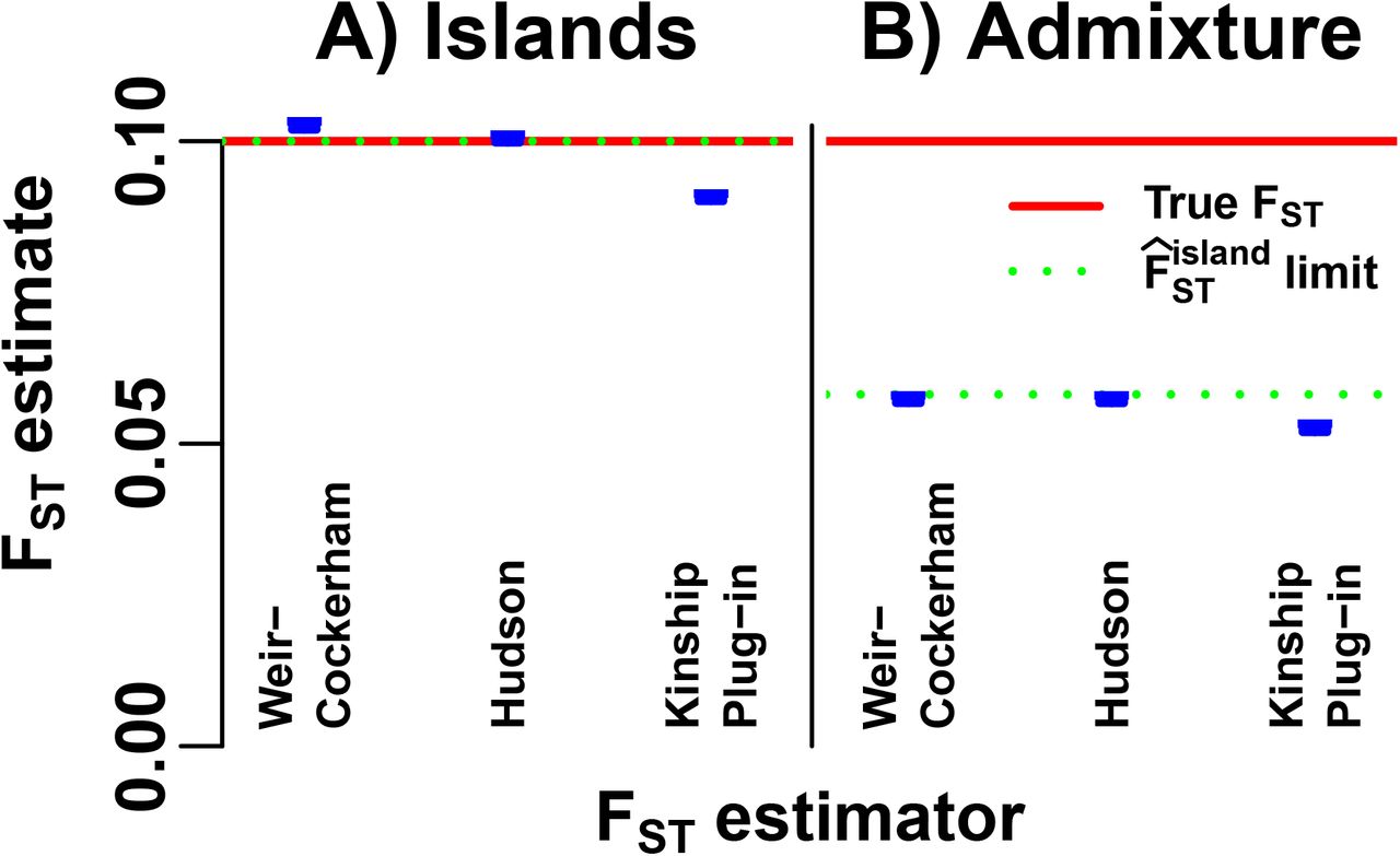
The WC, Hudson, and “kinship plug-in”  estimator of Eq. (30), are evaluated on simulated genotypes from our two models (Fig. 2): A) the island model assumed by the Hudson FST estimator, and B) our admixture scenario, a non-island model constructed so
  . The estimator limit of Eq. (15) (green dotted line) overlaps the true FST (red dashed line) in (A) but not (B). Estimates (blue) include 95% prediction intervals (too narrow to see) from 39 independently-simulated genotype matrices for each model (Appendix G).
To apply the WC and Hudson estimators to the admixture model, individuals are assigned to “populations” grouping by their maximum admixture proportions (Fig. 3D). Both WC and Hudson estimates are smaller than the true FST by nearly half, as predicted by the limit of  of Eq. (15) (Fig. 4C). By construction, the plug-in
  also has a large relative bias of about s = 50%; remarkably, the WC and Hudson estimators suffer from comparable biases. Thus, the island model corrections of the WC and Hudson estimators are insufficient for estimating FST in our admixture scenario.
6.3 Evaluation of individual-level pairwise FST estimators
Fig. 5A shows the matrix of true individual-level pairwise FST values, Fjk, for every pair of individuals in our simulation. Fjk is a distance between pairs of individuals, with Fjk = 0 for pairs from the same population and increasing values for more distant population pairs. Larger  lead to smaller Fjk (see Eq. (16)), hence the
  (Fig. 2B) and Fjk (Fig. 5A) matrices are negatively correlated.

Consistency of our individual-level pairwise FST estimators is demonstrated in our admixture simulation. Plots show n = 1000 individuals along both axes, and color corresponds to Fjk between individuals j and k. A) True pairwise FST matrix. The pairwise FST measures the mean differentiation of each pair of individual from their last common ancestor, and is negatively correlated with coancestry. B) Estimate from IAFs. C) Estimate from genotypes.
Both of our consistent Fjk estimators perform well, using IAFs (Eq. (16), Fig. 5B) and genotypes (Eq. (17), Fig. 5C). Estimates from genotypes have a greater root-mean-squared error (RMSE, 3.43% relative to the mean Fjk) than the estimates from true IAFs (RMSE of 0.319%).
6.4 Evaluation of the standard kinship estimator
Our admixture simulation illustrates the distortions of the kinship estimator  of Eq. (23). The limit of Eq. (23) has a fixed bias if
  for all j. For that reason, we chose
  that vary per u (Fig. 3A), which causes large differences in
  per j and large distortions in
  .
.
Compared to the true  (Fig. 6A, where
  are plotted along the diagonal),
  are very distorted, with an abundance of
  cases, negative estimates (blue in Fig. 6B), but remarkably also cases with
  (top left corner of Fig. 6B). Our ratio-of-means estimator
  agrees with the limit of Eq. (24) (Fig. 6C), which an RMSE of 2.14% relative to the mean
  . In contrast, mean-of-ratios estimates have an RMSE of 10.77% from the limit of Eq. (24) (not shown). The distortions are similar for the estimator that uses IAFs of Eq. (29) (not shown), with reduced RMSEs from its limit of 0.32% and 8.82% for the ratio-of-means and mean-of-ratios estimates, respectively.

Bias for the “standard” kinship coefficient estimator is illustrated in our admixture simulation. Plots show n = 1000 individuals along both axes, and color corresponds to  between individuals j and k, except the diagonal (j = k) shows
  for a comparable scale. A) True kinship matrix. B)
  of Eq. (23) estimated from simulated genotypes. C) Theoretical limit of
  estimator of Eq. (24) as the number of independent SNPs goes to infinity.
6.5 Evaluation of plug-in and adjusted FST estimators
We illustrate the behavior of our plug-in and adjusted FST estimators using our admixture simulation. We tested IAF (Fig. 7A) and genotype (Fig. 7B) versions of our estimators. The unadjusted plug-in  of Eq. (31) is severely biased (blue), by construction, and matches the calculated limit for IAFs and genotypes (green dotted lines in Fig. 7, which are close because
  ). We also tested the two consistent “adjusted” estimators
  and
and  of Eqs. (32) and (36), which estimate FST quite well (blue predictions overlap the true FST red dashed line in Fig. 7). However,
  and
and  are oracle methods, since they require parameters
  that are not known in practice.

The plug-in and adjusted FST estimators are evaluated using our admixture simulation. All adjusted estimators are “oracle” methods, since  , s are usually unknown. A) Estimation from IAFs: “plug-in” estimator is
  from Eq. (31); “Adj.
  ” is
” is  from Eq. (32); “Adj. s” is
  from Eq. (36). B) For genotypes, the “plug-in” estimator is given in Eq. (30), and the adjusted estimators use
  rather than
  . Lines: true FST (red dashed line), limits of biased estimators (green dotted lines, which differ slightly per panel). Estimates (blue) include 95% prediction intervals (too narrow to see) from 39 independently-simulated genotype matrices for our admixture model (Appendix G).
Prediction intervals were computed from estimates over 39 independently-simulated IAF and genotype matrices (Appendix G). Estimator limits are always contained in these intervals, which holds since the number of independent SNPs (m = 300, 000) is sufficiently large. Estimates that use genotypes have wider intervals than estimates from IAFs; however, IAFs are not known in practice, and use of estimated IAFs might increase noise. Genetic linkage, not present in our simulation, will also increase noise in real data.
7 Analysis of 1000 Genomes Project populations
We analyze 1000 Genomes Project (TGP) populations [20] with the Hudson FST estimator for two populations and our individual-level FST estimator,  , of Eq. (17). We focus on
  since it is currently our only consistent estimator for arbitrary population structures. We analyze the 20,417,698 biallelic SNP ascertained in YRI from autosomal chromosomes in the final “phase 3” data on the TGP website (dated 2013-05-02). Of these, 14,145,759 SNPs are polymorphic in the Hispanic populations and 8,932,115 in the European populations discussed below. Individuals in these data are roughly locally outbred and locally unrelated [20], which is the only requirement for the consistency of
  estimated from genotypes.
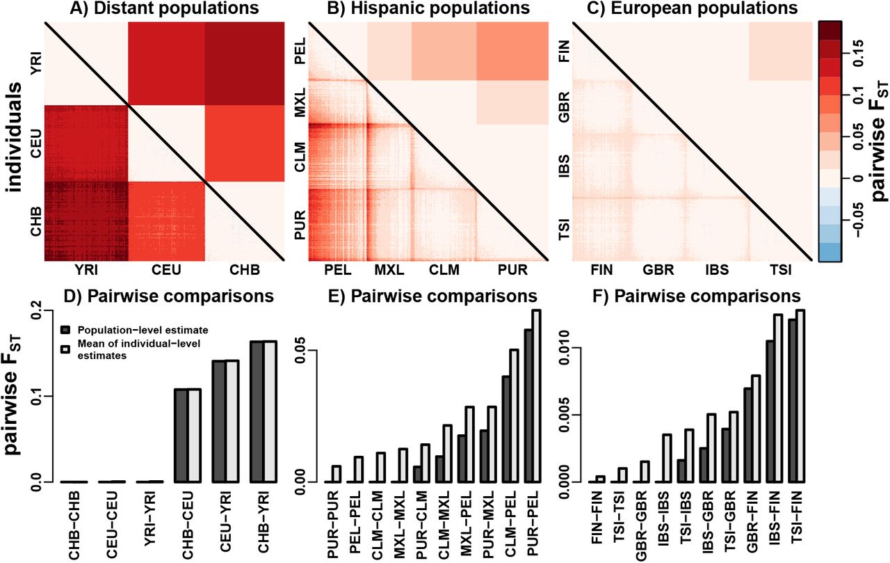
First we focus on YRI, CEU, and CHB, which were analyized previously [4]. These population pairs are geographically distant, so the island model is more likely to fit well. Indeed, Hudson estimates are relatively close to  (compare upper and lower triangle of Fig. 8A). In other words, the structure within populations is dwarfed by the structure between populations. A direct comparison to the Hudson estimates is given by
  of Eq. (19), which averages
  across populations for j ∈ Su and k ∈ Sv. We find good agreement between Hudson estimates and
  , corroborating a good fit of the island model (Fig. 8D).
Comparison of “population-level” Hudson FST estimates (upper triangle of A-C) and our “individual-level” pairwise FST estimates (lower triangle of A-C). All SNPs were ascertained in YRI. In (A-C), individuals in each population were ordered using their individual-level pairwise FST submatrix and the “seriate” function of R package “seriation” with default options. A) Geographically distant populations (310 individuals) are well approximated by the island model. YRI: Yoruba in Ibadan, Nigeria; CEU: Utah Residents with Northern and Western European Ancestry; CHB: Han Chinese in Beijing, China. B) Hispanic populations (347 individuals) are structured due to variable individual admixture proportions from primarily Native American, European, and African populations. PEL: Peruvians from Lima, Peru; MXL: Mexican Ancestry from Los Angeles USA; CLM: Colombians from Medellin, Colombia; PUR: Puerto Ricans from Puerto Rico. C) European populations (404 individuals) are closely related and geographically proximal. TSI: Toscani in Italy; FIN: Finnish in Finland; GBR: British in England and Scotland; IBS: Iberian Population in Spain. D-F) Populationlevel (Hudson) FST estimates are uniformly smaller than  (see text) for all pairs of populations.
Next, we analyze the four Hispanic populations in the TGP: PEL, MXL, CLM, and PUR. Hispanic individuals are admixed primarily from Native American, European, and African super-populations. Each of these populations is structured, a consequence of variable individual admixture proportions [27], so pairwise comparisons are poorly fit by the island model. The complex structure of these populations is confirmed by  , finding many individuals that have closer relatives from other populations compared to some individuals from the same population (lower triangle of Fig. 8B). Here we find that
  are always larger than their corresponding Hudson estimates (Fig. 8E). The largest proportional discrepancy is between PUR and CLM, whose Hudson estimate is 40% of
  . The Hudson estimator is solely a function of average allele frequencies and sample sizes per population (Appendix B), so it averages out the substructure within populations, explaining the smaller estimates observed relative to
  .
.
Lastly, we analyze four European populations: FIN, GBR, IBS, and TSI. We exclude CEU due to its similarity to GBR and because it was not sampled within Europe. The structure of European populations was previously found to disagree with the island model [44]. We confirm structure within these populations, although differentiation is much smaller here (Fig. 8C). Notably, proportional differences between Hudson and  are as large within Europe (Fig. 8F) as in the Hispanic populations (Fig. 8E). The largest proportional difference was between TSI and IBS, whose Hudson estimate is 41% of
  . Thus, our individual-level pairwise FST estimator,
  , detects structure that is missed by island model estimators.
8 Discussion
We investigated the most commonly utilized estimators of FST and kinship, both of which can be derived using the method of moments (Fig. 1). We determined the bias of these estimators under models of arbitrary population structure. We calculated the bias that occurs in the FST estimator when the island model assumption is violated. This bias is present even when individual-specific allele frequencies are known without error. We also showed that the kinship estimator is biased when the population is structured (particularly when the average kinship is of a similar magnitude to the true kinship coefficient), and that the bias may be different for each pair of individuals.
Use of island model FST estimators requires taking certain precautions, as exemplified in the Hudson FST estimator work [4]. First, the Hudson estimator is given for two populations only, since two panmictic populations are always independent relative to their last common ancestor population. Second, only geographically distant population pairs were compared [4], which appear internally unstructured relative to the structure between populations. However, FST is often estimated between closely related populations, for example, within Mexico [21], the United Kingdom [22], and between contemporary and archaic European [23] and Eurasian populations [24]. These geographically close populations are more likely to have comparable structure within and between populations, a case where Hudson underestimates differentiation, just as in the Hispanic and European populations in Fig. 8. Our analyses highlight the need for new tools that measure differentiation in complex population structures.
We have shown that the misapplication of existing FST estimators on non-island population structures may lead to estimates that approach zero even when the true generalized FST is large. Weir-Cockerham [3] and Hudson [4] FST estimates in our admixture simulation are biased by nearly a factor of two (Fig. 4). These estimators were derived assuming independent populations, so the observed biases arise from their misapplication to non-island populations. Nevertheless, natural populations often do not adhere to the island model, particularly human populations [44–46].
The kinship coefficient estimator we investigated is often used to control for population structure in GWAS and to estimate genome-wide heritability [9, 10, 13–18]. While this estimator was known to be biased [10, 18], no closed form limit had been calculated until now. We found that kinship estimates are biased downwardly on average, but bias also varies for every pair of individuals (Fig. 1, Fig. 6). Thus, the use of these distorted kinship estimates may be problematic in GWAS or estimating heritability, but to what extent remains to be determined.
We developed a theoretical framework for assessing these genome-wide ratio estimators of FST and kinship. We proved that common ratio-of-means estimators converge almost surely to the ratio of expectations for infinite independent SNPs (Appendix A.1). Our result justifies approximating the expectation of a ratio-of-means estimator with the ratio of expectations [3–5]. However, mean-of-ratios estimators may not converge to the ratio of expectations for infinite SNPs. Mean-of-ratios estimators are potentially asymptotically unbiased for infinite individuals, but it is unclear which estimators have this behavior. We found that the ratio-of-means kinship estimator had much smaller errors from the ratio of expectations than the more common mean-of-ratios estimator, whose convergence value is unknown. Thus, we recommend ratio-of-means estimators, whose asymptotic behavior is well understood.
The Hudson estimator is a consistent estimator of the pairwise FST for two populations [4], which is reported often [21–24, 45, 47]. We derived a consistent estimator of the individual-level pairwise FST, Fjk, which extends the previous pairwise FST to individuals [25]. However, kinship or FST estimates for more than two individuals cannot be recovered from Fjk estimates. Conceptually, kinship and FST are in terms of a single ancestral population T, whereas each Fjk is relative to a jointly local population Ljk that varies per (j, k) pair (see Eq. (5)). Practically, there is loss of information since Fjj = 0 for every j by definition: for n individuals, there are n more  than Fjk parameters. We used our Fjk estimator to identify structure with individual resolution in 1000 Genomes Project populations (Fig. 8).
Accurate estimation of generalized FST and kinship coefficients in arbitrary population structures will require further innovations, and the results provided here may be useful in leading to more robust estimators in the future. This, in particular, is the topic we tackle in the next paper in this series [32].
Appendices
A Accuracy of ratio estimators
A.1 Almost sure convergence of ratio-of-means estimators with independent and uniformly bounded terms
Here we prove that  , where
  and
and  give the ratio-of-means estimator described in the main text. It suffices to prove
  and
and  , from which the result follows using the continuous mapping theorem [48, 49]. The proof for
  follows, which applies analogously to
  . Our ai are independent but not identically distributed, since they depend on
  that varies per SNP, so the standard law of large numbers does not apply to Âm. We show almost sure convergence using Kolmogorov’s criterion for the Strong Law of Large Numbers [50], which is satisfied for bounded Var(ai). Since |ai| ≤ C ≤ ∞ for all i and some C (see main text), then
  , so Var(ai) ≤ C2. Therefore,
  , as desired.
A.2 Order of error of expectations
The error of the ratio of expectations from the expectation of the ratio is given by
 which follows from Cov(X, Y) = E[XY] − E[X] E[Y] [51] and expanding the covariance. Previous work on ratio estimators [35, 51] assumes IID ai and bi, which does not hold for SNPs. Assuming independent SNPs (Cov(ai, aj) = 0 for i ≠ j) and large m so
  is practically independent of any given ai and bj, then
 Since ai, bi are bounded, | Cov(ai, bi) | ≤ C2 for the same C of the previous section, so
 holds for some large enough m and C. Hence
  is as for standard ratio estimators [35].
B Generalized Hudson FST estimator
The Hudson FST estimator compares two populations [4]. We generalize this estimator for n independent populations, where FST equals the mean pairwise FST for every pair of populations. We average numerators and denominators of the pairwise estimator before computing the ratio. Let j index the n populations, nj be the number of individuals sampled from j, and  be the sample allele frequency in j for SNP i, then
 which consistently estimates FST in island models.
C Derivation of method of moment estimators
C.1 FST island model estimator
Assuming the coancestry model of Eqs. (6) and (7) for islands ( for j ≠ k), the first and second moments of the IAFs are:


 appears by averaging Eq. (C.2) over j:
 Since Eq. (C.1) has the same value for every j, and Eq. (C.3) as well for every j ≠ k, we average these to reduce estimation variance. The results are in terms of
  :
:

 FST also appears in Eq. (C.6) because j = k terms are introduced in the double sum. Subtracting Eq. (C.4) and Eq. (C.6) in turn from Eq. (C.5) results in:
 To reduce variance further, we average across SNPs, giving
 where
where  . Eliminating
  and solving for FST in this system of equations results in the following FST estimator:
 This estimator is simplified noting that
  appears in the IAF sample variance,
 so substituting it into Eq. (C.7) recovers Eq. (14) as desired:

C.2 Standard kinship estimator
Here we assume the kinship model of Eqs. (1) and (2). Since Eq. (1) is the same for all individuals j, we average these first moments to reduce variance:
 Each
Each  appears once per (j, k) pair in Eq. (2), recast here in terms of the sample covariance:
 Variance in the kinship estimate is reduced by averaging across SNPs, yielding:
 The resulting estimator of
  is
is
 which is plugged into Eq. (C.8) and then
  is solved for, recovering Eq. (23) as desired:

D Mean coancestry bounds
Here we prove that, for any weights such that  ,
,
 holds, and for uniform weights
  also holds. Furthermore,
  holds iff
  for all (j, k), and
  holds for island models.
The Cauchy-Schwarz inequality for covariances implies  . Therefore,
 where the second inequality follows from Jensen’s inequality, since x2 is a convex function. Since
  , then FST ≤ 1 as well. Equality in the second bound requires
  for all j, and equality in the first bound requires
  , so that
  requires
  for all (j, k). Since all wj,
  , then
 where the second inequality follows from dropping j ≠ k terms from the double sum of
  . The case
  gives
gives  , with equality for island models by construction.
E Moments of estimator building blocks
Here we calculate first and some second moments for “building block” quantities that recur in our estimators, particularly terms involving xij and  , and which enable us to calculate the limits of our estimators. Below are examples for genotypes, which follow from Eqs. (1) and (2); calculations for IAFs follow analogously from Eqs. (6) and (7) (not shown).

F Admixture and island model simulations
F.1 Construction of population island allele frequencies
We simulate K = 10 population islands and m = 300, 000 independent SNPs. Every SNP i draws  . We set
  , where τ ≤ 1 tunes FST. For the island model,
  , so
, so  gives the desired FST (τ ≈ 0.18 for FST = 0.1). For the admixture model, τ is found numerically (τ ≈ 0.90 for FST = 0.1; see last subsection). Lastly,
  are drawn from the Balding-Nichols distribution [41]:

F.2 Random island sizes
We randomly generate samples sizes r = (ru) for K islands and  individuals, as follows. First, draw x ~ Dirichlet (1, …, 1) of length K and r = round(nx). While
  , draw a new r, to prevent small islands (they do not occur in real data). Lastly, while
  , a random u is updated to ru ← ru + sgn(δ), which brings δ closer to zero. The resulting r is as desired. Weights for individuals j in Su are
  so the generalized FST matches
  from the island model, which Hudson estimates [25].
F.3 Admixture proportions from 1D geography
We construct qju resulting from random-walk migrations along a one-dimensional geography. Let xu be the coordinate of intermediate population u and yj the coordinate of a modern individual j. We assume qju is proportional to f (|xu − yj|), or
 where f is the Normal density function with μ = 0 and tunable σ. The Normal density models random walks, where σ sets the spread of the populations (Fig. 6). Our simulation uses xu = u and
  , so intermediate population span [1, K] and individuals span
  . For the WC and Hudson FST estimators, individual j is assigned to the subpopulation Su with the largest qju (Fig. 3D); thus these subpopulations have equal sample size, so
  is appropriate.
F.4 Choosing σ and τ
Here we find values for σ (controls qjk) and T (scales  ) that give
  and FST = 0.1 in the admixture model. We previously found that
  and
and  holds for the BN-PSD model [25]. In our simulation,
  and
and  hold, so
  and
and  . Therefore,
 depends only on σ. A numerical root finder finds that σ ≈ 1.78 gives
  . For fixed qju,
 where FST is the desired value. FST = 0.1 is achieved with τ ≈ 0.901.
G Prediction intervals of FST estimators
Prediction intervals with α = 95% correspond to the range of n = 39 independent FST estimates. In the general case, n independent statistics are given in order X(1) < … < X(n). Then I = [X(j), X(n+1−j)] is a prediction interval with confidence  [52]. In our case, j = 1 and n = 39 gives α = 0.95, as desired. Each estimate was constructed from simulated data with the same dimensions and structure as before (fixed
  and qju; fixed sample sizes too for island models), but with
  , πij, xij drawn anew.
References


