

Abstract
A number of open questions in human evolutionary genetics would become tractable if we were able to directly measure evolutionary fitness. As a step towards this goal, we developed a method to test whether individual genetic variants, or sets of genetic variants, currently influence viability. The approach consists in testing whether the frequency of an allele varies across ages, accounting for variation in ancestry. We applied it to the Genetic Epidemiology Research on Aging (GERA) cohort and to the parents of participants in the UK Biobank. In the GERA cohort, the top signal is the APOE ε4 allele (P < 10−15), whereas in the UK Biobank, the strongest signals are detected in males only, and are for variants near CHRNA3 (P~4×10⁻⁸) as well as set of genetic variants that influence heart disease and lipid levels. We suggest that gene-by-environment interactions have altered the genetic architecture of viability in these two cohorts.
Introduction
A number of central questions in evolutionary genetics remain open, in particular for humans. Which types of variants affect fitness? Which components of fitness do they affect? What is the relative importance of viability and balancing selection in shaping genetic variation? Part of the difficulty is that our understanding of selection pressures acting on the human genome is based either on experiments in fairly distantly related species or cell lines, necessarily biased towards cases with simpler genetic architectures, or on indirect statistical inferences from patterns of genetic variation (Sabeti et al. 2006; Nielsen et al. 2007; Fu and Akey 2013).
The statistical inferences rely on patterns of genetic variation in present day samples (or very recently, in ancient samples (Mathieson et al. 2015)) to identify regions of the genome that appear to carry the footprint of positive selection (Nielsen et al. 2007). For example, a commonly used class of methods asks whether rates of non-synonymous substitutions between humans and other species are higher than expected from putatively neutral sites, in order to detect recurrent changes to the same protein (Yang and Bielawski 2000). Another class instead relies on polymorphism data and looks for various footprints of adaptation involving single changes of large effect (Maynard Smith and Haigh 1974). These approaches detect adaptation over different timescales and, likely as a result, suggest quite distinct pictures of human adaptation (Sabeti et al. 2006). For example, approaches that are sensitive to selective pressures acting over millions of years have identified individual chemosensory and immune-related genes (e.g., (Nielsen et al. 2005)). In contrast, approaches that contrast patterns in different human populations and are most sensitive to selective pressures active over thousands or tens of thousands of years revealed strong selective pressures on individual genes that influence human pigmentation (e.g., (Field et al. 2016; Williamson et al. 2007; Voight et al. 2006)), diet (Bersaglieri et al. 2004; Tishkoff et al. 2007; Perry et al. 2007), as well as sets of variants that shape height (Turchin et al. 2012; Robinson et al. 2015; Berg and Coop 2014). Even more recent still, studies of contemporary populations have suggested that natural selection has influenced life history traits like age at first childbirth as well as educational attainment over the course of the last century (Stearns et al. 2010; KAar et al. 1996; Byars et al. 2010; Milot et al. 2011; Tropf et al. 2015; Beauchamp 2016).
Because these approaches are designed (either explicitly or implicitly) to be sensitive to a particular mode of adaptation, they provide a partial and potentially biased picture of what variants in the genome are under selection. In particular, most have much higher power to adaptations that involve strongly beneficial alleles that were rare in the population when first favored and will tend to miss selection on standing variation or adaptation involving many loci with small beneficial effects (e.g., (Przeworski, Coop, and Wall 2005; Pennings and Hermisson 2006; Teshima, Coop, and Przeworski 2006; Coop et al. 2009)). Moreover, even where these methods identify a beneficial allele, they are not informative about possible fitness trade-offs between sexes or across ages.
Here, we aim to develop a more direct and, in principle, comprehensive way to study adaptation in humans, focusing on current viability selection. Similar to the approach that Alison took in comparing frequencies of the sickle cell allele in newborn and adults living in malarial environments (Allison 1964), our approach is to directly observe the effects of genotypes on survival by taking advantage of the recent availability of genotypes from a large cohort of individuals of different ages. Specifically, we test for differences in the frequency of an allele across individuals of different ages, correcting for changes in ancestry and possible batch effects. This approach is sensitive to variants that impact survival to a given age. Any genetic variant that affects survival by definition has a fitness cost, even if the cost is too small to be effectively selected against (which depends on the effective population size, the age structure of the population and the age at which the variant exerts its effects (Charlesworth 1994)). Of course a genetic variant can influence fitness without influencing survival, through effects on reproduction or inclusive fitness. Thus, our approach considers only one of the components of fitness that are likely important for human adaptation.
As a proof of principle, we apply our approach to two recent datasets: to 57,696 individuals of European ancestry from the Resource for Genetic Epidemiology Research on Aging (GERA) Cohort (Banda et al. 2015; Kvale et al. 2015) and, by proxy (Joshi et al. 2016; Pilling et al. 2016), to the parents of 95,513 individuals of European ancestry surveyed as part of the UK Biobank (UK Biobank). We do so for individual genetic variants, then jointly for sets of variants previously found to influence one of 40 polygenic traits (Pickrell et al. 2016).
Results
Our method for testing for differences in allele frequencies across age bins
If a genetic variant does not influence viability, its frequency should be the same in individuals of all ages. We therefore test for changes in allele frequency across individuals of different ages, while accounting for systematic differences in the ancestry of individuals of different ages (for example, as a result of migration patterns over decades) and genotyping batch effects. We use a logistic regression model in which we regress each individual’s genotype on their age bin, their ancestry as determined by principal component analysis (PCA) (Figure S1), and the batch in which they were genotyped (see Materials and Methods for details). In this model, we treat age bin as a categorical variable; this allows us to test for a relationship between age and the frequency of an allele regardless of the functional form of this relationship. We also test a model with an interaction between age and sex, to assess whether a variant affects survival differently in the two sexes.
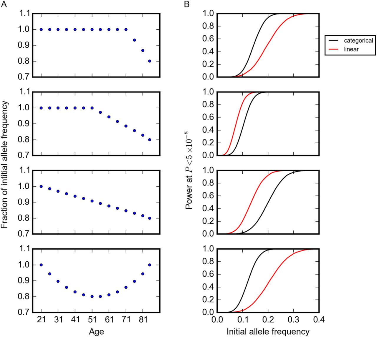
We first evaluated the power of this method using simulations. We considered three possible trends in allele frequency with age: (i) a constant frequency up to a given age followed by a steady decrease, i.e., a variant that affects survival after a given age (e.g., variants contributing to late-onset disorders), (ii) a steady decrease across all ages for a variant with detrimental effect throughout life, and (iii) a U-shape pattern in which the allele frequency decreases to a given age but then increases, reflecting trade-offs in the effects at young and old ages, as hypothesized by the antagonistic pleiotropy theory of aging (Williams 1957) or as may be seen if there are protective alleles whose effects are visible late in life (Bergman et al. 2007) (Figure 1). In all simulations, we used sample sizes and age distributions that matched the GERA cohort (Figure S2). For simplicity, we also assumed no population structure or batch effects across age bins (Materials and Methods). For all trends, we set a maximum of 20% change in the allele frequency from the value in the first age bin (Figure 1).

Power of the model to detect changes in allele frequency with age. (A) Trends in allele frequency with age considered in simulations. The y-axis indicates allele frequency normalized to the frequency in the first age bin. (B) Power to detect the trends in (A) at P < 5×10⁻⁸, given the sample size per age bin in the GERA cohort (Figure S2 and total sample size of 57,696). Shown are results using models with age treated as a categorical (black) or an ordinal (red) variable, assuming no change in population structure and batch effects across age bins. The curves show simulation results sweeping allele frequency values with an increment value of 0.001 (1000 simulations for each allele frequency) smoothed using a Savitzky-Golay filter using the SciPy package (Jones, Oliphant, and Peterson 2001).
Because of the age distribution of individuals in the GERA cohort (Figure S2), our power to detect the trend is greater when most of the change in allele frequency occurs at middle ages (Figure 1). For example, for an allele with an initial allele frequency of 15% that begins to decrease in frequency among individuals at age 20, age 50, or age 70 years, there is around 20%, 90% and 60% power, respectively, to detect the trend at P < 5×10⁻⁸, the commonly-used criterion for genome-wide significance (Pe’er et al. 2008). We also experimented with a version of the model where the age bin is treated as an ordinal variable; as expected, this model is more powerful if there is a linear relationship between age and allele frequency (Materials and Methods). Since in most cases, we do not know the functional form of the relationship between age and allele frequency a priori, we used the categorical model for all analyses, unless otherwise noted.
In the UK Biobank, all individuals were 45-69 years old at enrollment, so the age range of the participants is restricted and our method has low power. However, the UK Biobank participants reported the age at death of their parents; following two recent studies (Joshi et al. 2016; Pilling et al. 2016), we therefore used these values (when reported) instead in our model. In this situation, we are testing for correlations between an allele frequency and the age at which the father or mother died. This approach obviously comes with the caveat that children inherit only 50% of their genome from each parent and so power is reduced (e.g., (Liu, Erlich, and Pickrell 2016)). Further, the patterns expected when considering individuals who have died differ subtly from those generated among surviving individuals. Notably, when an allele begins to decline in frequency starting at a given age (Figure 1A), there should be an increase in the allele frequency among individuals who died at that age, followed by a decline in frequency, rather than the steady decrease expected among surviving individuals (Figure S3, see Materials and Methods for details).
We also adapted this model to allow us to test for changes in frequency at sets of genetic variants. Many phenotypes of interest, from complex disease risk to anthropomorphic traits such as age of menarche, are polygenic (Visscher et al. 2012; He and Murabito 2014). If a polygenic trait has an effect on fitness, either directly or indirectly (i.e., through pleiotropic effects), the individual loci that influence the trait may be too subtle in their survival effects to be detectable with current sample sizes. We therefore investigated whether there is a shift across ages in sets of genetic variants that were identified as influencing a trait in genome-wide association studies (GWAS) (Table S1). Specifically, for a given trait, we calculated a polygenic score for each individual based on trait effect sizes of single variants previously estimated in GWAS and then test whether the scores vary significantly across age bins (see Materials and Methods for details). These scores are calculated under an additive model, which appears to provide a good fit to GWAS data (Cantor, Lange, and Sinsheimer 2010). If a polygenic trait is under stabilizing selection (e.g., human birth weight (Karn and Penrose 1951)), i.e., an intermediate polygenic score is optimal, no change in the mean value of polygenic score across different ages is expected. However, if extreme values of a trait are associated with lower chance of survival, the spread of the polygenic scores should decrease with age. To consider this possibility, we tested whether the squared difference of the polygenic scores from the population mean varies significantly across age bins (see Materials and Methods for details).
Testing for changes in allele frequency at individual genetic variants
We first applied the method to the GERA cohort, using 9,010,280 filtered genotyped and imputed autosomal single-nucleotide polymorphisms (SNPs). We focused on a subset of filtered 57,696 individuals confirmed to be of European ancestry by PCA (see Materials and Methods, Figures S4 and S5). The ages of these individuals were reported in bins of 5 year intervals (distribution shown in Figure S2). We tested for significant changes in allele frequencies across these bins. For each SNP, we obtained a P value comparing a model in which the allele frequency changes with age to a null model (quantile-quantile plot shown in Figure S6A). All variants that reached genome-wide significance (P < 5×10⁻⁸) reside on chromosome 19 near the APOE gene (Figure 2A and Figure S7). This locus has previously been associated with longevity in multiple studies (Christensen, Johnson, and Vaupel 2006; Murabito, Yuan, and Lunetta 2012). The ε4 allele of the APOE gene is known to increase the risk of late-onset Alzheimer’s disease (AD) as well as of cardiovascular diseases (Corder et al. 1993; Bennet et al. 2007). We observed a monotonic decrease in the frequency of the T allele of the ε4 tag SNP rs6857 (C, protective allele; T, risk allele) beyond the age of 70 years old (Figure 2B). This trend is observed for both the heterozygous and homozygous risk variants (Figure S8), and for both males and females (Figure S9). No variant reached genome-wide significance testing for age by sex interactions (quantile-quantile plot shown in Figure S6B).

Testing for the influence of single genetic variants on age-specific mortality in the GERA cohort. (A) Manhattan plot for change in allele frequency with age P values. Red line marks the P = 5×10⁻⁸ threshold. (B) Allele frequency trajectory of rs6857, a tag SNP for APOE ε4 allele, with age. Data points are mean frequency of the risk allele within 5-year interval age bins (and 95% confidence interval), with the center of the bin indicated on the x-axis. Bins with ages below 36 years are merged into one bin because of the relatively small sample sizes per bin. The dashed line shows the expected frequency based on the null model accounting for confounding batch effects and changes in ancestry (see Materials and Methods). In orange are the mean age of onsets of Alzheimer’s disease for carriers of 0, 1 or 2 copies of the APOE ε4 allele (Corder et al. 1993).
We further investigated the trends in frequency with age for the other two major APOE alleles defined by rs7412 and rs429358 SNPs: ε2 (rs7412-T, rs429358-T) and ε3 (rs7412-C, rs429358-T), while ε4 is (rs7412-C, rs429358-C) (Liu et al. 2013). Unlike the ε4 allele, ε2 carriers are suggested to be at lower risk of Alzheimer’s disease, cardiovascular disease, and mortality relative to the ε3 carriers (Liu et al. 2013; Christensen, Johnson, and Vaupel 2006). We focused on a subset of 38,703 individuals with unambiguous counts of each APOE allele. There is a significant change in the frequency of the ε4 allele with age in this subset (P~6×10⁻¹²), similar to the trend observed for the tag SNP rs6857 (Figure S10). The ε3 allele showed the reverse trend, with a significant, monotonic increase in frequency beyond age of 70 years old (P~2×10⁻⁸) (Figure S10). The enrichment of the ε3 allele in elderly individuals can be explained by the corresponding depletion of the ε4 allele, however, so does not necessarily imply an independent, protective effect of ε3. The frequency of the ε2 allele did not change significantly with age (P~0.2), which may reflect low power for the allele frequency of ~0.06 (Figure S10).
We considered the possibility that some unobserved confounding variable was driving the strength of this signal at APOE. Since we observe two genotyped SNPs with signals similar to rs6857 within the locus, genotyping error seems unlikely to be driving the pattern (Figure S7). Another concern might be a form of ascertainment bias, in which individuals with Alzheimer’s disease are underrepresented in the Kaiser Permanente Medical Care Plan. However, there is no correlation in these data between the amount of time that an individual has been enrolled in this insurance plan and the individual’s APOE genotype (Figure S11). These observations, along with previously reported associations at this locus, argue that the allele frequency trends in Figure 2B are driven by effects of APOE genotype on mortality (or severe disability). Moreover, the effects that we identify are concordant with epidemiological data on the peak age of onset of Alzheimer’s disease given 0 to 2 copies of APOE ε4 (Corder et al. 1993). Thus, this case illustrates how our approach provides resolution about age effects of deleterious variants.
We estimated that we have ~93% power to detect the trend in allele frequency with age as observed for rs6857 (at a genome-wide significance level; see Materials and Methods). Using both versions of the model treating age bin as either a categorical or an ordinal variable, we have similar power to detect other potential trends considered in Figure 1, for variants as common as rs6857 and with similar magnitude of effect on survival. Yet across the genome, only APOE variants show a significant change in allele frequency with age for both versions of the model (Figure 2 and Figure S12), suggesting that there are few common variants in the genome with an effect on survival as strong as seen in APOE region.
We then turned to the UK Biobank data. We applied our method to individuals of European ancestry whose data passed our filters; of these, 88,595 had death information available for their father and 71,783 for their mother. We analyzed 590,437 genotyped autosomal variants, applying similar quality control measures as with the GERA dataset (see Materials and Methods). We tested for significant changes in allele frequencies with father’s age at death and mother’s age at death stratified in eight 5-year interval bins (quantile-quantile plots shown in Figure S13).
Consistent with recent studies (Joshi et al. 2016; Pilling et al. 2016), the variants showing a genome-wide significant change in allele frequency with father’s age at death (P < 5×10⁻⁸) reside within a locus containing the nicotine receptor gene CHRNA3 (Figure 3A). The A allele of the CHRNA3 SNP rs1051730 (G, major allele; A, minor allele) has been shown to be associated with increased smoking quantity among individuals who smoke (Tobacco and Genetics Consortium 2010). We observed a linear decrease in the frequency of the A allele of rs1051730 throughout almost all age ranges (Figure 3B). This allele did not show a significant trend with age in GERA (P~0.45, Figure S14).
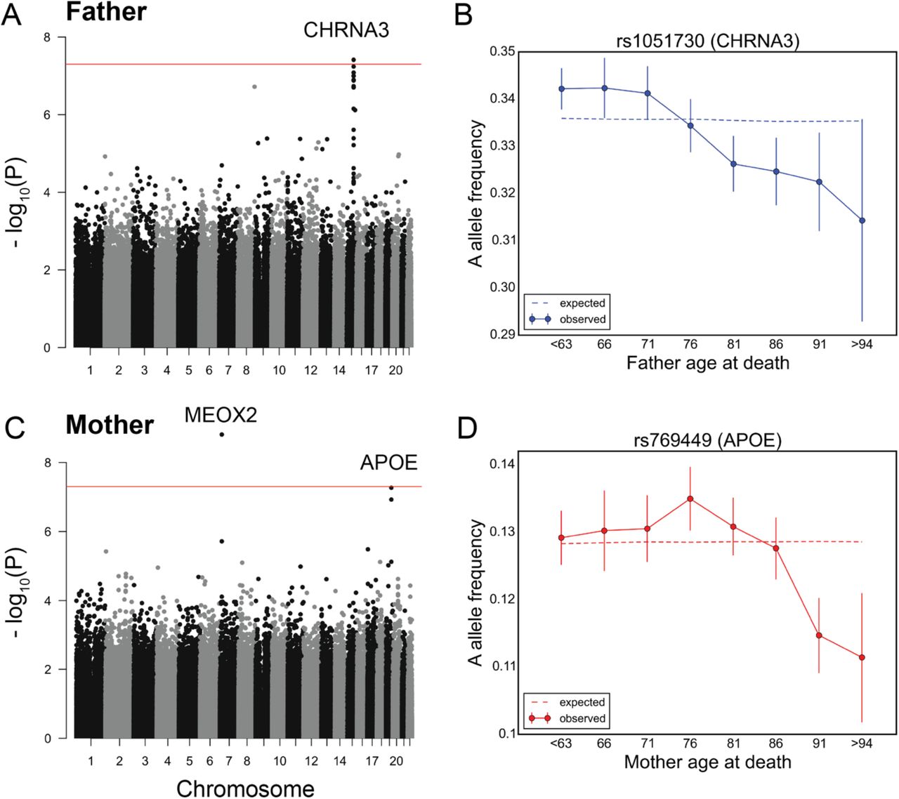
Testing for the influence of single genetic variants on age-specific mortality in the UK Biobank. (A) Manhattan plot for change in allele frequency with age at death of fathers P values. (B) Allele frequency trajectory of rs1051730, within CHRNA3 locus, with father’s age at death. (C) Manhattan plot for change in allele frequency with age at death of mothers P values. (D) Allele frequency trajectory of rs769449, within the APOE locus, with mother’s age at death. Red lines in (A) and (C) mark P = 5×10⁻⁸ threshold. Data points in (B) and (D) are mean frequency of the risk allele within 5-year interval age bins (and 95% confidence interval), with the center of the bin indicated on the x-axis. The dashed line shows the expected frequency based on the null model, accounting for confounding batch effects and changes in ancestry (see Materials and Methods).
For mother’s age at death, a SNP in a locus containing the MEOX2 gene reached genome-wide significance (Figure 3C). The C allele of rs4721453 (T, major allele; C, minor allele) increases in frequency in the age bin centered at 76 years old (Figure S15), i.e., there is an enrichment among individuals that died at 74 to 78 years of age, which corresponds to a deleterious effect of the C allele in this period. The trend is similar and nominally significant for other genotyped common SNPs in moderate linkage disequilibrium with rs4721453 (Figure S15). Also, the signal for rs4721453 remains nominally significant when using subsets of individuals genotyped on the same genotyping array: 44,552 individuals on the UK Biobank Axiom array (P~7×10⁻⁵) and 25,231 individuals on the UK BiLEVE Axiom array (P~10−4). These observations suggest that the result is not due to genotyping errors, but it is not reproduced in GERA (P~0.17, Figure S16) and so it remains to be replicated. APOE variants were among the top nominally significant variants (P < 10−7) (Figure 3C). At the APOE SNP rs769449 (G, major allele; A, minor allele), there is an increase in the frequency of A allele at around 70 years old before subsequent decrease (Figure 3D). This pattern is consistent with our finding in GERA (of a monotonic decrease beyond 70 years of age), considering the difference in patterns expected between allele frequency trends with age among survivors versus individuals who died (Figure S3).
We note that by considering parental age at death of the UK Biobank participants (as done also in (Joshi et al. 2016; Pilling et al. 2016)), we introduce a bias towards older participants (who are more likely to have deceased parents, Figure S17A). We confirmed that our top signals are not significantly affected by such potential bias, observing similar trends in allele frequency with parental age at death when conditioning on age of the participants (Figure 17B).
We further tested for trends in allele frequency with parental age at death that differ between fathers and mothers focusing on 62,719 individuals with age at death information for both parents. No SNP reached genome-wide significance level (Figure 18A). The rs4721453 near the MEOX2 gene and APOE variant rs769449 showed nominally significant sex effects (P~7×10⁻⁸ and P~2×10⁻³, respectively), with stronger effects in females (Figure 18B). Variants near the CHRNA3 locus were nominally significant when using the model with parental age at deaths treated as ordinal variables (rs11858836, P~6×10⁻⁴), with stronger effects in males (Figure 18B).
Testing for changes in allele frequency at trait-associated variants
We next applied our model to polygenic traits, rather than individual genetic variants. We focused on 40 polygenic traits, including disease risk and anthropomorphic traits of evolutionary importance such as age at menarche (AAM), for which a large number of common variants have been mapped in GWAS (see Table S1 for the list of traits and number of loci) (Pickrell et al. 2016). For each individual and each trait, we calculated a polygenic score, and then tested whether this polygenic score, or its squared difference from the mean in the case of stabilizing selection, differs among individuals in different age bins.
In the GERA cohort, no trait reached statistical significance, after accounting for multiple tests (Figure 4A). The strongest signal is a suggestive increase in the polygenic score for age at menarche in older ages (P~3.4×10⁻³, without correction for multiple testing; Figure 4B), consistent with epidemiological studies suggesting early puberty timing to be associated with various adverse health outcomes (Day, Elks, et al. 2015). We did not exclude males for analysis of age at menarche, because of the strong genetic correlation between the timing of puberty in males and females (Day, Bulik-Sullivan, et al. 2015). For disease traits potentially decreasing the chance of survival with increasing age, a monotonic decrease in polygenic score with age is plausible. Therefore, we also applied our version of the model with age treated as an ordinal variable, for which Alzheimer’s disease (AD) (excluding the APOE locus) showed the strongest signal (P~5.1×10⁻³, see Figure 4C), indicative of a decrease in chance of survival with increased genetic risk of AD (Figure 4D). No trait showed significant sex by age effect (Figure S19), or significant change in the squared difference of polygenic score from the mean with age (Figure S20).

Testing for the influence of set of trait-associated variants on age-specific mortality in the GERA cohort. (A) Quantile-quantile plots for change in the polygenic score of 40 traits (see Table S1) with age treated as a categorical variable. (B) Trajectory of polygenic score of age at menarche with age. (C) Same as (A) but with age treated as an ordinal variable. (D) Trajectory of polygenic score of Alzheimer’s disease (excluding the APOE locus) with age. The red lines in (A) and (C) indicate distribution of the P values under the null. See Table S2 for P values for all traits. Data points in (B) and (D) are mean polygenic score within 5-year interval age bins (and 95% confidence interval), with the center of the bin indicated on the x-axis. The dashed line shows the expected score based on the null model accounting for confounding batch effects and changes in ancestry.
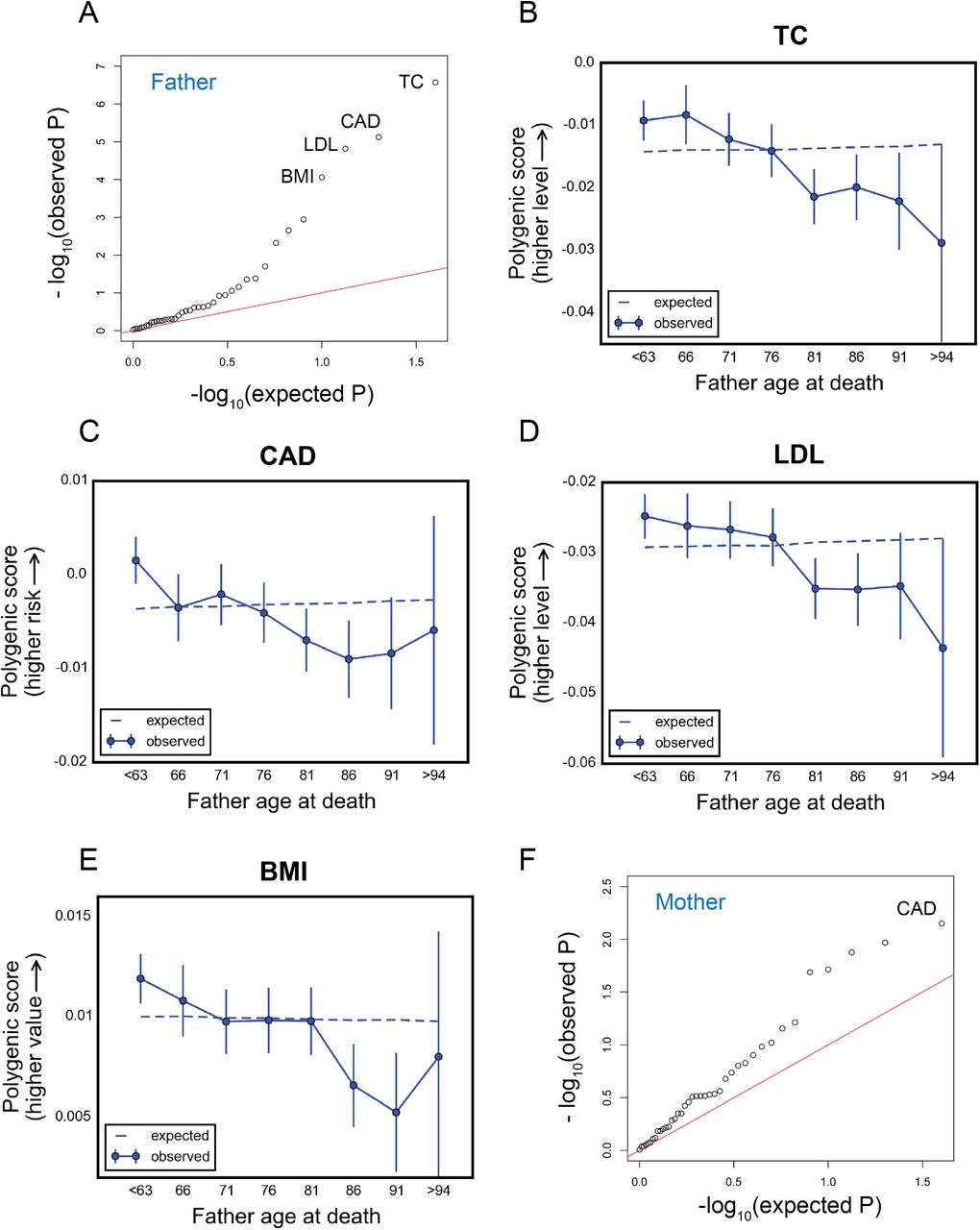
In the UK Biobank, consistent with two recent studies (Pilling et al. 2016; Marioni et al. 2016), several cardiovascular disease risk traits showed significant change in polygenic score with father’s age at death (Figure 5A): total cholesterol (P < 10−6), coronary artery disease (P < 10−5), low-density lipoproteins (P < 10−4), and body mass index (P < 10−4). The decline in score with age for these traits is approximately linear with age (Figure 5B-E). Testing for sex by age interaction, high-density lipoproteins showed the strongest signal, with seemingly distinct trends in males and females (P~3×10⁻⁴, Figures S21). Using the model with parental age at deaths treated as ordinal variables, total cholesterol showed stronger effects in males (P~7×10⁻⁴, Figures S21).

Testing for the influence of set of trait-associated variants on age-specific mortality in the UK Biobank. (A) Quantile-quantile plots for change in the polygenic score of 40 traits (see Table S1) with age at death of fathers of the UK Biobank participants. (B)-(E) Trajectory of polygenic score of traits showing significant change with age at death of fathers: total cholesterol (B), coronary artery disease (C), low-density lipoproteins (D), and body mass index (E). (F) Quantile-quantile plots for change in the polygenic score of traits in (A) with age at death of mothers of the UK Biobank participants. The red lines in (A) and (F) indicate the distribution of the P values under the null. See Table S2 for P values for all traits. Data points in (B)-(E) are mean polygenic score within 5-year interval age bins (and 95% confidence interval), with the center of the bin indicated on the x-axis. The dashed line shows the expected score based on the null model, accounting for confounding batch effects and changes in ancestry.
No trait showed significant change in polygenic score with mother’s age at death (Figure 5F). Also, no trait showed significant change in the squared difference of polygenic score from the mean with father’s or mother’s age at death (Figure S22). We confirmed that our different findings between the GERA cohort and the UK Biobank are not driven by using slightly different sets of trait-associated SNPs (considering that trait associated SNPs passing our filters were not identical), finding similar results when using SNPs that passed quality control steps in both datasets (Figure S23).
Discussion
We introduced a new approach to identify genetic variants that affect survival to a given age and thus to directly observe viability selection ongoing in humans. Attractive features of the approach include that we do not need to make a decision a priori about which traits matter to viability and focus not on an endpoint (e.g., lifespan) but on any shift in allele frequencies with age, thereby learning about the precise ages at which effects are manifest and possible differences between sexes.
To illustrate the potential of our approach, we performed a scan for genetic variants that impact age-specific mortality in the GERA and the UK Biobank cohorts. We only found a few variants, the majority of which were identified in previous studies. This result is in some ways expected: available data only provide high power to detect effects of common variants (>15-20%) on survival (Figure 1), yet if these variants were under viability selection, we would not expect them to be common, short of strong balancing selection due to trade-offs between sexes, ages or environments. As sample sizes increase, however, the approach introduced here should provide a much more comprehensive picture of viability selection in humans. To illustrate this point, we repeated our power simulation with 500,000 samples, and found that we should have high power to detect the trends for alleles at a couple percent frequency (Figure S24).
Already, however, this application raises a number of interesting questions about the nature of viability selection in humans. Notably, we discovered only a few variants influencing viability in the two cohorts, all of which exert their effect late in life. On first thought, it may be concluded that such variants are neutrally-evolving. We would argue that if anything, our findings of only a few common variants with effects on survival only late in life suggest the opposite: that even variants with late onset effects have been weeded out by purifying selection. Indeed, unless the number of loci in the genome that could give rise to such variants (i.e., the mutational target size) is tiny, other variants such as APOE must often arise. That they are not observed when we have very high power to detect them suggests they are kept at lower frequency by purifying selection. Why might they be selected despite affecting survival only at old ages? Possible explanation include that they decrease the direct fitness of males sufficiently to be effectively selected (notably given the large, recent effective population size of humans (Gazave et al. 2014)) or that they impact the inclusive fitness of males and females. If this explanation is correct, it raises the question of why APOE ε4 has not been weeded out. We speculate that the environment today has changed in such a way that has made this allele more deleterious recently. For example, it has been proposed that the evolution of this allele has been influenced by changes in physical activity (Raichlen and Alexander 2014).
Also interesting is the fact that our results differ markedly between the GERA cohort of individuals from California and the parents of the individuals in the UK Biobank. These differences are most notable at the CHRNA3 locus and the sets of polygenic traits; both show strong signals among fathers of the individuals in the UK Biobank but not in GERA. We cannot rule out that these differences are simply due to power, as comparisons between the two cohorts are complicated by a number of factors. However, the analysis of mothers and fathers of individuals in the UK Biobank should have similar power and there too, we see marked differences. Together, these observations point to strong gene-environment interactions of lifespan, such that the environments of males in the UK in the mid to late 1900s, females in this same period in the UK, and California in the late 1900s were different enough to change the genetic architecture of lifespan.
The CHRNA3 locus, in which variants are associated with the amount of smoking among smokers, even suggests a specific relevant environmental factor. Smoking prevalence has decreased significantly over the past few decades in both the UK and California, however, men in the UK consistently smoked more than women in the UK and people from California: from 1970 to 2000, smoking prevalence decreased from around 70% to 36% in middle-aged men from UK, compared to from around 50% to 28% in middle-aged women from UK, and from around 40% to 20% in Californians (Peto et al. 2000; Pierce et al. 2010). These epidemiological patterns are potentially consistent with our observation of more pronounced effect on male than female age at death among parents of UK Biobank participants, and the lack of significant pattern in either sex in GERA, particularly that GERA individuals are around a generation time younger than parents of UK Biobank participants. In any case, these results highlight the utility of cohorts with both genetic and environmental information, and ideally a range of ages.
Moving forward, application of our approach to the millions of samples in the pipeline (such as the UK Biobank (Sudlow et al. 2015), the Precision Medicine Initiative Cohort Program (Collins and Varmus 2015), and the Vanderbilt University biobank (BioVU)(Roden et al. 2008)), in which the viability effects of rare as well as common alleles can be examined, should provide a comprehensive answer to the question of which loci affect survival, helping to address long-standing open questions such as the relative importance of viability selection in shaping genetic variation and the extent to which genetic variation is maintained by fitness trade-offs between sexes or across ages.
Materials and Methods
1 Datasets
1.1 GERA cohort
We performed our analyses on the data for 62,318 participants of the Kaiser Permanente Northern California multi-ethnic Genetic Epidemiology Research on Adult Health and Aging (GERA) cohort, self-reported to be “White-European American”, “South Asian”, “Middle-Eastern” or “Ashkenazi” but no other ethnicities, among a list of 23 choices on the GERA survey, and genotyped on a custom array at 670,176 SNPs designed for Non-Hispanic White individuals (Banda et al. 2015; Kvale et al. 2015). We determined the age of the participants and the number of years they were enrolled in the Kaiser Permanente Medical Insurance Plan at the time of the survey (year 2007).
1.2 UK Biobank
We performed our analyses on the data for 120,286 participants of the UK Biobank inferred to have European ancestry, and genotyped on the UK Biobank Axiom or the UK BiLEVE Axiom SNP arrays at total of 847,441 SNPs (UK Biobank 2015b; Sudlow et al. 2015).
2 Quality control (QC)
2.1 GERA cohort
We used PLINK v1.9 (Chang et al. 2015) to remove individuals with missing sex information or with a mismatch between genotype data and sex information, individuals with <96% call rate, and related individuals. We validated self-reported European ancestries using principal component analysis (PCA), see below, and removed individuals identified as non-European (Figures S4 and S5). In the end, 57,696 individuals remained.
Using PLINK, we removed SNPs with <1% minor allele frequency, SNPs with <95% call rate, and SNPs failing a Hardy-Weinberg equilibrium test with P < 10−8 (filtering based on HWE test could potentially exclude true signals of viability selection, if selection coefficients were very large (Meyer et al. 2012), but this possibility is much less likely than genotyping error). We additionally tested for a correlation between age (or sex) and missingness, which can induce artificial change in the allele frequencies as a function of age (or sex). We thus removed SNPs showing a significant age-missingness or sex-missingness correlation, defined as a chi-squared test with P < 10−7. After these steps, 599,659 SNPs remained.
We imputed the genotypes of the filtered GERA individuals using post-QC SNPs, and using the 1000 Genomes phase 3 haplotypes as a reference panel (The 1000 Genomes Project Consortium 2015). We phased observed genotypes using EAGLE v1.0 software (Loh, Palamara, and Price 2016). The inferred haplotypes were then passed to IMPUTE2 v2.3.2 software for imputation in chunks of 1Mb, using the default parameters of the software (Howie, Donnelly, and Marchini 2009). To gain computational speed, variants with <0.5% minor allele frequency in the 1000 Genomes European populations were removed from the reference panel. This step should not affect our analysis because our statistical model is not well powered for rare variants, given the GERA data sample size. We called imputed genotypes with posterior probability >0.9, and then filtered the imputed genotypes, removing variants with IMPUTE2 info score <0.5 and with minor allele frequency <1%. We also used imputation with leave-one-out approach (Marchini et al. 2007) to impose a second stage of QC on genotyped SNPs, removing SNPs that were imputed back with high reported certainty (info score >0.5) and with <90% concordance between the imputed and the original genotypes. These yielded a total of 9,010,280 imputed and genotyped SNPs.
For our analysis of the APOE alleles (ε2, ε3 and ε4) which are defined by rs7412 and rs429358 SNPs (Liu et al. 2013), given the lack of tag SNPs for all three alleles, we kept a subset of 38,703 individuals with no poorly-imputed genotypes for these two SNPs, for whom the count of each APOE allele could be determined unambiguously.
2.2 UK Biobank
In the UK Biobank, we obtained sets of genotype calls and the output of imputation as performed by the UK Biobank researchers (UK Biobank 2015b, 2015a). We first applied QC metrics to the autosomal genotyped SNPs. We used PLINK to remove SNPs with <1% minor allele frequency, SNPs with <95% call rate, and SNPs failing a Hardy-Weinberg equilibrium test with P < 10−8. These filters were applied separately to SNPs genotyped on the UK Biobank Axiom and the UK BiLEVE Axiom arrays. Then, we divided the genotyped SNPs into three sets (SNPs specific to either array and shared SNPs) and then performed additional QC on each set separately: we removed SNPs with significant allele frequency difference between genotyped and imputed calls (chi-squared test P < 10−5) and SNPs showing a significant correlation between missingness and age or sex of the participants, as well as with participants’ father’s or mother’s age at death (chi-squared test P < 10−7). We then extracted this list of SNPs from the imputed genotype files available from the UK Biobank (we did not use the full set of imputed genotypes). From this set, we removed SNPs with <1% minor allele frequency, SNPs with <95% call rate, and SNPs failing a Hardy-Weinberg equilibrium test with P < 10−8, yielding 590,437 SNPs. For variants influencing quantitative traits, we first extracted them from imputed genotypes, and then imposed the same QC measures as above.
Each participant was asked to provide the age at death of their father and their mother (if applicable) on each assessment visit. For each participant that reported an age at death of father and/or mother, we averaged over the ages reported at recruitment and any subsequent repeat assessment visits, and used PLINK to exclude individuals with >5 year variation in their answers across visits (around 800 individuals). We also removed adopted individuals, as well as individuals with a mismatch between genotype data and sex information, resulting in 88,595 individuals with age at death information for their father, 71,783 individuals for their mother, and 62,719 individuals for both parents.
3 Principal Component Analysis
We performed PCA, using the EIGENSOFT v6.0.1 package with the fastpca algorithm (Price et al. 2006; Galinsky, Bhatia, et al. 2016), for two purposes: (i) as a quality control on individuals to validate self-reported European ancestries, and (ii) to correct for population structure in our statistical model.
3.1 European ancestry validation
We used more stringent QC criteria specifically for the PCA, compared to the QC steps described above. We filtered a subset of 157,277 SNPs in GERA and 220,447 in the UK Biobank, retaining SNPs shared between the datasets and the 1000 Genomes phase 3 data, removing non-autosomal SNPs, SNPs with <1% minor allele frequency, SNPs with <99% call rate, and SNPs failing a Hardy-Weinberg equilibrium test with P < 10−6. We then performed LD-pruning using PLINK with pairwise r2 <0.2 in windows of 50 SNPs shifting every 10 SNP. We used these SNPs to infer principal components for the 1000 Genomes phase 3 data (The 1000 Genomes Project Consortium 2015). We then projected individuals onto these PCs. In GERA, we observed that the majority of individuals have European ancestry, and marked individuals with PCs deviating from the population mean, for any of the first six PCs, as non-European (Figures S4 and S5). In the UK Biobank, the European ancestry of all individuals was confirmed (not shown).
3.2 Control for population structure
After the main QC stage, additional QC steps (as in European ancestry confirmation) were implemented for PCA. In the UK Biobank, we also removed inversion variants on chromosome 8 which otherwise dominate the PC2 (not shown). A subset of 156,721 SNPs in GERA and 207,657 SNPs in the UK Biobank was then used to infer PCs for individuals passing QC (Figure S1). The first 10 PCs were used as covariates in our statistical model.
4 Quantitative Traits
We downloaded the list of variants contributing to 40 quantitative traits and their effect sizes recently described in Pickrell et al. (Pickrell et al. 2016), from: https://github.com/PickrellLab/gwas-pw-paper/tree/master/allsingle. For age at menarche, we use a set of variants identified by running gwas-pw (Pickrell et al. 2016) on the Perrry et al. and 23andMe GWAS studies, effectively performing and meta-analysis. For all traits, we used variants that were genotyped/imputed with high quality in our data (see Table S1).
5 Statistical Model
5.1 An individual variant
Using a logistic regression we predict the genotype of individual j (the counts of an arbitrarily selected reference allele, Gij = 0, 1 or 2) at variant i, using the individual’s ancestry, the batch at which the individual was genotyped, and individual’s age (as well as sex, see below) as explanatory variables. Specifically, distribution of Gij is Bin(2, pij), where pij, the probability of observing the reference allele for individual j at variant i, is related to explanatory variables as:
 where βl is the effect of principal component l (to account for population structure), γm is the effect of being in batch m (to account for potential systematic differences between genotyping packages), κn is the effect of being in age bin n, obtained by regression across individuals with non-missing genotypes at variant i, and I and J are indicator variables for the genotyping batch and age bin, respectively. In the version of the model in which we treat age as an ordinal variable, we replace J age bin variables with one age variable. In the GERA dataset, age binning is over the age of the participants in 14 categories, from age 19 onwards, in 5-year intervals, and for the UK Biobank, it is over 8 categories for the age at death of father or mother, from age 63 onwards, in 5-year intervals. In the UK Biobank, we included all ages at death below 63 in one age bin to minimize the potential noise caused by accidental deaths at young ages.
We tested for an effect of age categories by a likelihood ratio test with a null model using only the covariates (PCs and batch terms) (H0: κn = 0) and an alternative also including age terms as predictors (H1: κn ≠ 0):
 To test for age by sex effects in GERA we included two sets of additional predictors. The first consists in two indicator variables for sex, Kmale and Kfemale, which are included to capture possible sex effects induced by potential genotyping errors or missmapping of sex chromosome linked alleles (we note that because of Hardy-Weinberg equilibrium, mean allele frequency difference between males and females are not expected). The second set of predictors consists in age by sex terms, J×K. We then compare a model with age and sex terms as predictors to a model also including age by sex terms. To test for sex effects in the UK Biobank, we compared a model with both father and mother age terms separately as predictors to a model with one set of age categories for average age at death of both parents, only for individuals reporting the age at death for both parents. In all models PCs and batch terms were incorporated as covariates.
5.2 Set of variants
As for the model described above for an individual variant, we investigated age and age by sex effects on quantitative traits for which large number of large common genetic variants have been identified in genome-wide association studies (GWAS). For a given trait, we used a linear regression with the same covariates and predictors as for the model for an individual variant, to predict the polygenic score for individual j, Sj, by summing the previously estimated effect of single variants assuming additivity and that the effect sizes are similar in the GWAS panels and the cohorts considered here:
 Sj is calculated as
  , where the first sum is across variants with non-missing genotypes, ai is the effect size for the arbitrary selected reference allele at variant i, the second sum is across the variants with missing genotypes estimating their contribution assuming Hardy-Weinberg equilibrium where qi is the frequency of the alternate allele, and
  is the expected polygenic score calculated for the 1000 Genomes European populations, subtracted to standardize the calculated scores. Likelihood ratio tests, as described above, were used to test for age and age by sex effects.
All Manhattan and quantile-quantile plots were generated using qqman (Turner 2014) and GWASTools (Gogarten et al. 2012) packages, respectively.
6 Power simulations
We ran simulations to determine the power of our statistical model to detect deviation of allele frequency trends with age across 14 age categories mimicking the GERA individuals (57,696 individuals with age distribution as in Figure S2) from a null model, which for simplicity was no change in frequency with age, i.e., no changes as a result of age-dependent variation in population structure and batch effects. For a given trend in frequency of an allele with age, we generated 1000 simulated trends where the distribution of the number of the alleles in age bin i is Bin(2Ni, fi), where Ni and fi are the sample size and the sample allele frequency in bin i. We then estimated the power to detect the trend as the fraction of cases in which P < 5×10⁻⁸, by a chi-squared test.
7 Survival simulations
We ran simulations to investigate the relationship between allele frequency with age of the survived individuals and the age of the individuals who died in a cohort. We simulated 2×10⁶ individuals going forward in time in 1 year increments. For each time step forward, we tuned the chance of survival of the individuals based on their count of a risk allele for a given SNP such that the number of individuals dying in the increment complies with: (i) a normal distribution of ages at death with mean of 70 years and standard deviation of 13 years, roughly as is observed for parental age at deaths in the UK Biobank, and (ii) a given frequency of the risk allele among those who survive. Specifically, we modeled the survival rate of the population, S, as the weighted mean for 2 alleles carriers, S2, 1 allele carriers, S1, and non-carriers, S0:
 where f denotes the frequency of genotypes in the population and x denotes the age. Si and S are related: Si(x) = S(x) fi(x)/fi, where fi(x) is the genotype frequency among individuals survived up to age x. Given a trend in allele frequency with age, we calculated genotype frequencies with age assuming Hardy-Weinberg equilibrium, and then estimated genotype dependent chance of survival, Si(x), taking S(x) as the survival function for N(70, 132).
Acknowledgments
We thank Guy Sella for helpful discussions. This research has used the UK Biobank Resource (application number 11138), and was funded in part by Columbia University (a Research Initiative in Science and Engineering grant to MP and JKP) and the National Institutes of Health (grant R01MH106842 to JKP and R01GM115889 to Guy Sella). These data analyses were approved by the Columbia University Institutional Review Board, protocols AAAQ2700 and AAAP0478.
Footnotes
↵* These authors co-supervised this project.


