

Abstract
Motivated by transcript assembly and multiple genome assembly problems, in this paper, we study the following minimum path flow decomposition problem: given a directed acyclic graph G = (V,E) with source s and sink t and a flow f, compute a set of s-t paths P and assign weight w(p) for p ∈ P such that  , and |P| is minimized. We propose an efficient pseudo-polynomialtime heuristic for this problem based on novel insights. Our heuristic gives a framework that consists of several components, providing a roadmap for continuing development of better heuristics. Through experimental studies on both simulated and transcript assembly instances, we show that our algorithm significantly improves the previous state-of-the-art algorithm. Implementation of our algorithm is available at https://github.com/Kingsford-Group/catfish.
1 Introduction
RNA sequencing (RNA-seq) is an established technology that enables identification of novel genes and transcripts as well as accurate measurement of expression abundances [1]. The RNA-seq protocol produces short sequencing reads sampled from the expressed transcripts. Thus, a fundamental computational prob-lem is to recover the set of full-length expressed transcripts and their expression abundances in the sample from these reads. This is referred to the transcript assembly problem. There have been much research interests for this problem and many methods and software packages have been proposed. Depending on whether a reference genome is assumed available, these methods are divided into two categories, reference-based methods (e.g., Cufflinks [2], Scripture [3], IsoLasso [4], SLIDE [5], CLIIQ [6], CEM [7], MITIE [8], iReckon [9], Traph [10], and StringTie [11]), and de novo methods (e.g., TransABySS [12], Rnnotator [13], Trinity [14], SOAPdenovo-Trans [15], Velvet [16], and Oases [17]). However, according to the bench-marking studies [18, 19], the performance of these methods are far from satisfactory, especially when the expressed genes contain multiple splice isoforms. Hence, transcript assembly still remains an open and challenging problem, and thus requires further algorithm development.
Both reference-based and de novo methods share the similar pipeline. The first step of the pipeline is to build the so-called splice graph (or transcript graph, overlap graph, etc) from given reads. For reference-based methods, reads are first aligned to the reference genome using some spliced aligner (e.g., TopHat2 [20], STAR [21], and HISAT [22]). Then the boundaries of exons and introns are inferred from the spliced aligned reads, and the splice graph is consequently constructed: each vertex represents an exon (or partial exon), each edge indicates there exist reads spanning the two corresponding exons, and the weight of this edge is usually computed as the number of such spanning reads. For de novo methods, reads are usually first organized by the de bruijn graph. Then the splice graph is constructed by collapsing simple paths of the de bruijn graph, and the weight of each edge is computed as the number of reads associated with the corresponding path. For both categories of methods, the constructed splice graph is the superposition of the expressed transcripts, each of which corresponds to an (unknown) path in the splice graph. If we assume the ideal case that the read coverage for each expressed transcript is a constant across the whole transcript, then the weights of edges shall form a flow of the spliced graph. In the realistic scenario where the read coverage varies across each transcript, there exist methods that can smooth the edge weights to make it a flow [10].
The second step of the pipeline is usually to decompose the splice graph into a set of paths and associate a weight with each path. These predict the expressed transcripts and their expression abundances. This step is the most algorithmically challenging part in the whole transcript assembly pipeline. Under the principle of parsimony, it is usually formulated as an optimization problem of decomposing a given flow into a minimum number of paths. Formally, let G = (V, E) be a directed acyclic graph (DAG) with a source vertex s and a sink vertex t. We denote the set of all s-t paths of G by  . Notice that
  might be exponential compared with |E|. Let f: E → ℤ be an s-t integral flow of G. We say (P, w) is a decomposition of (G, f) if we have
  , w: P → ℤ assigns an integral weight w(p) for each path p ∈ P, and f (e) = ∑ p∈P:e∈p w(p) for every e ∈ E. Our paper focuses on the following problem.
(Minimum Path Flow Decomposition)
Given a DAG G = (V, E) with source vertex s and sink vertex t and an integral s-t flow f, compute a decomposition (P, w) of (G, f) such that |P| is minimized.
While we formulate Problem 1 in the context of transcript assembly, we emphasize that Problem 1 can be naturally used to model a broader class of so-called multiple genome assembly problems [23]. These are problems in genomics where several unknown strings S = {s1, s2, …, sk} and their (unknown) counts C = {c1, c2, …, ck} must be reconstructed from many substrings (reads) that are sampled from these strings. This is a generalization of the standard genome assembly problem that seeks to reconstruct a single string. The above-mentioned transcript assembly problem is one such instance, where S is the set of alternatively spliced isoforms of a gene, and C is the expression levels of these isoforms. Other instances include metagenomic assembly (where S represents the genomes of microbes in a community and C represents their abundances), cancer genome assembly (where S is the set of genomes of subclones in a tumor sample and C is the frequency of each subclone), and virus quasi-species assembly (where S is the set of genomes in a population of viral genomes infecting a given individual and C is their frequency).
Problem 1 has been proven to be strongly NP-hard [24], meaning that even if all the flow values are in polynomial-size, there still does not exist a polynomial-time algorithm unless P = NP. It has been further proved that even if all flow values are chosen from {1, 2, 4}, this problem is still NP-hard [25].
Several algorithms and heuristics have been proposed for Problem 1. Vatinlen et al. [24] proposed two practical greedy algorithms, namely greedy-length and greedy-width algorithms, which are to iteratively choose the shortest path and the path with the largest flow, respectively, in the remaining flow, until the entire flow is decomposed. These two algorithms have been shown that they can guarantee obtaining a decomposition with at most (|E| − |V| + 2) paths, a known upper bound for the number of paths in any optimal solution. Hartman et al. [25] designed two similar algorithms, called bicriteria-width and bicriteria-length, which can guarantee decomposing (1 − ε) fraction of the entire flow into O(|P∗|/ε2) paths, for any ε < 1. Mumey et al. [26] proposed another two algorithms using parity balancing path flows, which have been proved to be (Llog(F) · log(F))-approximation algorithms, where L is the maximum length of all s-t paths in G, and F is the maximum flow values over all edges. We emphasize that over all existing algorithms, the greedy-width algorithm has been shown as the best heuristic through experimental comparisons [24, 25, 26], and because of that, this algorithm has been implemented in several widely used transcript assembly methods, for example, Traph [10] and StringTie [11].
Several problems related to Problem 1 have been also addressed. Hendel and Kubiak [27] studied the problem of decomposing a given flow into a set of paths such that the length of the longest path is minimized. They proposed a polynomial-time approximation scheme (PTAS) for this problem. Baier et al. [28, 29] studied the k-splittable flow problem, which is to compute a maximum flow such that it can be decomposed into at most k paths. For this problem they devised a (2/3)-approximation algorithm for k = 2 and a (2/k)-approximation algorithm for k ≥ 3.
Our contribution to Problem 1 is a pseudo-polynomial-time heuristic based on the novel properties we prove, and we show that it considerably outperforms the best previous heuristic (greedy-width) through extensive experimental comparisons. The central idea of our heuristic is that equations involving flow values on edges are intuitively suggestive of the structure of paths. For example, if f (e1) = f (e2) + f (e3), then one might suspect that a path goes through e1 and e2 and another path goes through e1 and e3 (see examples in Figure 1). The first challenge of our heuristic is to identify these equations. Once identified, each equation can then be used to simplify the graph by merging edges that are involved in the same path. We define a operation, called reverse, on the graph that modifies the graph in such a way that the optimal solution does not change, but that attempts to make edges that are to be merged be incident on the same vertex. The entire approach iterates between these two steps: identifying a non-trivial relationship between the flow values on the edges and modifying the graph to facilitate edge merging (and merging the edges). We show that at each stage, either the algorithm fails, or the solution space gets reduced and the gap between the optimal and an upper bound on the optimal is reduced.

The flow value for each edge is put in parenthesis. (a) Observe that f (e1) = f (e4), i.e, nontrivial null vector of (1, 0, 0, −1)T. We have Δ = 3,  . (b) Observe that f (e1) = f (e4) + f (e6), i.e., nontrivial null vector of (1, 0, 0, −1, 0, −1)T. We have Δ = 4,
  ,
,  ,
,  ,
,  ,
,  ,
, 
2 Motivation
In this Section, we prove some properties about Problem 1 upon which we design our algorithm. We first reformulate some definitions to facilitate using algebra tools. We arbitrarily assign indices to edges in E and paths in  , i.e., E = {e1, e2, …, e|E |} and
  . We can then write f as a row vector in ℤ1×|E |, with f [k] = f (ek). We can also write
  as a matrix in {0, 1}|P |×|E |, with
  if and only if pi contains edge ej. Consequently, each subset
  can also be represented as a binary matrix, which can be modified from matrix
  by removing these rows whose corresponding paths are not in P. With these formulations, the definition that (P, w) is a decomposition of (G, f) can be equivalently written as f = w · P, where w ∈ ℤ1×|P|. In the following, we use
  (and P) to represent both the set of paths as well as the corresponding matrix, but this will be obvious to distinguish. Let (P∗, w∗) be an optimal decomposition of (G, f). Let Δ= |E| − |V| + 2. From [24], we know that Δ gives an upper bound for |P∗|, i.e., |P∗| ≤ Δ. We call (Δ − |P∗|) as the optimality gap. Let
  be the null space of P∗, i.e.,
  . We call vectors in
  as null vectors (w.r.t. P∗). The proofs of all Propositions are in the Appendix C.
We have f · q = 0 for any  .
.
Proposition 1 is a necessary condition rather than a sufficient condition to characterize  . On the other side, if we assume that all weights in w∗ are randomly assigned, then it is with small probability to observe that f · q = 0 if
  .
.
Suppose  is sampled independently and uniformly at random from ℤk = {1, 2, …, k} for all j = 1, 2, …, |P∗|. Then we have
  .
.
We further study the structure of  . Let V0 = V \ {s,t}. For each v ∈ V0, we define a column vector qv ∈ {−1, 0, +1}|E |×1 where qv[k] = 0 if ek is not adjacent to v, qv[k] = +1 if ek points to v, and qv[k] = −1 if ek leaves v. Let
  be the linear space spanned by {qv | v ∈ V0}. We call vectors in
  as trivial null vectors, and call vectors in
  as nontrivial null vectors. We have the following results.
 .
.
 .
.
Proposition 4 says that the optimality gap is larger than 0 if and only if there exists nontrivial null vectors (see Figure 1 for examples). This inspires our algorithm: suppose that we have two oracles, the first one can return nontrivial null vectors, and the second one can use these vectors to reduce the optimality gap; then we can iteratively apply these two oracles, and when the first oracle returns the empty set, the optimality gap has been closed. Our algorithm then tries to approximate these two oracles.
3 Algorithm
Our heuristic for Problem 1 consists of two phases. In its first phase, in each iteration, it tries to identify nontrivial null vectors (see Section 3.1), and then use them to partially decompose and update the graph and flow (see Section 3.2) in order to obtain a new graph with a smaller optimality gap. We expect that, the optimality gap can be reduced by at least 1 after each iteration, and the entire optimality gap can be closed after the first phase. Its second phase uses the greedy-width algorithm to decompose the remaining graph, which guarantees optimality if the optimality gap can be correctly closed in the first phase. The entire algorithm is formally described and analyzed in Section 3.4.
3.1 Identifying Nontrivial Null Vectors
The idea to identify nontrivial null vectors is based on Proposition 1 and Proposition 2, i.e., to compute vector  satisfying that f · q = 0 and that
  , where
  is a collection of candidate vectors that we guess in advance. We say a column vector q ∈ ℝ|E |×1 is simple if all elements of q are in {−1, 0, +1}. We choose
  as the set of all simple vectors. Notice that it could be the case that nontrivial null vectors exist, but none of them is simple (Figure 2). Let
  . For any subset E1 ⊆ E, we define f (E1) =
  . We say two subsets E1, E2 ⊆ E are balanced if f (E1) = f (E2). For a vector
  , we define Es(q) = {ej ∈ E | q[ j] = +1}, and define Et (q) = {ej ∈ E | q[ j] = −1}. It is clear that for any
  , we have
  if and only if f (Es(q)) = f (Et (q)). We say a pair of balanced subsets E1 and E2 are indivisible, if there does not exist two strict subsets
  and
and  such that
  . Notice that two balanced subsets being indivisible implies that they are disjoint. We also say
  is indivisible if Es(q) and Et (q) are indivisible. Let
  be the subset that includes all indivisible vectors. We focus on computing indivisible and nontrivial null vectors, formally illustrated as Problem 2. We emphasize that
  is an approximation of
  , i.e., vectors in
  are not necessarily in
  (because we restrict to simple vectors, see Figure 2), and vectors in
  are not necessarily in
  (because f · q = 0 is not a sufficient condition).

In this example, P∗ contains six paths, {p1, p2, …, p6}. The set of paths that go through each edge are labeled in the parenthesis. We also have Δ= 7, thus there exists nontrivial null vectors, for example, (2, −1, 1, 0, −1, 1, 0, −1, 0)T. However, we can verify there does not exist simple ones for this example.
Given G and f, compute  .
.
We give a heuristic for Problem 2. We first devise a dynamic programming heuristic to compute  (Algorithm 1), which extends the pseudo-polynomial-time algorithm for the subset-sum problem, then we devise an algorithm (Algorithm 2) based on the properties of
  and
and  to filter out vectors in
  .
.
Heuristic to compute 

Input: G and f (we define | f | = ∑e∈E :e=(s,v) f (e) = ∑e∈E :e=(v,t ) f (e), i.e., the value of f)
Output: 
1. Let A ∈ {0, 1}|E |×| f|: A[k, x] = 1 if there exists E1 ⊆ {e1, …, ek} with f (E1) = x.
2. Let B ∈ {0, 1}|E |×| f |: B[k, x] = 1 if there exists distinct E1, E2 ⊆ {e1, …, ek} with f (E1) = f (E2) = x.
3. Compute A with the recursion: A[k, x] = 1 if and only if A[k − 1, x] = 1, or A[k − 1, x − f (ek)] = 1.
4. Compute B with the recursion: B[k, x] = 1 if and only if B[k − 1, x] = 1, or B[k − 1, x − f (ek)] = 1, or A[k − 1, x] = 1 and A[k − 1, x − f (ek)] = 1.
5. Compute C = {1 ≤ x ≤ | f | | B[|E |, x] = 1}.
6. Compute D = {x ∈ C | B[|E |, x − f (e)] = 0, ∀e ∈ E}.
7. For every x ∈ D, retrieve the two balanced subsets through tracing back matrices A and B, and then add the corresponding vector to  .
.
By the definition of matrix B, for each x ∈ C, there exists two subsets E1 and E2 such that f (E1) = f (E2) = x, but these two subsets might be not indivisible (or even not disjoint). We can prove that the two balanced subsets through tracing back from x ∈ D are guaranteed indivisible (see proof of Proposition 5).
We have that  , i.e., the set returned by Algorithm 1, is a subset of
  . Algorithm 1 runs in O(|E| · |f|) time.
The remaining task is to compute  . The following proposition gives an equivalent condition to decide whether a vector
  is in
is in  or not. We say a subset V1 ⊆ V is connected if the subgraph of G induced by V1 is weakly connected.
Let  . We have that
  if and only if there exists a connected subset V1 ⊆ V0 such that
  .
.
For a subset V1 ⊆ V0, we define Es(V1) and Et (V1) the sets of edges corresponding to cut (V1,V \ V1), i.e., Es(V1) = {(u, v) ∈ E | u ∈ V \ V1, v ∈ V1} and Et (V1) = {(u, v) ∈ E | u ∈ V1, v ∈ V \ V1}. Following Proposition 6, we have the following result.
Let  . We have that
  if and only if there exists a connected subset V1 ⊆ V0 such that Es(q) = Es(V1) and Et (q) = Et (V1), or Es(q) = Et (V1) and Et (q) = Es(V1).
Proposition 7 transforms the problem of deciding whether a vector  is also in
  into the problem of examining whether Es(q) and Et (q) form a set of cut edges, which can be accomplished through two rounds of breadth-first searching (Algorithm 2).
Exact algorithm to compute

Input:  , G
, G
Output: 
1. FOREACH  , DO the following procedure for both q′ = q and q′ = −q
2. Traverse G from edges in Es (q′), stop searching when reaching edges in Et (q′). IF all searching ends up with edges in Et (q′), i.e., t is not reached, THEN add q to  .
.
3. Traverse G reversely from edges in Et (q′), stop searching when reaching edges in Es (q′). IF all searching ends up with edges in Es (q′), i.e., s is not reached, THEN add q to  .
.
Algorithm 2 also runs in O(|E | · | f |) time, since  and for each
  , Algorithm 2 takes O(|E|) time to check its membership in
  . Thus, our heuristic for Problem 2, which consists of Algorithm 1 followed by Algorithm 2, also runs in O(|E | · | f |) time.
3.2 Reducing the Optimality Gap
In this section, we devise a heuristic (Algorithm 3) to use  to reduce the optimality gap. The idea of is to iteratively choose one edge from Es(q) and one edge from Et (q), merge them through updating G, f and q, until finally q becomes 0.
Heuristic to reduce the optimality gap
Input:  , G and f
Output: TRUE and updated G and f if the optimality gap is reduced, FALSE otherwise
1. WHILE q ≠ 0
2. Arbitrarily choose ei = (u1, v1) ∈ Es (q) and ej = (u2, v2) ∈ Et (q) that are connected; if no such pair can be found, RETURN FALSE. Assume a path from v1 to u2 exists; also assume f (ei) ≤ f (ej).
3. IF v1 = u2 (see Figure 3(a))
4. Add edge ek = (u1, v2) to G with flow value of f (ei); set q[k] = 0; remove ei; set q[i] = 0.
5. Remove e j and set q[ j] = 0 if f (ei) = f (e j), otherwise set f (e j) as f (e j) − f (ei).
6. ELSE (see Figure 3(b))
7. Apply Algorithm 6 (Section 3.3) to make ei and e j adjacent. IF this succeeds, GOTO step 3.
8. Arbitrarily choose a path p from v1 to u2 satisfying that all edges in p have a flow value of at least f (ei). We assume that p does not contain edges in Es (q) ∪ Et (q), otherwise we switch to merge this closer pair of edges. IF such path cannot be found, RETURN FALSE.
9. Add edge ek = (u1, v2) to G with flow value of f (ei); set q[k] = 0; remove ei; set q[i] = 0.
10. For edge e j and every edge in p, subtract their flow value by f (ei); if their updated flow values become 0, then remove them from the graph and set q[·] = 0 for them.
11. RETURN TRUE.
Suppose that Algorithm 3 succeeds after n iterations. Let qk, Gk = (Vk, Ek) and fk be the updated vector, graph, and flow, respectively, after it finishes k iterations, 1 ≤ k ≤ n. Notice that qn = 0. Similar to  and
and  , we also define
  and
and  w.r.t. Gk and fk. Let (Pk∗, wk∗) be one optimal decomposition of (Gk, fk), and also defineΔk = |Ek| − |Vk | + 2, 1 ≤ k ≤ n. Assume that G0 = G and f 0 = f for sake of simplicity.

(a) Merging two adjacent edges. (b) Merging two distant edges (a, b) and (d, e).
If Algorithm 3 succeeds, then we have  , 1 ≤ k ≤ n − 1.
If Algorithm 3 succeeds, then we have n = |Es(q)| + |Et (q)| − 1.
We emphasize that the merging process in Algorithm 3 narrows down the solution space. Specifically, the set of all possible decompositions of (Gk, fk) is a subset of that of (Gk−1, f k−1), 1 ≤ k ≤ n − 1, i.e., every decomposition of (Gk, f k) corresponds to a decomposition of (Gk−1, fk−1). This implies that |Pk ∗| ≥ |P(k−1) ∗|. Notice that it is possible that |Pk∗| > |P(k −1)∗|, i.e., optimal solutions get eliminated during Algorithm 3. Figure 4 shows that merging two adjacent edges (lines 3–5 of Algorithm 3) might break optimality.

Merging adjacent edges might break optimality. (a) Original graph with 4 paths in the optimal decomposition. (b) Graph after merging e3 and e7, with 5 paths in the optimal decomposition.
We now describe our central result, which states that if Algorithm 3 succeeds, then the optimality gap will be reduced by at least 1. The intuition behind the proof is that during the first (n − 1) iterations, (|E| − |V|) keeps unchanged or decreases, while at the last iteration, this value shall be reduced by at least 1.
If Algorithm 3 succeeds, then we have Δn − |Pn∗| ≤ − |P∗| − 1.
3.3 Making Two Distant Edges Adjacent
We now describe an algorithm (Algorithm 6) to try to make two given distant edges adjacent while keeping optimality, a key subroutine used in Algorithm 3 (line 7). In this Section, we describe the intuition and idea of this algorithm, and its formal and complete description is in Appendix A. We first characterize the hierarchical structure of the graph. We say a pair of vertices u and v is closed, if there does not exist any edge satisfying that exactly one of its ends is in the subgraph induced by these two vertices (see Figure 5 (a,c)).

(a) Illustration of G = (V, E). (b) Illustration of V (a, h) and E (a, h). (c) Edges represent all closed pairs (i.e.,  ). (d) Graph after reversing closed pair of (c,t). Notice that edges {e3, e10} and {e9, e13} become adjacent, which are distant before reversing.
With a given pair of closed vertices, we then define a reverse operation to modify the graph (Figure 5 (a,d)). We can prove that, performing reverse operations will not change the optimality (Proposition 12). Thus, we focus on the problem of deciding whether there exists a series of reverse operations to make two given distant edges adjacent (Problem 3).
We give a polynomail-time exact algorithm to solve Problem 3 (Algorithm 6). The algorithm first use a DAG to organize all closed pairs (Figure 6). Then through traversing the DAG starting from the vertices corresponding to the two given distant edges, we can decide whether these two edges can be made adjacent, and if so the reverse operations can be retrieved by tracing back the DAG.

 w.r.t. the graph in Figure 5 (a). To make edge ei = (a, b) and edge ej = (f, h) adjacent, Algorithm 6 first computes their closures in
  , which are (a, b) and (f,t) respectively. The following traversing procedure gives S1 = {a}, T1 = {b, c}, S2 = { f, c, s}, and T2 = {t}. We have T1 ∩ S2 = c, i.e., ei and ej can be made adjacent at c, and the operations are reversing (a, c), (f,t) and (c,t).
3.4 The Complete Algorithm
With all above components available, we now formally state our heuristic for Problem 1 in Algorithm 4. The first phase (lines 1 to 3) is to iteratively reduce the optimality gap. It then uses the greedy-width algorithm (proposed in [24]) to fully decompose the remaining graph into paths. Notice that these paths are w.r.t. the updated graph, and we need to recover the paths corresponding to the original graph (we maintain the tracing back information when updating the graph).
Heuristic for Problem 1
Input: G and f
Output: A decomposition (P†, w†) of (G, f)
1. Apply Algorithm 1 and Algorithm 2 to compute  . IF
. IF  , GOTO step 4.
2. FOREACH 
3. Apply Algorithm 3 with q. IF it succeeds, GOTO step 1.
4. Apply the greedy-width algorithm on the updated graph.
5. For the paths returned in line 4, recover the corresponding paths w.r.t. the original graph.
Algorithm 4 runs in O(|V |2 · |E |2 · | f |) time.
From [24], we know that for an instance with optimality gap of 0, the greedy-width algorithm can guarantee returning one optimal decomposition. This implies that, for any instance, if the first phase of Algorithm 4 closes its optimality gap and does not break the optimality, then Algorithm 4 shall return an optimal decom-position for this instance. We use experimental studies to illustrate its performance in Section 4.
4 Experimental Results
We first describe the experiments in the context of transcript assembly. We use four datasets. The first dataset includes 1000 human RNA-seq samples from SRA (Sequence Reads Archive). For each gene in each sample, we build an instance (i.e., G and f) as follows. We first use Salmon [30] to identify and quantify the expressed transcripts of this gene: the expressed transcripts shall be then used as the ground truth paths, denoted as P‡, while the expression abundances of these transcripts shall be used as the ground truth weights, denoted as w‡. With (P‡, w‡), we then construct G and f: vertices of G correspond exons, edges are the union of the edges in the ground truth paths, and the flow value for each edge is the superposition of the ground truth weights of the paths that go through this edge (Figure 7). For the generated instance (G, f), we pipe it into the two algorithms (Algorithm 4 and greedy-width). We denote by (P†, w†) as the predicted paths and weights by any of these two algorithms. We say (P†, w†) is correct if we have |P†| ≤ |P‡|. Notice that (P‡, w‡) is not necessarily optimal, but only gives an upper bound, i.e., |P‡| ≥ |P∗|. The other three datasets are obtained by simulation using Flux-Simulator [31] on three well-annotated species, human, mouse and zebrafish. For each species, we independently simulate 100 samples. For each gene in each sample, we collect the ground truth (P‡, w‡) from Flux-Simulator, and use them to build the instance G and f (Figure 7).

(a) Transcripts and their expression abundances (ck) of a gene. (b) The splice graph G and flow f derived from the ground truth in (a).
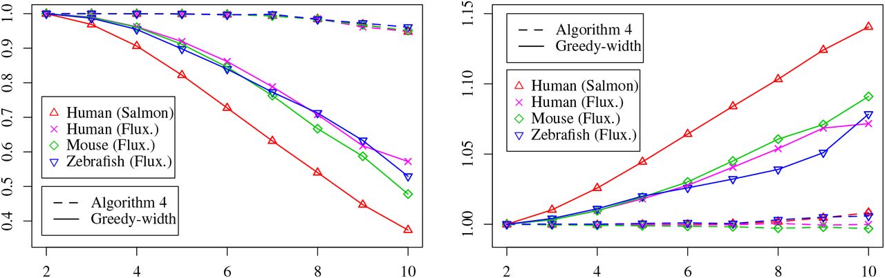
Based on |P‡|, for each dataset, we classify all instances into 10 categories, i.e., |P‡| ∈ {1, 2, …, 10}, and remove those instances with |P‡| > 10 (which is a tiny portion). For each category, we run both algorithms on all instances and compare their accuracy (proportion of instances that are predicted correctly), and average ratio between |P†| and |P‡| (i.e., mean value of |P†|/|P‡| over all instances).
The results are shown in Figure 8. We can observe that Algorithm 4 gives very high accuracy on all in-stances, while the accuracy of the greedy-width algorithm decreases rapidly as |P‡| increases. Meanwhile, the decompositions given by the greedy-width algorithm uses more paths and the ratio between the number of predicted paths and the ground truth keeps increasing as |P‡| increases, while for Algorithm 4 such ratio constantly remains closing to 1. These results demonstrate that in the application of transcript assembly, Algorithm 4 significantly outperforms the greedy-width algorithm.

Comparison of the two algorithm on transcript assembly. Left: x-axis is |P‡| and y-axis is the accuracy. Right: x-axis is |P‡| and y-axis is the average ratio between |P†|/|P‡|.
To evaluate the performance of our algorithm on large graphs, we carry out another set of experiments using simulated random instances. The results show that our algorithm can give very high accuracy for a wide spectrum of parameter combinations, while the greedy-width algorithm works well only for easy instances. These results further demonstrate the significant improvement of our algorithm over the greedy-width algorithm. The simulation setup and the detailed results are in Appendix B.
5 Discussion
We give an efficient heuristic for the minimum path flow decomposition problem. The components of this heuristic can be further improved. For example, we shall study how to reduce the optimality gap while keep optimality if a true nontrivial null vector is given, and also study how to identify nontrivial null vectors that are not simple as well as how to use such vectors to reduce the optimality gap. We tackle here only the flow decomposition step of transcript assebmly. Future work also includes extending our algorithm to develop a complete transcript assembler.
Acknowledgements
We thank Meiyue Shao and Guillaume Marc¸ais for helpful discussions and suggestions. This research is funded in part by the Gordon and Betty Moore Foundation’s Data-Driven Discovery Initiative through Grant GBMF4554 to Carl Kingsford, by the US National Science Foundation (CCF-1256087, CCF-1319998) and by the US National Institutes of Health (R21HG006913, R01HG007104). C.K. received support as an Alfred P. Sloan Research Fellow.
Appendix A Making Two Distant Edges Adjacent
In this Section, we describe an algorithm to make two given distant edges adjacent while keeping optimality. We first give some definitions to characterize the hierarchical structure of G. We say a pair of vertices (u, v) is connected (w.r.t. graph G), if there exists a path from u to v in G. For a pair of connected vertices (u, v), we define a subset V (u, v) ⊆ V as the set of vertices that are on some path from u to v (see Figure 5 (a,c)). Notice that if (u, v) is connected, we always have {u, v} ⊆ V (u, v). For a pair of connected vertices (u, v), we also define a subset E (u, v) ⊆ E as follows (see Figure 5): for any e ∈ E we say e ∈ E (u, v) if the both ends of e are in V (u, v). We say a pair of connected vertices (u, v) is closed, if for every vertex w ∈ V (u, v) \ {u, v}, all incident edges of w in E are also in E (u, v). We denote by  the set of all closed pairs. For each pair
  , we define Es(u, v) ⊆ E (u, v) as the set of edges in E (u, v) that are adjacent to u, and define Et (u, v) ⊆ E (u, v) as the set of edges in E (u, v) that are adjacent to v.
We define a reverse operation to modify G (Figure 5 (a,d)). For each pair  , we can reverse it by first detaching edges in Es(u, v) from u and attaching them to v, detaching edges in Et (u, v) from v and attaching them to u, and then switching the direction of all edges in E (u, v). Notice that we treat the reverse operation in a way that the set of edges in G is kept unchanged, but the locations and orientations of edges might be changed. Formally, let G′ be the graph after reversing
  . We assume that G′ still have the edge set of E. But for each edge ei = (u, v) in G, it might become ei = (u′, v′) in G′ with u′ ≠ u and/or v′ ≠ v. In other words, all edges are recognized by their original identities in E, and their adjacent two vertices might become different after performing reverse operations.
Let G′ be the graph after reversing  . Let (P′∗, w′∗) be one optimal decomposition of (G′, f). The following result states that solving Problem 1 on (G, f) is equivalent to solving it on (G′, f).
There exists a one-to-one correspondence between all decompositions of (G, f) and all decompositions of (G′, f). In particular, we have that |P∗| = |P′∗|.
Based on Proposition 12, we address the following problem.
Given two edges ei, ej ∈ E, decide whether we can perform a series of reverse operations, such that in the resulting graph we have ei = (u1, v1) and e j = (u2, v2) with either v1 = u2 or v2 = u1.
To solve Problem 3, we first describe a data structure to organize all the reverse operations. We define a binary relation  on
on  : for two pairs (u1, v1),
  , we say
  if V (u1, v1) ⊆ V (u2, v2). It is easy to verify that this relation forms a partial order. Let
  be the Hasse diagram on
  w.r.t. this partial order. For each edge in
  from (u1, v1) to (u2, v2), we remove it from
  if u1 ≠ u2 and v1 ≠ v2. We denote by
  this updated graph (see Figure 6).
We now describe an exact algorithm to solve Problem 3, which requires constructing  and then search-ing series of reverse operations guided by
  . We first compute the transitive closure of G, which gives us all possible connected pairs. For each connected pair (u, v), we follow the definition to check whether this pair is in
  : we compute V (u, v), which can be done in O(|V |) time with the availability of all connected pairs; then for each vertex w ∈ V (u, v) \ {u, v} we check whether all adjacent edges of w are still in V (u, v). It takes O(|E |) time to verify each connected pair, and thus the total running time to compute
  is O(|V |2 · |E |).
We then give an algorithm to compute  , i.e., for each pair in
  we need to compute its parents node in
  . For a subset V1 ⊆ V, |V1| ≥ 2, we say
  is a closure of V1, if we have V1 ⊆ V (u, v), and there does not exist
  such that V1 ⊆ V (u′, v′) ⊂ V (u, v). Intuitively, the closure of a given set of vertices is the smallest closed pair whose set of vertices contains the given vertices. As we will see in Proposition 13 such closure is unique. Now we describe an exact algorithm to compute the closure of a given subset, which shall be used in both constructing
  and the following steps (line 2 of Algorithm 6). The idea of this algorithm is to iteratively add necessary vertices until finally it becomes closed.
Exact algorithm to compute closure
Input: V1 ⊂ V,  and G
and G
Output: Closure of V1
1. Compute a topological ordering O of V, i.e., if (u, v) is connected, then O(u) < O(v).
2. Let S be the set containing all vertices in the final closure, initialized as V1.
3. Let L and R be the smallest and largest vertex in S according to their orderings in O, respectively.
4. Let Q be a queue that stores all (unexamined) vertices in S \ {L, R}, initialized as S \ {L, R}.
5. REPEAT
6. WHILE Q is not empty
7. Pop element v from Q.
8. FOREACH adjacent vertex u of v that is not in S
9. Insert u into S.
10. IF O(u) < O(L), push L to Q and set L = u.
11. IF O(u) > O(R), push R to Q and set R = u.
12. FOREACH adjacent vertex u of L that is not in S
13. IF  , insert u into S and push u to Q.
14. IF Q is empty, RETURN (L, R).
For any V1 ⊂ V, |V1| ≥ 2, Algorithm 5 returns the unique closure of V1 in O(|E |) time.
We now describe how to build  using Algorithm 5. Suppose that (u′, v′) is one of the direct parents of
  in
in  . We have two cases: either u ∉ {u′, v′}, or v ∉ {u′, v′}. If it is the first case, then (u′, v′) is exactly the closure of V1 = {u, v} ∪ {w | (w, u) ∈ E} ∪ {w | (u, w) ∈ E}. If it is the second case, then (u′, v′) is exactly the closure of V2 = {u, v} ∪ {w | (w, v) ∈ E} ∪ {w | (v, w) ∈ E}. In other words, the parents of
  in
in  are exactly the closures of V1 and V2. For each pair
  , we use this procedure to compute its parents, and thus the whole graph
  can be constructed. To further build
  , by definition, we then check each edge of
  to see whether the two pairs corresponding to its two adjacent vertices share the same starting or ending vertex. The total running time to build
  is O(|V |2 · |E |).
Exact algorithm for Problem 3
Input: G, ei = (u1, v1), ej = (u2, v2) ∈ E
Output: TRUE and series of reverse operations if they can be made adjacent, FALSE otherwise
1. Compute  .
.
2. Compute the closures of {u1, v1} and {u2, v2}; denote them as (u′1, v′1) and (u′2, v′2), respectively.
3. Initialize S1 = {u1}, T1 = {v1}, S2 = {u2}, T2 = {v2}.
4. Traverse  from (u′1, v′1): for each visited node
  , insert u to S1 and insert v to T1.
5. Traverse  from (u′2, v′2): for each visited node
  , insert u to S2 and insert v to T2.
6. IF S1 ∩ T2 = ∅ and S2 ∩ T1 = ∅, RETURN FALSE.
7. Compute arbitrarily w ∈ (S1 ∩ T2) ∪ (S2 ∩ T1); assume that w ∈ S2 ∩ T1.
8. Compute any path from (u′1, v′1) to node (·, w), and traverse this path to construct the reverse operations to make ei point to w: let (u, v) be the current node (i.e., ei is either points to v or leaves u) and u be the boundary vertex shared by (u, v) and its parent; reverse (u, v) if ei is not adjacent to u; move to the parent of (u, v) on this path. In the end reverse (·, w) if ei is not adjacent to w.
9. Perform the same procedure as line 8 to construct the reverse operations to make ej leave w.
10. RETURN TRUE.
Our complete algorithm to solve Problem 3 is described in Algorithm 6. The idea is first to locate the nodes in  for the given two edges, and then traverse
  starting from these two nodes respectively to compute all the possible positions that the two given edges can be moved to by reverse operations. After that the algorithm examines whether there exists a common vertex where the two edges can be made adjacent. The series of reverse operations can be obtained through tracing back. The correctness and running time of Algorithm 6 is stated as Proposition 14.
Algorithm 6 gives an exact solution for Problem 3 in O(|V |2 · |E |) time.
Appendix B Experiments with Simulated Random Instances
The simulation procedure first generates the ground truth (P‡, w‡), and then builds (G, f) based on them. In the simulation, we assume that G = (V, E) contains 1000 vertices, i.e., |V | = 1000, and assume that (1, 2, …, |V |) is one topological sorting of G. To generate a path p‡ in the ground truth, we first fix the length of this path, which is sampled uniformly at random from {1, 2, …, L}, where L ≤ |V | − 1 is a parameter governing the maximum length of the paths in the ground truth path. We then sample (|p‡| + 1) vertices uniformly at random without replacement from {1, 2, …, |V |}, and the path connects these vertices in an ascending order. The ground truth weight of this path, i.e., w‡(p‡), is sampled uniformly at random from {1, 2, …, 10000}. We repeat this process to generate |P‡| paths, where |P‡| is another parameter governing the number of paths in the ground truth. With (P‡, w‡), we then construct instance (G, f) by superposition of the weights of the paths that go through the edge (similar to Figure 7). Again, we denote by (P†, w†) be the output of the algorithm (Algorithm 4 or greedy-width), and we say (P†, w†) is correct if we have |P†| ≤ |P‡|.
We perform experiments with two different parameter settings, one is L = 50, |P‡| ∈ {20, 40, …, 200}, the other is L ∈ {10, 20, …, 100}, |P‡| = 100. For each parameter combination (L, |P‡|), we randomly generate 100 instances using the procedure mentioned above. We run both algorithms on these 100 instances, and for each algorithm we record its accuracy (proportion of instances that are predicted correctly), average ratio between |P†| and |P‡| (i.e., mean value of |P†|/|P‡| over the 100 instances), and total running time.
The results for the first parameter settings are shown in Table 1. First, we can observe that Algorithm 4 gives 100% accuracy when |P‡| ≤ 140, and it decreases a few percentage for larger |P‡|. Meanwhile, the accuracy of the greedy-width algorithm decreases rapidly with the increase of |P‡|, and drops to 0 when |P‡| ≥ 100. Second, we can see that the number of paths returned by Algorithm 4 is very close to the ground truth for all instances, while greedy-width algorithm uses more paths than the ground truth especially for large |P‡|. Third, both algorithms can finish these instances in a short amount of time, and Algorithm 4 is about 4 times slower than the greedy-width algorithm.
Comparison of the two algorithms on simulations with L = 50.
The results for the second parameter settings are shown in Table 2, which are consistent with that in Table 1. Combining these results we can conclude that Algorithm 4 can give decompositions with the same number of paths as that in the ground truth for a large scope of parameter combinations, while greedy-width algorithm can only give such decompositions for small L and small |P‡|, and it requires a significant portion of more paths for large L or large |P‡|. This shows a considerable improvement of Algorithm 4 over the greedy-width algorithm, especially for instances with many paths.
Comparison of the two algorithms on simulations with |P‡| = 100.
Appendix C Proofs of Propositions
Because (P∗, w∗) forms a decomposition of (G, f), we know that f = w∗ · P∗. By definition, for any  we also have P∗ · q = 0. Thus, we have that f · q = w∗ · P∗ · q = 0.
We can write Pr(f · q = 0) = Pr(w∗ · P∗ · q = 0). Since  , we know that P∗ · q ≠ 0. Combining the fact that elements in w∗ are sampled independently and uniformly at random from ℤk, using the standard backward analysis, we can conclude that Pr(f · q = 0) ≤ 1/k.
We can easily verify that for every row pi of  and for every v ∈ V0 we have that pi · qv = 0. Particularly, since
  , we have that P∗ · qv = 0. This implies that
  , for every v ∈ V0. Hence, we have
  .
.
According to the rank-nullity theorem, we have that  rank(P∗). From [24], we have that rows in the optimal solution are linearly independent, i.e., rank(P∗) = |P∗|. Besides, we also have that
  , since all vectors in {qv | v ∈ V0} are linearly independent. Combining all these facts, we have that
  .
.
We first prove that Algorithm 1 returns a subset of  . Let E1 ⊆ E and E2 ⊆ E be the two balanced subsets through tracing back from x ∈ D. We only need to show that E1 and E2 are indivisible. We first prove that E1 and E2 are disjoint. Suppose conversely that e ∈ E1 ∩ E2. Then we have B[|E |, x − f (e)] = 1, since there exist two subsets, namely E1′ = E1 \ {e} and E2′ = E2 \ {e}, such that f (E1′) = f (E2′) = x − f (e), a contradiction to the fact that x ∈ D.
Now we show that E1 and E2 are indivisible. Suppose conversely that there exist strict subsets E1′ ⊂ E1 and E2′ ⊂ E2 such that f (E1′) = f (E2′) = y. Let ek be the edge with the highest index in E1 ∪ E2. Without loss of generality, we assume that ek ∈ E1 \ E1′. Let ek′ be the edge with the highest index in E1′ ∪ E2′. We have that B[k′, y] = 1, because of the existence of E1′ and E2′. Following the recursion of B (line 4 of Algorithm 1), we also have that B[ j, y + ∑k′<i≤ j f (ei)] = 1, for all k′ < j ≤ k. This implies that B[k, x − f (ek)] = 1, a contradiction to the fact that x ∈ D.
We can verify that computing A, B, D and tracing back for all elements from D takes O(|E | · | f |) time, while other steps take less than that. Thus, the total running time of Algorithm 1 is O(|E | · | f |).
On one side, if there exists V1 ⊆ V0 such that  , then by definition, we have that
  .
.
Now we prove the other side. Assume that  , i.e.,
  . Let V1 = {v ∈ V0 | cv ≠ 0}. Let G1 = (V1, E1) be the subgraph of G induced by V1, i.e., we define e ∈ E1 if both ends of e is in V1. We first prove that G1 is weakly connected. Suppose conversely that G1 contains k ≥ 2 connected components,
  . We can write q = ∑1≤i≤k qi, where
  . Notice that qi contributes to distinct elements of q, i.e., for any edge
  , we have q[ j] = qi[ j]. Since
  , we also have that
  . Further, we have that
  , since we have
  . This implies that the two balanced subsets corresponding to q can be split into k pairs of balanced subsets, namely, Es(qi) and Et (qi), 1 ≤ i ≤ k, a contradiction to the fact that
  .
.
We now show that cv ∈ ℤ, ∀v ∈ V1. Let Es(V1) = {(u, v) ∈ E | u ∈ V \V1, v ∈ V1}, and Et (V1) = {(u, v) ∈ E | u ∈ V1, v ∈ V \V1}, Let Est (V1) = Es(V1) ∪ Et (V1). Let V2 ⊆ V1 be the subset of vertices that are adjacent to some edge in Est. For any edge ej = (u, v) ∈ E1, we have q[ j] = cv − cu. Following this formular, we have that cv ∈ {−1, +1}, ∀v ∈ V2, since edges in Est are adjacent to only one vertex in V1, which is in V2. Since G′ is weakly connected and q[ j] ∈ {−1, 0, +1}, by propagating from V2 with the above formular, we can conclude that cv ∈ ℤ for all v ∈ V1.
Consider any edge ej = (u, v) ∈ E1. If we assume that cu ≥ 1, then from the above formular we have that cv = cu + q[ j] ≥ 0; and since cv ≠ 0 and cv ∈ ℤ, we have that cv ≥ 1. Following this reasoning and the fact that G′ is weakly connected, through propagating we know that {cv | v ∈ V1} have the same sign. Without loss of generality, we assume that cv ≥ 1, ∀v ∈ V1. This implies that cv = 1, ∀v ∈ V2, and further implies that q[ j] = 1 for ej ∈ Es(V1) and q[ j] = −1 for ej ∈ Et (V1). Thus, we have that Es(V1) ⊆ Es(q) and Et (V1) ⊆ Et (q). According to flow conservation, we have that f (Es(V1)) = f (Et (V1)). Combining these two facts and the assumption that q is indivisible, we must have that Es(V1) = Es(q) and Et (V1) = Et (q). This consequently implies that V1 = V2. As we already have showed, cv = 1, ∀v ∈ V2, we have that  .
.
Suppose that  . According to Proposition 6, without loss of generality, we have that there exists a connected subset V1 ⊆ V0 such that
  . It is clear that q[ j] = 1 if and only if ej ∈ Es(V1), and q[ j] = −1 if and only if ej ∈ Et (V1), since for any edge ek that are adjacent to two vertices in V1 we have q[k] = 0. This yields that Es(q) = Es(V1) and Et (q) = Et (V1).
On the other side, suppose that there exists a subset V1 ⊆ V0 such that Es(q) = Es(V1) and Et (q) = Et (V1). We now prove that  . In fact,
  exactly has value of +1 for edges in Es(V1) = Es(q), and has value of −1 for edges in Et (V1) = Et (q). This yields that
  .
.
According to the algorithm, we can easily verify that  , from the fact that
  . We now show that
  . Suppose conversely that qk is not indivisible, i.e., there exist strict subsets E1 ⊂ Es(qk) and E2 ⊂ Et (qk) such that fk (E1) = fk (E2). Let ei ∈ Es(qk−1) and ej ∈ Et (qk−1) be the two chosen edges in iteration k. Assume that fk−1(ei) ≤ f k−1(ej). This implies that ei ∉ Es(qk). Let E1′ = E1 ∪ {ei}. If we further have f k−1(ei) = fk−1(ej), we define E2′ = E2 ∪ {ej}, otherwise, we define E2′ = E2. Clearly, we have that fk−1(E1′) = f k−1(E2′) according to the algorithm, and that E1′ and E2′ are strict subsets of Es(qk−1) and Et (qk −1), respectively, following from the fact that E1 and E2 are strict subsets of Es(qk) and Et (qk), respectively. Thus, we conclude that qk−1 is not indivisible, a contradiction.
We then show that  . Suppose conversely that
  . According to Proposition 6, there exists V1 ⊆ V0 such that Es(qk) = Es(V1) and Et (qk) = Et (V1). Let ei ∈ Es(qk−1) and ej ∈ Et (qk−1) be the two chosen edges in iteration k. Since
  , we know that either ei ∈ Es(V1) and ej ∈ Et (V1), or ei ∉Es(V1) and ej ∉ Et (V1). We further show the second case is not possible, since it immediately implies that qk−1 is not indivisible. Thus, we have that ei ∈ Es(V1) and ej ∈ Et (V1). If qk is obtained from the first situation (line 3) of Algorithm 3, then this already means that
  . Otherwise (line 6), since we guarantee that the path p used in line 8 of Algorithm 3 does not contain any edge in Es(qk−1) ∪ Et (qk−1), we can still conclude that
  , a contradiction, as desired.
Since qk is indivisible from Proposition 8, we know that during the k-th iteration, the two chosen edges ei and ej cannot have that f (ei) = f (ej), 1 ≤ k ≤ n − 1. According to Algorithm 3, we have that |Es(qk)| + |Et (qk)| = |Es(qk−1)| + |Et (qk−1)| − 1. After (n − 1) iterations, we must have that |Es(qk−1)| = |Et (qk−1)| = 1, and both the two subsets become empty after the n-th iteration. Thus, after exactly (|Es(q)| + |Et (q)| − 1) iterations, Algorithm 3 terminates.
We first prove that, for 1 ≤ k ≤ n − 1, we have that Δk ≤ Δk-1 Consider the change of number of edges and vertices during the k-th iteration. Let ei and ej be the two chosen edges. According to the proof of Proposition 9, we have that only ei will be removed, and a new edge (namely, ek in Algorithm 3) will be added. If it is the first situation (line 3 of Algorithm 3), then the middle vertex (namely, v1 = u2) cannot become isolated, since otherwise it implies that qk−1 is not indivisible. If it is the second situation (line 6 of Algorithm 3), some vertices in path p might be become isolated. But if this happens, then at least the same number of edges will also be removed in p. Thus, we always have that Δk ≤ Δk−1.
We now show that Δn ≤ Δn−1. This is because, in the n-th iteration, both ei and ej are removed, and only one edge will be added. Similar to the above analysis, if some vertices become isolated, then at least the same number of additional edges will be removed. Thus, we have that Δn ≤ Δn−1 − 1.
According to our analysis in the main text, the merging process narrows down the solution space, i.e., we have |Pk∗| ≥ |P(k−1)∗|, 1 ≤ k ≤ n. By combining these facts, we have that Δn − |Pn*| ≤ Δ − |P*| − 1.
The running time of Algorithm 4 is dominated by lines 2 and 3. According to Proposition 9, in Algorithm 3, Algorithm 6 will be called at most |E | times. Thus, according to Proposition 14 and the fact that  , the total running time is O(|V |2 · |E |2 · | f |).
Let (P, w) be any decomposition of (G, f). We can obtain a decomposition (P′, w′) of (G′, f) satisfying that |P′| = |P| and that w′ = w by only reversing the edges from u to v for each path in P. Since reverse operation is invertible, given a decomposition (P′, w′) of (G′, f), we can also obtain a decomposition (P, w) of (G, f) in the same way. This gives a one-to-one correspondence between the decompositions of (G, f) and that of (G′, f). And, in particular we have |P′∗| = |P∗|.
The correctness of the algorithm is the consequence of the following facts. First, if  , then among the vertices in V (u, v), u and v are the smallest and the largest vertices w.r.t. any topological ordering. This is simply because all vertices in V (u, v) \ {u, v} can be reached from u and can reach v. Second, L and R always store the current smallest and largest vertices in S w.r.t. the topological ordering. Thus, by definition, vertices added to S in line 9 of Algorithm 5 are guaranteed in the closure of V1. Third, Q always stores the vertices in S \ {L, R}. Thus, following the first fact, we know that vertices in Q cannot be the boundary vertices of the closure, and consequently, all their adjacent vertices (added in line 9) are guaranteed in the closure of V1. Fourth, when the algorithm terminates (line 14), we have that S= V (L, R). In fact, let p be any path from L to R. From line 13, we know that the first vertex in p is in S. Then following lines 8 to 11, all vertices in p will be added to S. Finally, all vertices in S \ {L, R} are examined such that all their adjacent vertices are in S. Thus, by definition, we know that (L, R) is closed. Besides, since all vertices added to S are guaranteed to in the closure of V1, we have that S is also the smallest subset, implying that (L, R) is the closure of V1. This reason also proves that the closure of V1 is unique. This algorithm is essentially the breadth-first search algorithm, in which edge each is examined at most once. Thus, its running time is O(|E |).
If Algorithm 6 finds w ∈ (S1 ∩ T2) ∪ (S2 ∩ T1), then clearly we can perform a series of operations to make ei and ej adjacent. On the other side, suppose that there exists a series of reverse operations such that in the resulting graph we have that ei = (w1, w) and ej = (w, w2). Let c1 and c2 be the closures of {w1, w} and {w, w2}, respectively. Clearly, all the reverse operations that moves ei (resp. ej) must operates on closures that are inside c1 (resp. c2). Thus, there must be a path from (u′1, v′1) (resp. (u′2, v′2)) to c1 (resp. c2) in  , which implies that Algorithm 6 will have w ∈ (S1 ∩ T2) ∪ (S2 ∩ T1). This reasoning also implies that when Algorithm 6 traces back to recover the reverse operations (lines 8 and 9), the two paths are disjoint, since they are in two different subtrees (rooted at c1 and c2, respectively).
The running time of Algorithm 6 is dominated by building  , which is O(|V |2 · |E |).


