

Abstract
The Developing Human Connectome Project (dHCP) seeks to create the first 4-dimensional connectome of early life. Understanding this connectome in detail may provide insights into normal as well as abnormal patterns of brain development. Following established best practices adopted by the WUMINN Human Connectome Project and pioneered by FreeSurfer, the project utilises cortical surface-based processing pipelines. In this paper, we propose a fully automated processingmechanisms, genetic pipeline for the structural Magnetic Resonance Imaging (MRI) of the developing neonatal brain. This proposed pipeline consists of a refined framework for cortical and sub-cortical volume segmentation, cortical surface extraction and cortical surface inflation of neonatal subjects, which has been specifically designed to address considerable differences between adult and neonatal brains, as imaged using MRI. Using the proposed pipeline our results demonstrate that images collected from 465 subjects ranging from 28 to 45 weeks post-menstrual age (PMA) can be fully automatically processed; generating cortical surface models that are topologically and anatomically correct. Downstream, these surfaces will enhance comparisons of functional and diffusion MRI datasets, and support the modelling of emerging patterns of brain connectivity.
1. Introduction
The period of rapid cortical expansion during fetal and early neonatal life is a crucial time over which the cortex transforms from a smooth sheet to a highly convoluted surface. During this time the cellular foundations of our advanced cognitive abilities are mapped out, as connections start to form between distant regions (Ball et al., 2013b; Van Essen, 1997), myelinating, and later pruning, at different rates. Alongside the development of this neural infrastructure, functional brain activations start to be resolved (Doria et al., 2010), reflecting the development of cognition.
Much of what is currently known about the early human connectome has been learnt from models of preterm growth (Ball et al., 2013b; Counsell et al., 2013; Doria et al., 2010; Keunen et al., 2017). Whilst invaluable, it is known that early exposure to the extra-uterine environment has long-term implications (Ball et al., 2012, 2013a; Counsell et al., 2014; Hintz et al., 2015; Ullman et al., 2015). For this reason the Developing Human Connectome Project (dHCP) seeks to image emerging brain connectivity, in a large cohort of fetal and term-born neonates, for the first time.
More broadly, the goals of the dHCP project are to pioneer advances in structural, diffusion and functional Magnetic Resonance Imaging (MRI), in order to collect high-quality imaging data for fetuses and (term and preterm) neonates, from both control and at-risk groups. Imaging sets will be supported by a database of clinical, behavioural, and genetic information, all made publicly available via an expandable, and user-friendly informatics structure. The dataset will allow the community to explore the neurobiological mechanisms, genetic and environmental influences, underpinning healthy cognitive development. Models of healthy development will provide a vital basis of comparison from which the effects of preterm birth, and neurological conditions such as cerebral palsy or autism, may become better understood.
The dHCP takes inspiration from the WU-MINN Human Connectome Project (HCP) (Van Essen et al., 2013). Now in its final stages, the HCP has pushed the boundaries of MRI based brain connectomics, collecting 1200 sets of healthy adult functional and structural connectomes, at high spatial and temporal resolution. Data from this project has been used to generate refined maps of adult cortical organisation (Glasser and Van Essen, 2011), and improve understanding of how the functional connectome correlates with behaviour (Smith et al., 2015)
A core tenet, underlying the success of the HCP approach, has been the advocation of surface-based processing and analysis of brain MR images. This is grounded in the understanding that distances between functionally specialised areas on the convoluted cortical sheet are more neurobiologically meaningful when represented on the 2D surface rather than in the 3D volume (Glasser et al., 2013). Surface-based processing therefore minimises the mixing of data from opposing sulcal banks or between tissue types. Further, surface-based registration approaches (Durrleman et al., 2009; Fischl et al., 1999c; Lombaert et al., 2013; Robinson et al., 2014; Wright et al., 2015; Yeo et al., 2010) improve the alignment of cortical folds and areal features.
Unfortunately, modelling cortical connectome structure in neonates and fetuses, is particularly challenging. Magnetic Resonance Imaging, and especially functional and diffusion protocols, are highly sensitive to head motion during scanning. This is a particular issue for the dHCP, where the goal is to image un-sedated neonatal, and free-moving fetal subjects. Therefore, correcting for this has required the development of advanced scanning protocols and motion correction schemes (Cordero-Grande et al., 2016; Hughes et al., 2016; Kuklisova-Murgasova et al., 2012).
Outside of the challenges facing acquisition and reconstruction the properties of neonatal and fetal MRI differ significantly from that of adult data. Specifically, baby and adult brains differ vastly in terms of size, with the fetal and neonatal brain covering a volume in the range of 100-600 millilitres in contrast to an average adult brain volume of more than 1 litre (Allen et al., 2002; Orasanu et al., 2014; Makropoulos et al., 2016). Furthemore, the perinatal brain develops rapidly and this results in vast changes in scale and appearance of the brain scanned at different weeks. This, together with the fact that scanning times must be limited for the well-being and comfort of mother and baby, means that spatial, and temporal resolution of the resulting images are reduced relative to adults. Furthermore, immature myelination of the white matter in neonatal and fetal brains results in inversion of MRI contrast relative to adults (Prastawa et al., 2005). This requires image processing to be performed on T2-weighted rather then T1-weighted structural MRI.
Combined, these vast differences in image properties, considerably limit the translation of conventional adult methods for image processing to fetal and neonatal cohorts. In particular, the popular FreeSurfer (Fischl, 2012) framework, utilised within the HCP pipelines (Glasser et al., 2013), fails on neonatal data as it relies solely on fitting surfaces to intensity-based tissue segmentation masks (Dale et al., 1999). These pipelines have been optimised to work with adult MRI data, and are not compatible with neonatal image distributions which are significantly different and vary drastically within different weeks of development. For this reason, simple adoption of the adult HCP processing pipelines has not been possible.
Instead, this paper presents a refined surface extraction and inflation pipeline, that will accompany the first data and software release of the dHCP project. This proposed framework builds upon a legacy of advances in neonatal image processing. This includes the development of specialised tools for tissue segmentation that address the difficulties in resolving tissue boundaries blurred through the presence of low resolution and partial volume. A variety of techniques have been proposed for tissue segmentation of the neonatal brain in recent years: unsupervised techniques (Gui et al., 2012), atlas fusion techniques (Weisenfeld and Warfield, 2009; Gousias et al., 2013; Kim et al., 2015), parametric techniques (Prastawa et al., 2005; Xue et al., 2007; Shi et al., 2010; Cardoso et al., 2013; Makropoulos et al., 2012; Wang et al., 2012; Wu and Avants, 2012; Beare et al., 2016; Liu et al., 2016), classification techniques (Anbeek et al., 2008; Srhoj-Egekher et al., 2012; Chiţă et al., 2013; Wang et al., 2015; Sanroma et al., 2016; Moeskops et al., 2016) and deformable models (Wang et al., 2011). A review of neonatal segmentation methods can be found in Devi et al. (2015); Makropoulos et al. (2017). The majority of these techniques have been applied on lower resolution images to the ones acquired within the dHCP project and typically on preterm subjects.
Once segmentations are extracted, surface mesh modelling approaches are, to an extent, agnostic of the origin of the data; allowing, in principle, the application of a wide variety of cortical mesh modelling approaches, to neonatal data, including those provided within the FreeSurfer (Dale et al., 1999; Fischl, 2012), Brainsuite (Shattuck and Leahy, 2002) and Brainvisa (Rivière et al., 2009) packages. In general, these methods fit surfaces to boundaries of tissue segmentation masks which, allowing for some need for topological correction, relies on the accuracy of the segmentation. In neonatal imaging data, however, the use of T2 images, leads to segmentation errors not seen in adult data. This is the misclassification of CSF as white matter, caused by the fact that CSF and white matter appear bright in neonatal T2 images, whereas in adult T1 data white matter is bright and CSF is dark. If not fully accounted for during segmentation, these errors will be propagated through to surface reconstruction (Xue et al., 2007).
In what follows we present a summary of our proposed pipeline. This brings together existing tools for neonatal segmentation (refined to minimise the propagation of misclassification errors through to surface extraction) with new tools for cortical extraction that combine information from segmentation masks, and T2-weighted image intensities in order to generate topologically and anatomically correct surfaces. Re-implementations of existing tools for surface inflation and projection to the sphere are provided to minimise software overhead for users.
The processing steps are as follows: 1) acquisition and reconstruction of T1 and T2 images (Cordero-Grande et al., 2016; Hughes et al., 2016; Kuklisova-Murgasova et al., 2012); 2) tissue segmentation and regional labeling (Makropoulos et al., 2012, 2014a, 2016); 3) cortical white and pial surface extraction (Schuh et al., 2017); 4) inflation and projection to a sphere (for use with spherical alignment approaches) (Fischl et al., 1999a; Elad et al., 2005); and 5) definition of cortical feature descriptors, including descriptors of cortical geometry and myelination (Glasser et al., 2013). Manual quality control is performed by two independent expert raters to assess the quality of the acquired images, segmentations and reconstructed cortical surfaces. Assessment of these data sets shows that, with very few exceptions (3%), the protocol is able to extract cortical surfaces that fit closely with expectations for observed anatomy.
2. Project Overview
The goal of the Developing Human Connectome Project is to create a dynamic map of human brain connectivity from 20 to 45 weeks postconceptional age from healthy, term-born neonates, infants born preterm (prior to 36 weeks PMA), and fetuses. The infants are being scanned using optimised protocols for structural (T1 and T2-weighted) images, resting state functional Magnetic Resonance Imaging (fMRI), and multi-shell High Angular Resolution Diffusion Imaging (HARDI). Imaging data will be combined with genetic, cognitive and environmental information in order to aid understanding of the developing human brain and give crucial insight into brain vulnerability and disease development. Novel image analysis and modeling tools will be developed and integrated into HCP inspired surface-processing pipelines in order to extract structural and functional connectivity maps. All data, and supporting software will be made publically available within an expandable, future-proof informatics structure that will provide the research community with a user-friendly environment for hypothesis-based studies and allow continual ongoing addition of new data.
3. The Neonatal Structural Pipeline
The first stage of the project has been to optimise acquisition protocols and collect data for the neonatal cohort (Cordero-Grande et al., 2016; Hughes et al., 2016; Kuklisova-Murgasova et al., 2012). The methods in this paper therefore reflect neonatal structural processing protocols, and are designed to accompany the first data release of neonatal subjects.
The workflow of the neonatal processing pipeline is summarised in Fig. 1. First motion-corrected, reconstructed T1 and T2-weighted (T1w and T2w) images are bias-corrected (the T2 image is further brain-extracted). Then, the T1 image is aligned with the T2 image using rigid registration (A) and brain-extracted with the mask calculated from the T2 image. Following this, the T2 MRI is segmented into different tissue types (cerebrospinal fluid, CSF, white matter, WM, cortical grey matter, cGM, and subcortical, GM) using the Draw-EM algorithm (based on Makropoulos et al. (2014b) section 3.2) (B). Next, white matter masks are split along the mid-line between the hemispheres and filled to represent binary masks for each hemisphere, and topologically correct white matter surfaces are fit to the grey-white tissue boundary (section 3.3)(C). Pial surfaces are then generated by expanding each white matter mesh towards the grey-CSF tissue boundary (D), and mid-thickness surfaces are generated halfway between the pial and the white, by taking the Euclidean mean of the vertex coordinates (E). The cortical thickness is also estimated based on the Euclidean distance between the white and pial surface. In a separate process, inflated surfaces are generated through expansion-based smoothing of the white surface (F). This acts as initialisation to a Multi-Dimensional Scaling (MDS, section 3.4) scheme that projects all points onto a sphere, whilst preserving relative distances between neighbouring points. Finally, surface geometry and myelo-structure are summarised through a series of surface feature maps. These include: G) maps of mean surface curvature, estimated from the white surface; H) maps of mean convexity/concavity (sulcal depth); estimated during inflation; and I) maps of cortical myelination; estimated from the ratio of T1w and T2w images projected onto the surface.

Structural pipeline steps: A) Pre-processing; B) Tissue segmentation (shown as contour map); C) White-matter mesh extraction; D) Expansion of white surface to fit the pial surface; E) Fitting of mid-thickness surface mid-way between white and pial and estimation of thickness; F) Inflation of white surface to fit the inflated surface and projection onto a sphere; G) Estimation of surface curvature from the white surface; H) Estimation of sulcal depth maps (mean convexity/concavity); I) Estimation of T1/T2 myelin maps;
Following adult frameworks, proposed for FreeSurfer (Fischl et al., 1999b), and refined by the Human Connectome Project (Glasser et al., 2013), all computed surfaces of each subject (white, pial, mid-thickness, inflated, spherical) have one-to-one point correspondence between vertices. This ensures that, for each individual brain the same vertex index represents the same relative point on the anatomy for all these surfaces. In other words, two corresponding points on the white and pial surface would approximate the endpoints of where a column of neurons through the cortex would travel. This simplifies downstream processing, and facilitates straightforward visualisation of features across multiple surface views.
3.1. Acquisition
The data used in the paper were collected at St. Thomas Hospital, London, on a Philips 3T scanner using a 32 channel dedicated neonatal head coil (Hughes et al., 2016). To reduce the effects of motion, T2 images were obtained using a Turbo Spin Echo (TSE) sequence, acquired in two stacks of 2D slices (in sagittal and axial planes), using parameters: TR=12s, TE=156ms, SENSE factor 2.11 (axial) and 2.58 (sagittal) with overlapping slices (resolution (mm) 0.8×0.8 × 1.6). Motion corrected reconstruction techniques were employed combining Cordero-Grande et al. (2016); Kuklisova-Murgasova et al. (2012) resulting in isotropic volumes of resolution 8×0.8×0.8mm3. T1 images were acquired using an IR (Inversion Recovery) TSE sequence with the same resolution with TR=4.8s, TE=8.7ms, SENSE factor 2.26 (axial) and 2.66 (sagittal). Subjects were not sedated, but imaged during natural sleep. All images were reviewed by an expert paediatric neuroradiologist and checked for possible abnormalities. In this paper we report results from 453 subjects that have been processed through the proposed pipeline. 38 subjects had repeat longitudinal scans resulting in a total 492 scans. The distribution of ages at birth and ages at scan is shown in Fig. 2.

Distribution of age at birth and age at scan for the 453 processed subjects (492 scans).
3.2. Segmentation
The T2w image data is segmented into 9 tissue classes (Table 1), using the Draw-EM 2 (Developing brain Region Annotation With Expectation-Maximization) algorithm. This is an open-source software for neonatal brain MRI segmentation based on the method proposed in Makropoulos et al. (2014a).
Tissue labels.
Regional labels segmented with Draw-EM (based on the atlases of (Gousias et al., 2012)). These total 87 regions (note cortical regions are further spilt into cortical/subcortical components).
In summary, segmentation proceeds following brain-extraction, implemented using the Brain Extraction Tool (BET) (Smith, 2002), in order to remove non-brain tissue. Then images are corrected for intensity inhomogeneity with the N4 algorithm (Tustison et al., 2010). Segmentation is performed with an Expectation-Maximization (EM) algorithm that includes a spatial prior term and an intensity model of the image, similar to the approach described in Van Leemput et al. (1999). The spatial prior probability of the different brain structures is defined based on multiple labelled atlases manually annotated by Gousias et al. (2012) 3. These atlases are registered to the target image, and their labels are transformed and averaged according to the local similarity of each atlas (based on the local Mean Square Distance as proposed in Artaechevarria et al. (2009). The intensity model of the image is approximated with a Gaussian Mixture Model (GMM). Spatial dependencies between the brain structures are modelled with Markov Random Field (MRF) regularisation. The segmentation algorithm further includes CSF-WM partial volume correction to correct for the similar intensity of CSF to the WM along the CSF-cGM boundary, and model averaging of EM and label fusion to limit the influence of intensity in the delineation of structures with very similar intensity profiles. The resulting segmentation contains 87 regional structures (see Table 1). These are merged to further produce the following files: tissue labels, left/right white surface masks and left/right pial surface masks.
The dHCP data differs significantly from previous neonatal cohorts collected by this consortium, in that the vast majority of the data in previous studies were acquired from prematurily-born neonates and typically at lower spatial resolutions. Thus Draw-EM includes several modifications with respect to Makropoulos et al. (2014a) in order to maximise the benefits for downstream processing. These include: modelling of additional tissue classes to account for the presence of hyper/hypo intense pockets of white matter, which occur naturally in the maturing brain; together with improvements afforded by a multi-channel volumetric registration, which simultaneously registers both subjects’ T2 images and their grey-matter tissue segmentation masks (obtained from a preliminary run of the segmentation algorithm - see below).
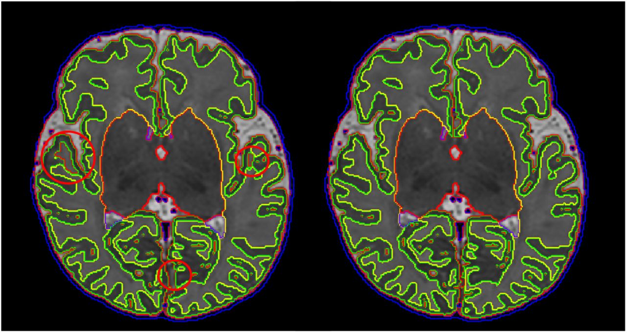
All major steps of the Draw-EM pipeline are summarised in Fig. 6. An example segmentation using Draw-EM is illustrated in Fig. 7. The importance of the modifications to the segmentation approach are demonstrated through Figures 3 to 5. Specifically, Fig. 3 demonstrates improvements to segmentation accuracy through modelling two additional tissue classes: 1) low and 2) high intensity WM. Here, the low-intensity WM class is included to account for myelinated WM that is often mislabelled for cGM in particular around the insula and the frontal lobe, and the high-intensity WM class is included to correct for WM hyper-intensities around the ventricular area that are often mislabelled as ventricles. Low-intensity and high-intensity WM classes are merged to WM after the segmentation has completed.

a) Segmentation of a subject T2 without and with the inclusion of the low-intensity WM class (left and right image respectively). b) Segmentation of a subject T2 without and with the inclusion of the high-intensity WM class (left and right image respectively). Affected areas are noted with a red circle.
The labelled atlases (Gousias et al., 2012) are registered to the subject using a multi-channel registration approach, where the different channels of the registration are the original intensity T2-weighted images and GM probability maps. These GM probability maps are derived from an initial tissue segmentation, performed using tissue priors propagated through registration of a preterm probabilistic tissue atlas Serag et al. (2012) to each term-born subject. Preterm subjects typically have increased CSF volume over term neonates (Makropoulos et al., 2016), and this is reflected in the preterm template Serag et al. (2012). Therefore, to account for the effects of misregistration resulting from the different amounts of CSF (see Fig. 4), we use a trimmed version of the pre-term template (eroding CSF intensities from the template image) to perform the registration and initial tissue segmentation. Afterwards, these initial GM maps are then used along with the intensity T2-weighted images in the multi-channel registration of the labelled atlases (Gousias et al., 2012). Fig. 5 presents the benefit of using a multi-channel registration approach instead of a single-channel registration using only the intensity. It has been found that inclusion of the GM probability maps improves the accuracy of the alignment of the cortical ribbon, despite the large differences in cortical folding that are observed throughout the developing period. For more details on the individual parts of the original segmentation pipeline we refer the reader to Makropoulos et al. (2014a).

Segmentation of a subject T2 based on the original preterm template Serag et al. (2012) and the trimmed template registration (right image). Affected areas are noted with a red circle.
Segmentation of a subject T2 with single-channel registration (left image) and multi-channel registration (right image). Affected areas are noted with a red circle.
3.3. White, Pial and Mid-thickness Surface Extraction
Following segmentation, white-matter mesh extraction is performed by fitting of a closed, genus-0, triangulated surface mesh (convex hull) onto the inferred white-matter segmentation boundary. In order to regularise for the effects of partial volume, which can lead to incorrect assignment of CSF voxels to either white or cortical grey-matter tissue classes, we refine the shape of the mesh by incorporating intensity information from the bias-corrected T2 and (if available) T1 images (Schuh et al., 2017).
In Schuh et al. (2017), the deformation of the initial genus-0 surface, inwards towards the white-grey tissue boundary, is governed through a tradeoff between external and internal forces. Specifically, the external force seeks to minimise the distance between the placement of the surface mesh vertices and the locations of the tissue boundaries, and this is regularised by three different internal forces, which seek to: 1) enforce smoothness by reducing curvature; 2) flatten creases in the mesh along sulcal banks; and 3) discourage mesh intersections by introducing a repulsion force between adjacent nodes.
Surface reconstruction proceeds over two stages, where, in the first stage, external forces are derived from distances to the tissue segmentation mask, and in the second stage, boundaries are refined using external forces derived from intensity information: specifically, the force attracts each vertex node towards the closest WM/cGM edge in the normal direction.
The closest WM/cGM edge in the second stage is found by analyzing the one-dimensional intensity profile and directional derivative sampled at equally-spaced ray-points. Examples are shown in Fig. 8. Here, a white-matter boundary edge occurs between a maximum with WM intensity, followed by a minimum with cGM intensity (left/right of green vertical line). Starting at the ray center (red vertical line, yellow dot), a suitable edge is found by searching both inwards and outwards from the node until either a WM/cGM edge is found, a maximum search depth is exceeded, or the ray intersects the surface. Further examples of the improvements gained by intensity based refinement, over a straightforward fit to the segmentation boundary, are shown in Fig. 9. Finally, a median filtering and Laplacian smoothing of surface distances is performed to reduce the influence of small irregularities in the segmentation boundary. Small holes in the segmentation manifest themselves in the surface distance map as small clusters of supposedly distant points as seen left of Fig. 10. These are filled in to avoid the surface mesh to deform into them.

The major steps of the Draw-EM pipeline are: 1) Pre-processing. The original MRI is brain-extracted and corrected for intensity inhomogeneity; 2) The preterm atlas template is registered to the bias-corrected T2 image and an initial (tissue) segmentation is generated; 3) The GM probability map obtained from the initial segmentation is used together with the MR intensity image as different channels of a multi-channel registration of the labelled atlases by (Gousias et al., 2012) to the subject. 4) Regional labels are segmented based on the labels propagated from the atlases; 5) Segmented labels are merged in different granularities to further produce the following files: tissue labels, left/right White surface masks and left/right pial surface masks.

Example segmentation using Draw-EM. The subject T2, label segmentation, tissue segmentation, white surface and pial surface mask are presented from left to right.

Intensity (blue curve) and derivative (dashed curve) sampled at blue crosses. The yellow dot marks the mesh node on the initial surface (red). The green contour depicts the white-matter surface. Yellow arrows point at the cGM/CSF edge of the pial surface.

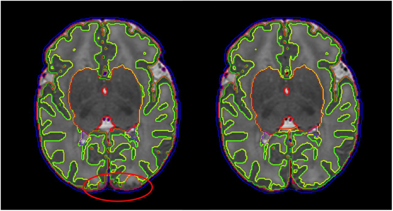
Segmented T2w image intersected by white and pial surfaces (left). White boxes outline corrections in areas where CSF appears dark due to partial volume effects, and yellow boxes corrections in areas where the CSF has been mislabelled as WM. Zoom of white surface mesh before (middle) and after (right) edge-based refinement. The top row demonstrates correction of a sulcus by moving the surface inwards, and the bottom row correction of a segmentation hole by moving the surface outwards.

WM segmentation boundary distance in normal direction, before clustering based hole filling (left), and after the hole filling and smoothing (right). A number of holes in the segmentation are indicated by yellow arrows.

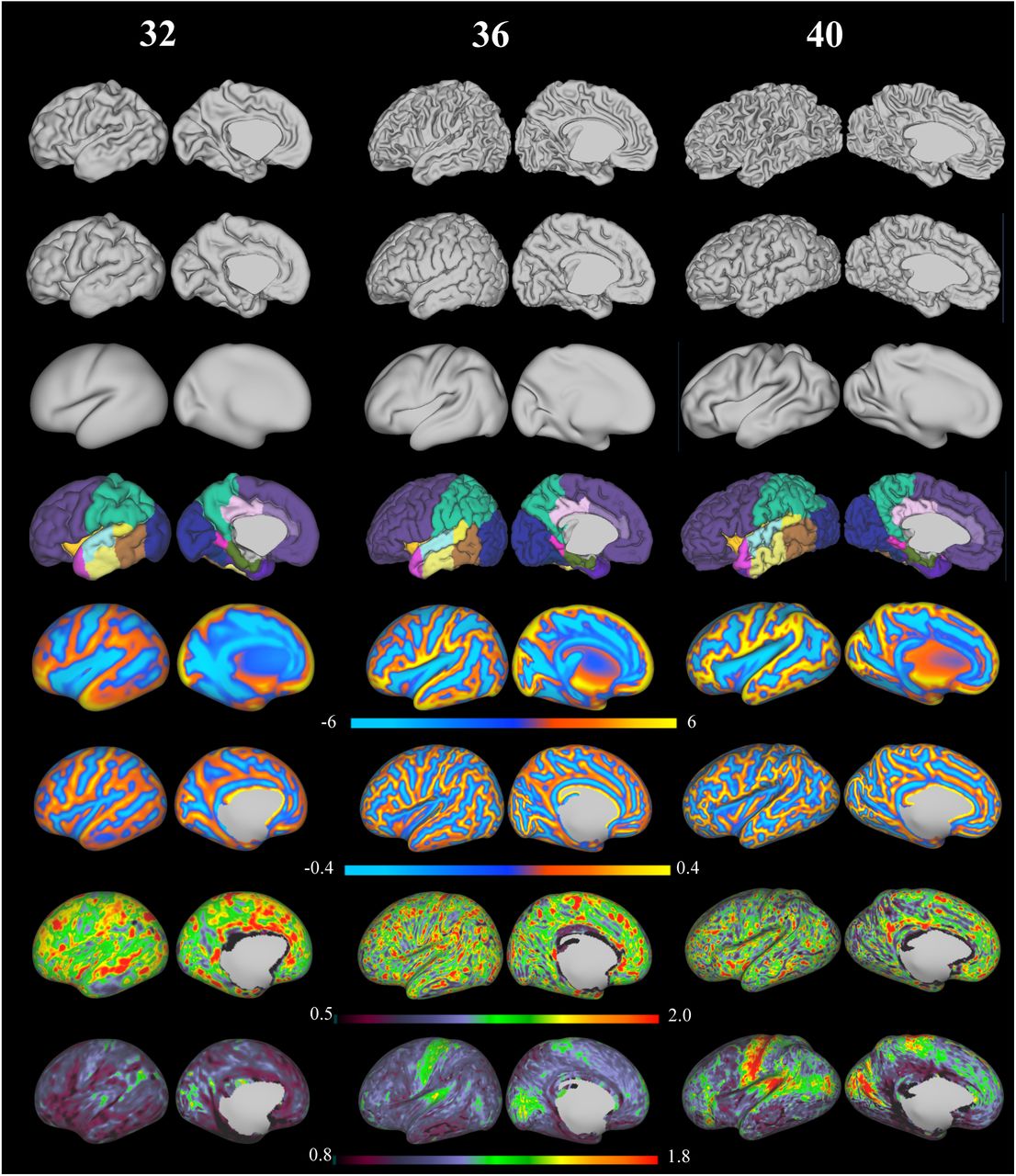
Exemplar surfaces and feature sets for three individuals scanned at 32, 36 and 40 weeks PMA (left hemisphere). From top to bottom: white surface, pial surface, inflated surface, cortical labels, sulcal depth maps, mean curvature, cortical thickness and T1/T2 myelin maps (all features shown on the very inflated surface)
Next, the pial surface is obtained by deforming the white-matter mesh towards the cGM/CSF boundary using the same model but modifying the external force to search for the closest cGM/CSF image edge outside the white-matter mesh. These edges correspond to a positive derivative in normal direction of the T2 intensity (yellow arrows in Fig. 8). When no such edge is found, e.g. within a narrow sulcus due to partial volume, the opposing sulcal banks expand towards each other until stopped by the non-self-intersection constraint. Finally, a mid-thickness surface is generated half-way in-between by averaging the positions of corresponding nodes. Please refer to Schuh et al. (2017) for more details on the surface reconstruction.
3.4. Surface Inflation and Spherical Projection
In a separate process, the white matter surface is inflated using a reimplementation of the inflatable surface model of FreeSurfer (Fischl et al., 1999a). This uses an inflation energy functional that consists of an inflation term, that forces the surface outwards (for vertex points in sulcal fundi) and inwards (for points on gyral crowns), and a metric-preservation term that preserves distances between neighbouring points. Surfaces are expanded until they fulfil a pre-set smoothness criterion (Fischl et al., 1999a).
As a by-product of the surface inflation, a measure of average concavity/convexity is obtained for each vertex. This represents the change of a node’s position in normal direction, and is proportional to the depth of major sulci.
In a final step, inflated meshes are projected onto a sphere using spherical Multi-Dimensional Scaling (MDS) as proposed by (Elad et al., 2005). This computes an embedding, or projection, of each inflated mesh onto a sphere, whilst minimising distortion between mesh edges. More specifically, the projected positions of vertex points on the sphere are optimised so as to preserve the relative distances between points, as measured in the initial inflated mesh space. In each case, the distances (measured for the sphere and the input mesh) are estimated as geodesics, and are computed using a fast marching method for triangulated domains (Kimmel and Sethian, 1998). Note, the input mesh must first be scaled so that its surface area is equal to that of the unit sphere.
3.5. Feature Extraction
The processes of surface extraction and inflation generate a number of well known feature descriptors for the geometry of the cortical surface. These include: surface curvature estimated from the mean curvature (or average of the principal curvatures) of the white matter surface; cortical thickness estimated as the Euclidean distance of corresponding vertices between the white and the pial surface; and sulcal depth which (as mentioned above) represents average convexity or concavity of cortical surface points estimated during the inflation process.
In addition to geometric features, the pipeline also estimates correlates of cortical myelination using the protocol described in Glasser and Van Essen (2011); adopted by the HCP. These feature maps are estimated from the ratio of T1-weighted and T2-weighted images and represent an architectonic marker that reliably traces areal boundaries of cortical areas and correlates with cytoarchitecture and functionally distinct areas in the cortex Glasser and Van Essen (2011). As the neonatal pipeline is based on T2w image processing rather than T1w (as for the adults), neonatal T1/T2 myelin maps are estimated by first rigidly registering each T1w image to its T2w image pair. Following this, the T1:T2 ratio is projected onto the mid-thickness surface, using volume-to-surface mapping (Glasser et al., 2013).
Further, regional labels (from the method described in Gousias et al. (2012)) are automatically generated during segmentation. These regional labels are further projected onto the cortical surface. The closest voxel in the volume with respect to each vertex in the mid-thickness surface is used to propagate the label to that vertex. The projected labels are consequently post-processed with filling of small holes and removal of small connected components.
Fig 11 depicts exemplar surfaces for three subjects aged 32, 36 and 40 weeks PMA (at time of scan) together with cortical labels, sulcal depth, cortical thickness, mean curvature, and T1/T2 myelin maps. This demonstrates the considerable differences in surface geometry and myelination over the developmental period covered by this cohort.
4. Quality Control (QC)
The quality of the pipeline was assessed by manually scoring a sub-set of randomly selected images from the cohort. We performed three independent scorings for the different parts of the pipeline: image reconstruction, segmentation and surface extraction. Note, 160 images were used during image and segmentation QC; a sub-set of 43 was then used for the more manually intensive surface QC. All images and surfaces were scored independently by two expert raters (one neuro-anatomist, one methods specialist) to assess inter-rater agreement. The image and segmentation QC was performed by AM and SJC and surface QC by AM and JS. The results are presented in the following sections.
4.1. Image QC
Quality checking of neonatal images was performed by first binning all subjects’ PMA (at scan) into weeks (in the range: 37-44 weeks) and selecting 20 images at random from each weekly interval. This yielded a total of 160 images. Note, the relatively low limit of 20 per week was selected due to the limited amount of images (57 out of the total 492 scans, less than 20 per age) acquired at earlier scan ages (29 - 36 weeks). The protocol for manual scoring of the image quality is presented in Fig. 12. Scoring was performed by visual inspection of the whole 3D volume slice by slice. Poor quality images were rated with score 1. Images with significant motion were rated with score 2. Images with negligible motion visible only in a few slices were rated with score 3. Images of good quality with no visible artifacts were rated with score 4.

Manual QC score of image quality. From left to right: poor image quality - score 1, significant motion - score 2, negligible motion - score 3, good quality image - score 4.
Fig. 13 presents the percentage of images rated with the different scores by the two reviewers. On average, 90% of the images were considered to have negligible or no motion (score 3 and 4) and only 2% of the images had to certainly be discarded due to poor image quality according to the raters. The raters’ scoring was the same in 78% of the images and within a difference of one scoring point in 99% of the images.

Image scores from the 2 raters (based on 160 images).
4.2. Segmentation QC
Following image QC, tissue segmentation masks were evaluated for the same set of subjects. Quality was assessed using the protocol presented in Fig. 14. Specifically, images that were poorly segmented were rated with score 1; images with regional errors were rated with score 2; images with localised segmentation errors were rated with score 3; images with segmentations of good quality with no visible errors were rated with score 4.

Manual QC score of segmentation quality. From left to right: poor segmentation quality - score 1, regional errors - score 2, localised errors - score 3, good quality segmentation - score 4.
Here, regional errors often occured at the interface between the cerebellum and the inferior part of the occipital and temporal lobe, where part of the cortical ribbon was mislabelled as cerebellum due to poor image contrast between the regions; another source of regional problems was when WM was mislabelled as cGM or CSF due to partial volume effects. By contrast, localised errors typically occurred when the CSF inside a sulcus was mislabelled as WM due to partial voluming effects. We further refer the reader to Makropoulos et al. (2014a) for additional validation of the segmentation method.
The scores attributed by the two raters are presented in Fig. 15. Poor segmentation occured only in 5 scans (3% of cases) and these were related to poor image quality or significant motion (image score 1 and 2). Regional (24% of cases) and localised errors (64% of cases) were present in the majority of the cases. The scoring of the raters agreed in 71% of the images and was within a difference of one scoring point in 99% of the images.
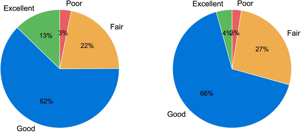
Segmentation scores from the 2 raters (based on 160 images).
Furthermore, we assessed the improvements with the proposed segmentation. We manually inspected segmentations of all the 492 scans obtained with: a) the proposed segmentation method and b) the tissue segmentation method outlined in Makropoulos et al. (2012), that uses the original template from Serag et al. (2012) for the atlas priors, as baseline (Makropoulos et al. (2012) presented the most accurate results in the NeoBrainS12 challenge (Išgum et al., 2015)). Fig. 16 presents the occurence of the different segmentation problems presented in Section 3.2 with the baseline and the proposed method: top part of cGM missing (see Fig. 4), CSF inside WM (see Fig. 5), hyper-intense WM misclassified as ventricles (see Fig. 3), hypo-intense WM misclassified as cGM (see Fig. 3). The segmentation method with the proposed modifications has diminished the occurences of this problems (top part of cGM missing in 1.6% compared to the baseline 23.8% of cases, CSF inside WM in 1.4% compared to 36.4%, hyper-intense WM misclassified as ventricles in 7.7% compared to 90.7% and hypo-intense WM misclassified as cGM in 0% compared to 84.6%). These problems, where still present in the proposed method, are typically reduced in extent.

Occurerence of segmentation problems with the baseline segmentation method (Makropoulos et al., 2012) and the proposed segmentation (based on 492 images).
4.3. Surface QC
Cortical surface quality was assessed by visual scoring of the reconstructed white surface. Visual surface QC by an expert was performed for a number of regions of interest (ROIs), automatically selected per subject. In order to specifically focus the surface QC on the improvements of the reconstructed surface over the tissue segmentation boundary produced from Draw-EM, we aimed to identify regions that deviate from this boundary. We additionally reconstructed each surface with an alternative surface extraction technique that faithfully follows the tissue mask segmentation boundaries (Wright et al., 2015). Surface QC then proceeded for ROIs where the surfaces extracted from the two techniques (Schuh et al. (2017) and Wright et al. (2015)) deviated most from each other. ROIs were viewed in image volume space as 3D patches (of size 50 × 50 × 50 mm) located at the center of each cluster, with the white surface shown as a contour map (see Fig. 17 for examples of the ROI visualization). Due to the large number of patches, a subset of 43 images was used from the 160 images included for the image and segmentation QC. 20 ROIs were selected for each subject and were rated independently. Scoring of the surfaces was done by assigning a score from 1 to 4 for each ROI according to the protocol in Fig. 17: score 1 was rated as poor quality (this happened typically in cases where the contour substantially deviated from the cortical boundary or there were extensive missing gyri); score 2 was assigned in cases where the contour was close to the cortical boundary but there were obvious mistakes; score 3 was used for contours that were accurate but contained some minor mistakes; score 4 indicated an accurate contour tracing of the cortical boundary.

Manual QC score of surface quality. From left to right: poor surface quality - score 1, contour close to the cortical boundary but with obvious mistakes - score 2, minor mistakes - score 3, good quality surface - score 4.
Fig. 18 presents the results of the surface QC. The proposed method produced surfaces that were rated as accurate (score 3 or 4) in 85% of the ROIs with 49% presenting no visual mistakes, averaged between the two raters. The remaining percentage of ROIs (15%) were rated as having obvious mistakes but being close to the cortical boundary (score 1 or 2), with only less than 2% having poor quality (score=1). The scoring of the raters was the same in 52% of the ROIs and was within a difference of one scoring point in 93% of the images. Fig. 19 demonstrates examples of improvements with the proposed method over a surface extracted to faithfully follow the segmentation boundary.

Scoring of surface ROIs from the 2 raters (based on 43 images with 20 ROIs per image).
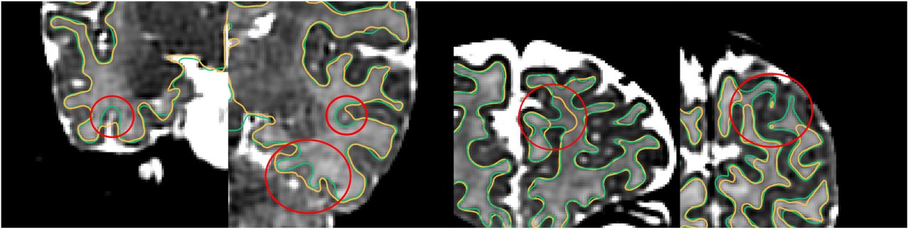
Comparison of surfaces produced with the proposed method (overlaid with green color) over surface extraction that follows the tissue segmentation boundary produced from Draw-EM (overlaid with yellow color).
5. Discussion
This paper presents a finalised pipeline for brain tissue segmentation and cortical surface modelling of neonatal MRI. All methods have been tuned on images collected using the dHCP protocol, and take advantage of improvements in image quality (gained from advances in acquisition, reconstruction and motion correction (Cordero-Grande et al., 2016; Hughes et al., 2016; Kuklisova-Murgasova et al., 2012)) to offer topologically correct and accurate surface representations for neonatal images, acquired between 28 and 45 weeks PMA.
The goal of the dHCP project is to develop the first four-dimensional model of emerging functional and structural brain-connectivity. Accordingly, the dHCP is pushing the boundaries of structural, functional and diffusion image acquisition, to improve the spatial resolution of T1 and T2-weighted images, the angular resolution of diffusion MRI (dMRI) and the temporal resolution of functional MRI (fMRI), relative to previous neonatal and fetal studies. The results in this paper represent the foundations of a surface-constrained set of functional and diffusion analysis pipelines, inspired by frameworks proposed by the HCP (Glasser et al., 2013; Van Essen et al., 2013), and based on FreeSurfer methods for surface extraction (Fischl et al., 1999b; Fischl, 2012). Studies have shown that surface-constrained analyses: improve the localisation of functional units along the cortical surface (Fischl et al., 2008; Glasser et al., 2013, 2016b; Van Essen et al., 2012); reduce the mixing of white and grey matter fMRI signals during smoothing (Glasser et al., 2013); and increase the alignment of functional areas during registration (Durrleman et al., 2009; Fischl et al., 1999c; Lombaert et al., 2013; Robinson et al., 2014; Wright et al., 2015; Yeo et al., 2010).
However, surface-constrained analyses rely on highly (geometrically) accurate reconstructions of the cortical surface. FreeSurfer-derived HCP pipelines do not work for neonates, whose brains are smaller and still developing. Neonatal images present inverted tissue intensity profiles, hypo/hyper intense white-matter patches and, due to the smaller size of the imaged structures, even for same image resolution, they are more prone to partial volume effects than for adult MRI. Further, dHCP neonates are imaged during natural sleep. As a result, motion artifacts are a concern, with a small subset of acquisitions heavily affected.
FreeSurfer (FS) methods for surface extraction depend on tissue segmentation models that are largely intensity-based (Dale et al., 1999). These are not robust to noise and are un-suited to the inverted tissue intensity distributions, and increased partial volume of neonatal data. Further, FreeSurfer white cortical surface mesh modelling approaches rely on tessellating topologically correct white matter tissue segmentations, and FS pial surface extraction tools require tissue intensity information; making implicit assumption that the image provided is a T1 (with light GM and dark CSF) (Dale et al., 1999).
These restrictions have required the development of bespoke methods for tissue segmentation and cortical surface mesh extraction for neonates and this paper summarises a refined pipeline for cortical surface mesh modelling and inflation that has been tuned on dHCP-acquired neonatal data. Within this pipeline, some tools, such as the DRAW-EM tool Makropoulos et al. (2014b), existed before the project. However, refinements have needed to be made to optimise this tool to work well with term-born neonates, and the increased resolution and contrast in the new cohort. This is because previous developmental brain studies performed by this project consortium, have been conducted predominantly on preterm data. The contrast and appearance of these images is, due to the increased CSF and fewer cortical folds, very different from healthy neonates at an equivalent developmental stage. This has required significant improvements to the DRAW-EM tool in order to: allow segmentation of hypo and hyper intense patches of white matter (within the broader class of all WM tissue); and improve alignment of tissue class priors in order to improve the accuracy of the segmentation, particularly for gyral crowns. Prior to these improvements it was common to observe segmentations missing broad sections of cortical folds.
Other tools have been newly implemented and improve on existing tools in the literature. These include the methods for white and pial surface mesh modelling (Schuh et al., 2017), which improves on the segmentation boundary produced using DRAW-EM by introducing intensity-based terms to reduce the impact of partial volume. This approach is inspired by FreeSurfer (Dale et al., 1999), which also refines surfaces based on image intensity values. However, our neonatal approach is tuned to work with neonatal T2 intensity information, allowing extraction of white and pial surfaces, using novel deformable surface forces specifically designed for the reconstruction of the neonatal cortex. Surface QC suggests this method generates topologically correct surfaces, as assessed by expert raters.
Finally, methods for surface inflation and spherical projection, represent direct re-implementation of the inflation approach used in FreeSurfer (Fischl et al., 1999b) and the spherical MDS embedding approach proposed by (Elad et al., 2005). Their inclusion within the pipeline is therefore solely designed to reduce software overhead. Note, all tools described in this paper are open source and are available as part of MIRTK4. The full pipeline is also available (https://github.com/DevelopingHCP/structural-pipeline) and this paper accompanies the first open data release.
In the absence of ground truth knowledge of the correct tissue class membership and surface topology of all neonatal datasets, assessment of different parts of the proposed pipeline has been performed through quality control inspection of the images, resulting tissue segmentations and surface reconstruction by two expert observers. Results suggest that, of 160 images, 2% had to be discarded on account of the effects of motion being too severe to be corrected during reconstruction. Of the remaining data sets, only an additional 1% had to be discarded due to poor segmentations. Surface reconstruction quality was assessed on 43 subjects for 20 ROIs each (860 ROIs) with only 2% of the ROIs presenting poor quality. Thus, according to this assessment, our pipeline can be considered robust to the challenges of the data. Note that QC was performed manually for the purpose of this study. In future, however, we aim to train a classifier that will automatically score an image, segmentation or surface based on the existing manual scores.
The surface meshes generated through this pipeline will serve as a basis from which functional and diffusion datasets will be compared across populations and over time. In order to facilitate straightforward comparisons between feature sets it is necessary to provide a population average space in which to map all data. For the dHCP, these are provided in the form of spatio-temporal atlases, both for volumetric T2 images, and cortical surface meshes downloadable here (https://github.com/DevelopingHCP/surface-atlas). The methods for generating these atlases are considered out of the scope of this paper, but interested readers should refer to the frameworks described in Schuh et al. (2015) and Bozek et al. (2016b, 2017) for more details.
It is important to note that the pipeline and, in particular, the methods comparisons described in this paper are by no means designed to represent the breath of tools available for neonatal image processing. Indeed, several alternative methods for neonatal segmentation methods have been proposed. Here we extended our previous segmentation algorithm (Makropoulos et al.,2012, 2014b) which presented the most accurate results in a recent neonatal segmentation challenge (Išgum et al., 2015), and has demonstrated robustness in segmentation of the neonatal brain at different scan ages despite the large differences in appearance (Makropoulos et al., 2014b, 2016).
Alternative methods for neonatal cortical surface reconstruction have also been developed (Li et al., 2012; Xue et al., 2007), including a method from (Li et al., 2012) that explicitly enforces geometrically consistent surfaces to be extracted from longitudinally acquired data. This is not something that has been explicitly dealt with in our pipeline as relatively few data sets (8%) are longitudinal. Longitudinal deformation studies that have been performed using this data indicate that the patterns of deformation observed are biologically plausible Robinson et al. (2017). Nevertheless, this type of approach may prove more valuable when the project expands to fetal data.
Within this paper we present cortical T1/T2 myelin maps using the method proposed in Glasser and Van Essen (2011) and adapted for use in neonates as shown in Bozek et al. (2016a). The use of HCP-standard cortical myelin maps is chosen to allow comparison with adult HCP data, and also on account the choice of scans available through the dHCP protocol. Within this limitation, it is important to note that the neonatal myelin maps were generated from a IR-TSE T1 sequence, rather than the MPRAGE as used in Glasser and Van Essen (2011). Outside of these restrictions, it is important to acknowledge that, for studies specifically interested in the development of cortical myelin, there exist more advanced methods for sensitising MRI acquisition to myelin content (Borich et al., 2013; Deoni et al., 2011; Dinse et al., 2015; Laule et al., 2008; MacKay and Laule, 2016; Melbourne et al., 2013; Stüber et al., 2014). Some of these in particular, have been shown to be sensitive to developmental changes in myelin (predominantly of the white matter) (Deoni et al., 2011, 2015). A more thorough review of methods for myelin mapping is provided in MacKay and Laule (2016).
Further, whilst we provide one example of cortical parcellation taken from the method of Gousias et al. (2012), which is incorporated within the DRAW-EM segmentation tool, there are other options. These include the Melbourne Children’s Regional Infant Brain (M-CRIB) atlas (Alexander et al., 2016), which replicates the Desikan-Killiany protocol for delineation of cortical and sub-cortical regions (Desikan et al., 2006). In future, it may also prove valuable to delineate the cortex based on patterns of structural or functional connectivity, using methods such as Arslan et al. (2015); Craddock et al. (2012); Gordon et al. (2014); Parisot et al. (2016a,b), or indeed train a classifier that will propagate the Glasser et al. (2016a) method for multi-modal parcellation of the adult cortex onto neonatal brains.
Studying the developing connectome will open up many opportunities in future, not least because neonatal brain imaging data is changing rapidly, at scales that can be clearly resolved using current MRI technology. Work is already under-way for the reconstruction, artefact-removal and surface-projection of neonatal functional, and diffusion data sets, and the extension of all pipelines to fetal cohorts. Together, these image sets (and the genetic, behavioural and clinical information that support them) will allow improved understanding of the spatio-temporal development of the cortex at the millimetre scale; enabling modelling of the mechanisms of cognitive development, and providing a vital basis of comparison from which pre-term development, and the causes of neurological conditions such as cerebral palsy or autism, may become better understood.
Acknowledgements
The research leading to these results has received funding from the European Research Council under the European Unions Seventh Framework Programme (FP/2007-2013) / ERC Grant Agreement no. 319456. We are grateful to the families who generously supported this trial. The work was supported by the NIHR Biomedical Research Centers at Guys and St. Thomas NHS Trust.
Footnotes
References


