

Abstract
Advances in next-generation sequencing technologies and phylogenomics have reshaped our understanding of evolutionary biology. One primary outcome is the emerging discovery that interspecific gene flow has played a major role in the evolution of many different organisms across the Tree of Life. To what extent is the Tree of Life not truly a tree reflecting strict “vertical” divergence, but rather a more general graph structure known as a phylogenetic network which also captures “horizontal” gene flow? The answer to this fundamental question not only depends upon densely sampled and divergent genomic sequence data, but also computational methods which are capable of accurately and efficiently inferring phylogenetic networks from large-scale genomic sequence datasets. Recent methodological advances have attempted to address this gap. However, in the 2016 performance study of Hejase and Liu, state-of-the-art methods fell well short of the scalability requirements of existing phylogenomic studies.
The methodological gap remains: how can phylogenetic networks be accurately and efficiently inferred using genomic sequence data involving many dozens or hundreds of taxa? In this study, we address this gap by proposing a new phylogenetic divide-and-conquer method which we call FastNet. Using synthetic and empirical data spanning a range of evolutionary scenarios, we demonstrate that FastNet outperforms state-of-the-art methods in terms of computational efficiency and topological accuracy.
We predict an imminent need for new computational methodologies that can cope with dataset scale at the next order of magnitude, involving thousands of genomes or more. We consider FastNet to be a next step in this direction. We conclude with thoughts on the way forward through future algorithmic enhancements.
Recent advances in biomolecular sequencing [1] and phylogenomic modeling and inference [2, 3] have revealed that interspecific gene flow has played a major role in the evolution of many different organisms across the Tree of Life [4-6], including humans and ancient hominins [7, 8], butterflies [9], mice [10], and fungi [11]. These findings point to new directions for phy-logenetics and phylogenomics: to what extent is the Tree of Life not truly a tree reflecting strict vertical divergence, but rather a more general graph structure known clS CL phylogenetic network where reticulation edges and nodes capture gene flow? And what is the evolutionary role of gene flow? In addition to densely sampled and divergent genomic sequence data, one additional ingredient is needed to make progress on these questions: computational methods which are capable of accurately and efficiently inferring phylogenetic networks on large-scale genomic sequence datasets.
Recent methodological advances have attempted to address this gap. Solis-Lemus and Ane proposed SNaQ [12], a new statistical method which seeks to address the computational efficiency of species network inference using a pseudo-likelihood approximation. The method of Yu and Nakhleh [13] (referred to here as MPL, which stands for maximum pseudo-likelihood) substitutes pseudo-likelihoods in place of the full model likelihoods used by the methods of Yu et al. [14] (referred to here as MLE, which stands for maximum likelihood estimation, and MLE-length, which differ based upon whether or not gene tree branch lengths contribute to model likelihood). Two of us recently conducted a performance study which demonstrated the scalability limits of SNaQ, MPL, MLE, MLE-length, and other state-of-the-art phylogenetic methods in the context of phylogenetic network inference [15]. The scalability of the state of the art falls well short of that required by current phylogenetic studies, where many dozens or hundreds of divergent genomic sequences are common [3]. The most accurate phylogenetic network inference methods performed statistical inference under phylogenomic models [12, 14, 16] that extended the multi-species coalescent model [17, 18]. MPL and SNaQ were among the fastest of these methods while MLE and MLE-length were the most accurate. None of the statistical phylogenomic inference methods completed analyses of datasets with 30 taxa or more after many weeks of CPU runtime – not even the pseudo-likelihood-based methods which were devised to address the scalability limitations of other statistical approaches. The remaining methods fell into two categories: split-based methods [19, 20] and the parsimony-based inference method of Yu et al. [21] (which we refer to as MP in this study). Both categories of methods were faster than the statistical phylogenomic inference methods but less accurate.
The methodological gap remains: how can species networks be accurately and efficiently inferred using large-scale genomic sequence datasets? In this study, we address this question and propose a new method for this problem. We investigate this question in the context of two constraints. We focus on dataset size in terms of the number of taxa and the number of reticulations in the species phylogeny. We note that scalability issues arise due to other dataset features as well, including population-scale allele sampling for each taxon in a study and sequence divergence.
Approach
One path forward is through the use of divide-and-conquer. The general idea behind divide-and-conquer is to split the full problem into smaller and more closely related subproblems, analyze the subproblems using state-of-the-art phylogenetic network inference methods, and then merge solutions on the subproblems into a solution on the full problem. Viewed this way, divide-and-conquer can be seen as a computational framework that “boosts” the scalability of existing methods (and which is distinct from boosting in the context of machine learning). The advantages of analyzing smaller and more closely related subproblems are two-fold. First, smaller subproblems present more reasonable computational requirements compared to the full problem. Second, the evolutionary divergence of taxa in a subproblem is reduced compared to the full set of taxa, which has been shown to improve accuracy for phylogenetic tree inference [22-24]. We and others have successfully applied divide-and-conquer approaches to enable scalable inference in the context of species tree estimation [24-26].
Here, we consider the more general problem of inferring species phylogenies that are directed phylogenetic networks. A directed phylogenetic network N = (V, E) consists of a set of nodes V and a set of directed edges E. The set of nodes V consists of a root node r(N) with in-degree 0 and out-degree 2, leaves 𝓛(N) with in-degree 1 and out-degree 0, tree nodes with in-degree 1 and out-degree 2, and reticulation nodes with in-degree 2 and out-degree 1. A directed edge (u, v) ∈ E is a tree edge if and only if v is a tree node, and is otherwise a reticulation edge. Following the instantaneous admixture model used by Durand et al. [27], each reticulation node contributes a parameter γ, where one incoming edge has admixture frequency γ and the other has admixture frequency 1 – γ. The edges in a network N can be labeled by a set of branch lengths 𝓁. A directed phylogenetic tree is a special case of a directed phylogenetic network which contains no reticulation nodes (and edges). An unrooted tree can be obtained from a directed tree by ignoring edge directionality.
The phylogenetic network inference problem consists of the following. One input is a partitioned multiple sequence alignment A containing data partitions ai for 1 ≤ i ≤ k, where each partition corresponds to the sequence data for one of k genomic loci. Each of the n rows in the alignment A is a sample representing taxon x ∈ X, and each taxon is represented by one or more samples. Similar to other approaches [12, 14], we also require an input parameter Cr which specifies the number of reticulation nodes in the output phylogeny. Under the evolutionary models used in our study and others [12, 14], we note that increasing Cr for a given input alignment A results in a solution with either better or equal model likelihood. For this reason, inference to address this and related problems is coupled with standard model selection techniques to balance model complexity (as determined by Cr) with model fit to the observed data. The output consists of a directed phylogenetic network N where each leaf in 𝓛(N) corresponds to a taxon x ∈ X,.
Methods
The FastNet algorithm
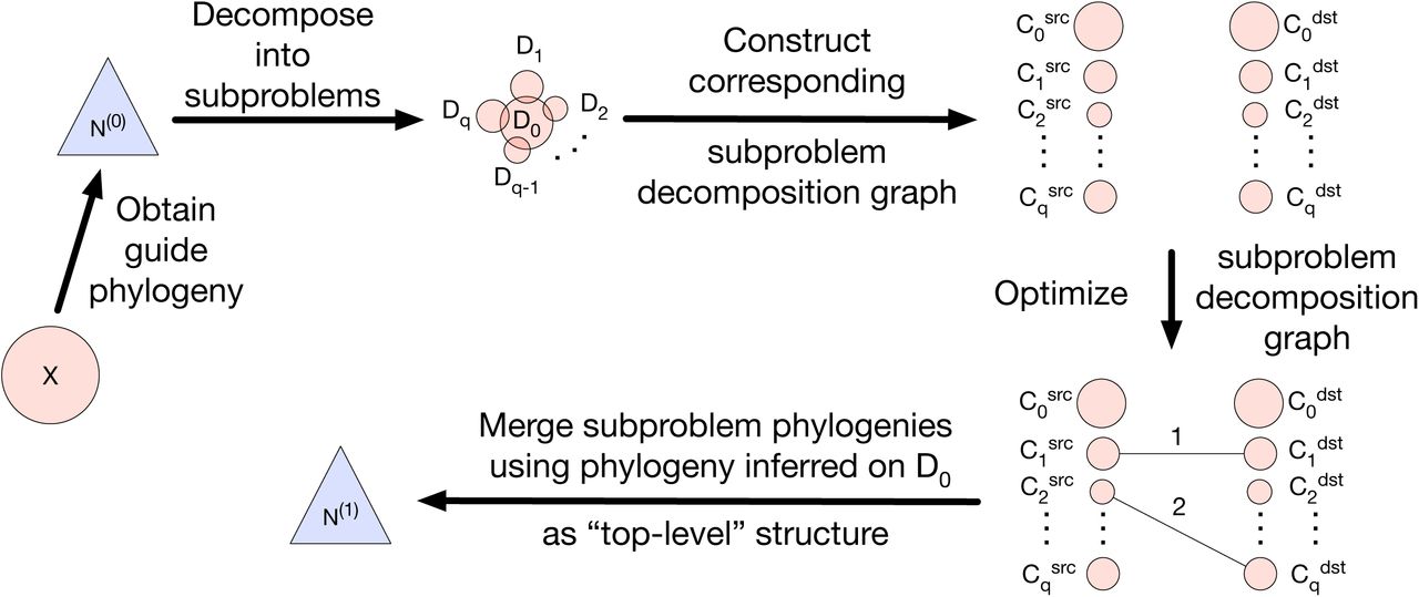
We now describe our new divide-and-conquer algorithm, which we refer to as FastNet. A flowchart of the algorithm is shown in Figure 1.

[scale=0.25]figures/high-level-illustration-of-basic-algorithm.pdf
First, a guide phylogeny N(0) is inferred on the full set of taxa X. Next, the guide phylogeny N(0) is used to decompose X into subproblems {D0, D1, D2, …, Dq–i, Dq} = D. Then, the subproblem decomposition D is used to construct a bipartite graph GD = (VD, ED), which is referred to as the subproblem decomposition graph. The set of vertices VD consist of two partitions: source vertices  where each subproblem Di has a corresponding source vertex
  , and destination vertices
  similarly. The subproblem decomposition graph GD is optimized to infer subproblem phylogenies and reticulations, where the latter are inferred based on the placement of weighted edges e ∈ ED. Finally, the subproblem phylogenies are merged using the phylogeny inferred on D0 as the “top-level” structure.
Step zero: obtaining local gene trees
FastNet is a summary-based method for inferring phylogenetic networks. Each subsequent step of the FastNet algorithm therefore utilizes a set of gene trees G as input, where a gene tree gi ∈ G represents the evolutionary history of each data partition ai. The experiments in our study utilized either true or inferred gene trees as input to summary-based inference methods, including FastNet (see below for details). We used FastTree [28] to perform maximum likelihood estimation of local gene trees. Our study made use of an outgroup, and the unrooted gene trees inferred by FastTree were rooted on the leaf edge corresponding to the outgroup.
Step one: obtaining a guide phylogeny
The subsequent subproblem decomposition step requires a rooted guide phylogeny N(0) The phylogenetic relationships need not be completely accurate. Rather, the guide tree needs to be sufficiently accurate to inform subsequent divide-and-conquer steps. Another essential requirement is that the method used for inferring the guide phylogeny must have reasonable computational requirements.
Based on these criteria, we utilized two different methods to obtain guide phylogenies. We used the parsimony-based algorithm proposed by Yu et al. [21] to infer a rooted species network. The algorithm is implemented in the PhyloNet software package [29]. We refer to this method as MP. In a previous simulation study [15], we found that MP offers a significant runtime advantage relative to other state-of-the-art species network inference methods, but had relatively lower topological accuracy. We also used ASTRAL [30, 31], a state-of-the-art phylogenomic inference method that infers species trees, to infer a guide phylogeny that was a tree rather than a network. A primary reason for the use of species tree inference methods is their computational efficiency relative to state-of-the-art phylogenetic network inference methods. While ASTRAL accurately infers species trees for evolutionary scenarios lacking gene flow, the assumption of tree-like evolution is generally invalid for the computational problem that we consider. As we show in our performance study, our divide-and-conquer approach can still be applied despite this limitation, suggesting that FastNet is robust to guide phylogeny error. Another consideration is that ASTRAL effectively infers an unrooted and undirected species tree. We rooted the species tree using out group rooting.
Step two: subproblem decomposition
The rooted and directed species network N(0) is then used to produce a subproblem decomposition D. The decomposition D consists of a “bottom-level” component and a “top-level” component, which refers to the sub-problem decomposition technique. The bottom-level component is comprised of disjoint subsets Di for 1 ≤ i ≤ q which partition the set of taxa X such that  . We refer to each subset Di as a bottom-level subproblem. The top-level component consists of a top-level subproblem D0 which overlaps each bottom-level subproblem Di where 1 ≤ i ≤ q.
The bottom-level component of the subproblem decomposition is obtained using the following steps. First, for each reticulation node in the network N(0), we delete the incoming edge with lower admixture frequency. Since the resulting phylogeny T(0) contains no reticulation edges and is therefore a tree, removal of any single edge will disconnect the phylogeny into two subtrees; the leaves of the two subtrees will form two subproblems. We extend this observation to obtain decompositions with two or more subproblems. Let S be an open set of nodes in the guide phylogeny T(0) Each node s ∈ S induces a corresponding subproblem Di for 1 ≤ i ≤ q which consists of the taxa corresponding to the leaves that are reachable from s in T(0) Of course, not all decompositions are created equal. In this study, we explore the use of two criteria to evaluate decompositions: the maximum subproblem size cm and a lower bound on the number of subproblems. We addressed the resulting optimization problem using a greedy algorithm. The algorithm is similar to the Center-Tree-i decomposition used by Liu et al. [24] in the context of species tree inference. The main difference is that we parameterize our divide-and-conquer based upon a different set of optimization criteria. The input to our decomposition algorithm is the rooted directed tree T(0) and the parameter cm, which specifies the maximum subproblem size. Our decomposition procedure also stipulates a minimum number of subproblems of 2. Initially the open set S consists of the root node r(T(0)) The open set S is iteratively updated as follows: each iteration greedily selects a node s ∈ S with maximal corresponding subproblem size, the node s is removed from the set S and replaced by its children. Iteration terminates when both decomposition criteria (the maximum subproblem size criterion and the minimum number of subproblems) are satisfied. If no decomposition satisfies the criteria, then the search is restarted using a maximum subproblem size of cm – 1.
In practice, the parameter cm is set to an empirically determined value which is based upon the largest datasets that state-of-the-art methods can analyze accurately within a reasonable timeframe [15]. The output of the search algorithm is effectively a search tree  with a root corresponding to r(T(0)), leaves corresponding to s ∈ S, and the subset of edges in T(0) which connect the root r(T(0)) to the nodes s ∈ S in T(0) The decomposition is obtained by deleting the search tree’s corresponding edge structure in T(0) resulting in q sub-trees which induce bottom-level sub-problems as before.
The top-level component augments the subproblem decomposition with a single top-level subproblem D0 which overlaps each bottom-level subproblem. Phylo-genetic structure inferred on D0 represents ancestral evolutionary relationships among bottom-level sub-problems. Furthermore, overlap between the top-level subproblem D0 and bottom-level subproblems is necessary for the subsequent merge procedure (see “Step four” below). The top-level subproblem D0 contains representative taxa taken from each bottom-level sub-problem Di for 1 ≤ i ≤ q for each bottom-level sub-problem Di, we choose the leaf in T(0) that is closest to the corresponding open set node s ∈ S to represent Di, and the corresponding taxon is included in the top-level subproblem D0.
Step three: subproblem decomposition graph optimization
Tree-based divide-and-conquer approaches reduce evolutionary divergence within sub-problems by effectively partitioning the inference problem based on phylogenetic relationships. Within each part of the true phylogeny corresponding to a subproblem, the space of possible unrooted sub-tree topologies contributes a smaller set of distinct bipartitions (each corresponding to a possible tree edge) that need to be evaluated during search as compared to the full inference problem. The same insight can be applied to reticulation edges as well, except that a given reticulation is not necessarily restricted to a single subproblem.
We address the issue of “inter-subproblem” reticulations through the use of an abstraction which we refer to as a subproblem decomposition graph. A sub-problem decomposition graph GD = (VD, ED) is a bipartite graph where the vertices VD can be partitioned into two sets: a set of source vertices  and a set of destination vertices
  . There is a source vertex
  for each distinct subproblem Di ∈ D where 0 ≤ i ≤ q, and similarly for destination vertices
  . An undirected edge eij ∈ ED connects a source vertex
  to a destination vertex
  where i ≤ j and has a weight
  . If an edge eii connects nodes
  that correspond to the same subproblem Di ∈ D, then the edge weight w(eii) > 0 specifies the number of reticulations in the phylogenetic network to be inferred on subproblem Di; otherwise, a phylogenetic tree is to be inferred on sub-problem Di. If an edge eij connects nodes
  where i < j, then the edge weight w(eij) > 0 specifies the number of “inter-subproblem” reticulations between the subproblems Di and Dj (where an inter-subproblem reticulation is a reticulation with one incoming edge which is incident from the phylogeny to be inferred on subproblem Di and the other incoming edge which is incident from the phylogeny to be inferred on Dj); otherwise, no reticulations are to be inferred between the two subproblems. A subproblem decomposition graph is constrained to have a total number of reticulations such that
  .
.
Given a subproblem decomposition D, FastNet’s search routines make use of the correspondence between a subproblem decomposition graph GD and a multiset with cardinality Cr that is chosen from  elements. Enumeration over corresponding multisets is feasible when the number of subproblems and Cr are sufficiently small (Algorithm 1); otherwise, perturbations of a corresponding multiset can be used as part of a local search heuristic.
1: static variable Cr ⊳Number of reticulations
2: procedure INITIALIZESUBPROBLEMDECOMPOSITIONGRAPH(D)
3: Construct subproblem decomposition graph GD such that ED = {e00} and w(e00) = Cr
4: return (GD)
5: procedure NEXTSUBPROBLEMDECOMPOSITIONGRAPH(GD)
6: Based on edge weights in GD, construct corresponding multiset s of size Cr from  elements
7: if s is last multiset in enumeration over
elements
7: if s is last multiset in enumeration over  possible multisets then
8: return false
9: else
10: Enumerate next multiset s’
11: Update edge weights in GD based on multiset s’
12: return true
possible multisets then
8: return false
9: else
10: Enumerate next multiset s’
11: Update edge weights in GD based on multiset s’
12: return true
A subproblem decomposition graph GD facilitates phylogenetic inference given a subproblem decomposition D. The resulting inference is evaluated with respect to a pseudo-likelihood-based criterion. Pseudocode for the pseudo-likelihood calculation is shown in Algorithm 2.
1: static variable Cr ⊳Number of reticulations
2: static variable G ⊳Set of gene trees
3: procedure COMPUTEOPTIMIZATIONSCOREANDINFERSUBPROBLEMSOLUTIONS(GD, ∆, δ, Ψ, ψ)
4: for i = 0 to q do
5: InferSubnetwork(GD, i, ∆, δ) ⊳Caches inferred network in ∆
⊳Caches inferred network likelihood in δ
6: for i = 0 to q do
7: for j = i + 1 to q do
8: InferSubnetwork(GD, i, j, ∆, δ, Ψ, ψ) ⊳Caches inferred network in Ψ
⊳Caches inferred network likelihood in ψ
9:  ⊳Pseudolikelihood score
⊳ Note that w(GD,i, j) = (eij ∈ E(GD)) ? weight of edge eij: 0
10: return (score)
11:procedure INFERSUBNETWORK(GD, i, ∆, δ)
12: k = (eii ∈ E(GD)) ? w(eii): 0 ⊳eii ∈ E(GD)
13: if defined(∆[i, k]) then
14: return
15: (Ni, score) = F(G|Di, k) ⊳“Boosted” method F(·,·)
⊳G|Di is restriction of G to subproblem taxa Di
16: ∆[i, k] = Ni ⊳Return value by reference to mutable cache ∆
17: δ[i, k] = score ⊳Return value by reference to mutable cache δ
18: procedure INFERSUBNETWORK(GD, i, j, ∆, δ, Ψ, ψ)
19: k = (eij ∈ E(GD)) ? w(eij): 0
20: l = (eii ∈ E(GD)) ? w(eii): 0
21: m = (ejj ∈ E(GD)) ? w(ejj): 0
22: if defined(Ψ [i, j, k, l, m]) then
23: return
24: if not defined(∆[i, l]) then
25: InferSubnetwork(GD, i, ∆, δ)
26: if not defined(∆[j, m]) then
27: InferSubnetwork(GD, j, ∆, δ)
28: Ncherry = ConstructCherry(∆[i, l], ∆[j,m]) ⊳Returns (∆[i, l]:bi, ∆[j,m]:bj);
⊳where bi and bj are inferred using “boosted method” F(·,·)
29: (Nij, score) = AddReticulations(Ncherry, k) ⊳Using “boosted method” F(·,·) to perform constrained search
30: Ψ[i,j, k, l, m] = Nij ⊳Return value by reference to mutable cache Ψ
31: ψ[i, j, k, l, m] = score ⊳Return value by reference to mutable cache ψ
⊳Pseudolikelihood score
⊳ Note that w(GD,i, j) = (eij ∈ E(GD)) ? weight of edge eij: 0
10: return (score)
11:procedure INFERSUBNETWORK(GD, i, ∆, δ)
12: k = (eii ∈ E(GD)) ? w(eii): 0 ⊳eii ∈ E(GD)
13: if defined(∆[i, k]) then
14: return
15: (Ni, score) = F(G|Di, k) ⊳“Boosted” method F(·,·)
⊳G|Di is restriction of G to subproblem taxa Di
16: ∆[i, k] = Ni ⊳Return value by reference to mutable cache ∆
17: δ[i, k] = score ⊳Return value by reference to mutable cache δ
18: procedure INFERSUBNETWORK(GD, i, j, ∆, δ, Ψ, ψ)
19: k = (eij ∈ E(GD)) ? w(eij): 0
20: l = (eii ∈ E(GD)) ? w(eii): 0
21: m = (ejj ∈ E(GD)) ? w(ejj): 0
22: if defined(Ψ [i, j, k, l, m]) then
23: return
24: if not defined(∆[i, l]) then
25: InferSubnetwork(GD, i, ∆, δ)
26: if not defined(∆[j, m]) then
27: InferSubnetwork(GD, j, ∆, δ)
28: Ncherry = ConstructCherry(∆[i, l], ∆[j,m]) ⊳Returns (∆[i, l]:bi, ∆[j,m]:bj);
⊳where bi and bj are inferred using “boosted method” F(·,·)
29: (Nij, score) = AddReticulations(Ncherry, k) ⊳Using “boosted method” F(·,·) to perform constrained search
30: Ψ[i,j, k, l, m] = Nij ⊳Return value by reference to mutable cache Ψ
31: ψ[i, j, k, l, m] = score ⊳Return value by reference to mutable cache ψ
The first step is to analyze each individual subprob-lem Di ∈ D where 0 ≤ i ≤ q. If an edge eii exists, then a phylogenetic network with w(eii) reticulations is inferred on the corresponding subproblem Di; otherwise, a phylogenetic tree is inferred. We utilized MLE, a summary-based MLE method, to perform phylogenetic inference on subproblems, which we refer to as a base method. We note that alternative optimization-based approaches (e.g., other likelihood-based approaches such as MLE-length or pseudo-likelihood-based approaches such as MPL) can be substituted in a straightforward manner.
Next, reticulations are inferred “between” pairs of subproblems as follows. Let Ni and Nj where i ≠ j be the networks inferred on subproblems Di and Dj, respectively, using the above procedure. Construct the cherry (Ni: bi, Nj: bj) ANC; which consists of a new root node ANC with children r(Ni) and r(Nj), where Ni and Nj are respectively retained as sub-phylogenies. Then, infer branch lengths bi and bj and add w(eij) reticulations under the maximum likelihood criterion used by the base method. For pairs of sub-problems not involving the top-level subproblem D0, we used the base method to perform constrained optimization. For pairs of subproblems involving the top-level subproblem D0, we used a greedy heuristic: initial placements were chosen arbitrarily for each reticulation, the source node for each reticulation edge was exhaustively optimized, and then the destination node for each reticulation edge was exhaustively optimized.
Inferred phylogenies and likelihoods were cached to ensure consistency among individual and pairwise sub-problem analyses, which is necessary for the subse-quent merge procedure. Caching also aids computa-tional efficiency.
Finally, the subproblem decomposition graph and as-sociated phylogenetic inferences are evaluated using a pseudolikelihood criterion:
 where w(GD, i, j) is the weight of edge eij if it exists in E(GD) or 0 otherwise, δ[i, w(GD, i, i)] is the cached likelihood for an individual subproblem Di, and ψ[i, j, w(GD, i, j), w(GD, i, i), w(GD, j, j)] is the cached likelihood for a pair of subproblems Di and Dj where i < j. The pseudo-likelihood calculation effectively assumes that subproblems are independent, although they are correlated through connecting edges in the model phylogeny. The choice of optimization criterion in this context represents a tradeoff between efficiency and accuracy, and several other state-of-the-art phylogenetic inference methods also use pseudo-likelihoods to analyze subsets of taxa (e.g., MPL and SNaQ). Other choices are possible. For example, an alternative would be to merge subproblem inferences into a single network hypothesis and calculate its likelihood under the MSNC model.
We optimize subproblem decomposition graphs under the pseudo-likelihood criterion. Exhaustive enumeration of subproblem decomposition graphs is possible for the datasets in our study. Pseudocode to obtain a global optimum is shown in Algorithm 3. For larger datasets with more reticulations, heuristic search techniques can be used to obtain local optima as a more efficient alternative.
1: static variable Cr ⊳Number of reticulations
2: static variable G ⊳Set of gene trees
3: procedure EXHAUSTIVESEARCHFOROPTIMALSUBPROBLEMDECOMPOSITIONGRAPH(D)
4: q = GetNumberOfSubproblems(D)
5: (∆, δ, Ψ, ψ) = InitializeCaches(q, Cr) ⊳Mutable caches persist during subproblem decomposition graph search
6: GD = InitializeSubproblemDecompositionGraph(D)
7:  8: scorebest = ComputeOptimizationScoreAndInferSubproblemSolutions(GD, ∆, δ, Ψ, ψ)
9: while NextSubproblemDecompositionGraph(GD) do
10: score = ComputeOptimizationScoreAndInferSubproblemSolutions(GD, ∆, δ, Ψ, ψ)
11: if score > scorebest then
12:
8: scorebest = ComputeOptimizationScoreAndInferSubproblemSolutions(GD, ∆, δ, Ψ, ψ)
9: while NextSubproblemDecompositionGraph(GD) do
10: score = ComputeOptimizationScoreAndInferSubproblemSolutions(GD, ∆, δ, Ψ, ψ)
11: if score > scorebest then
12:  ⊳Update
13: scorebest = score
14: return(
⊳Update
13: scorebest = score
14: return( , scorebest, ∆, δ, Ψ, ψ)
Step four: merge subproblem phylogenies into a phylogeny on the full set of taxa
Given an optimal subproblem decomposition graph G’D returned by the previous step, the final step of the FastNet algorithm merges the “top-level” phylogenetic structure inferred on D0 and “bottom-level” subproblem phy-logenies Di for 1 ≤ i ≤ q (Algorithm 4). First, the phylogeny inferred on the top-level subproblem D0 serves as the top-level of the output phylogeny N’. Next, the ith taxon in N’ is replaced with the phylogeny inferred on bottom-level subproblem Di, which was cached during the evaluation of G’D. Finally, each “inter-subproblem” reticulation that was inferred for a pair of subproblems Di and Dj where i < j is added to the output phylogeny N’, which is compatible by construction of the decomposition D and the optimal subproblem decomposition graph G’D. The result of the merge procedure is an output phylogeny N’ on the full set of taxa X.
1: static variable Cr ⊳Number of reticulations 2: procedure MERGE(GD, ∆, Ψ) 3: q= GetNumberOfSubproblems(GD) 4: w00 = (e00 ∈ E(GD))? w(e00): 0 5: N = ∆[0, w00] ⊳“Top-level” subproblem phylogeny ⊳ Note that w(e) = (e ∈ E(GD)) ? weight of edge e: 0 6: for i = 1 to q do 7: k = (eii ∈ E(GD)) ? w(eii): 0 8: ReplaceLeafWithSubnetwork(N, GD, i, ∆[i, k]) ⊳Replace ith taxon in “top-level” subproblem D0 9: for i = 1 to q do 10: for j = i + 1 to q do 11: k = (eij ∈ E(GD)) ? w(eij): 0 12: l = (eii ∈ E(GD)) ? w(eii): 0 13: m = (ejj ∈ E(GD)) ? w(ejj): 0 14: if k > 0 then 15: AddCompatibleReticulations(N, GD, i, j, Ψ[i, j, k, l, m]) 16: return(N)
Simulation study
We conducted a simulation study to evaluate the performance of FastNet and existing state-of-the-art methods for phylogenetic network inference. The performance study utilized the following procedures. Detailed commands and software options are given in the Supplementary Material (see Additional File 1).
Simulation of model networks
For each model condition, random model networks were generated using the following procedure. First, r8s version 1.7 [32] was used to simulate random birth-death trees with n taxa where n ∈ {15,20,25,30}, which served as in-group taxa during subsequent analysis. The height of each tree was scaled to 5.0 coalescent units. Next, a time-consistent level-r rooted phylogenetic network [33] was obtained by adding r reticulations to each tree, where r ∈ [1,4]. The procedure for adding a reticulation consists of the following steps: based on a con-sistent timing of events in the tree, (1) choose a time tM uniformly at random between 0 and the tree height, (2) randomly select two tree edges for which corresponding ancestral populations existed during time in-terval [tA, tB] such that tM ∈ [tA, tB], and (3) add a reticulation to connect the pair of tree edges. Finally an outgroup was added to the resulting network at time 15.0.
Reticulations in our study have the same interpretation as in the study of Leaché et al. [34]. Gene flow is modeled using an isolation-with-migration model, where each reticulation is modeled as a unidirectional migration event with rate 5.0 during the time inter-val [tA, tB]. We focus on paraphyletic gene flow as described by Leaché et al.; their study also investigated two other classes of gene flow - isolation-with-migration and ancestral gene flow - both of which involve gene flow between two sister species after divergence. Our simulation study omits these two classes since several existing methods (i.e., MLE and MPL) have issues with identifiability in this context. We note that FastNet makes no assumptions about the type of gene flow to be inferred, and identifiability depends on the model used for inference by FastNet’s base method.
As in the study of Leaché et al., we further classify simulation conditions based on whether gene flow is “non-deep” or “deep” based on topological constraints. Non-deep reticulations involve leaf edges only, and all other reticulations are considered to be deep. Similarly, model conditions with non-deep gene flow have model networks with non-deep reticulations only; all other model conditions include deep reticulations and are referred to as deep.
Simulation of local genealogies and DNA sequences
We used ms [35] to simulate local gene trees for independent and identically distributed (i.i.d.) loci under an extended multi-species coalescent model, where reticulations correspond to migration events as described above. Each coalescent simulation sampled one allele per taxon. The primary experiments in our study simulated 1000 gene trees for each random model network. Our study also investigated data requirements of different methods by including additional datasets where either 200 or 100 gene trees were simulated for each random model network.
Sequence evolution was simulated using seq-gen [36], which takes the local genealogies generated by ms as input and simulates sequence evolution along each genealogy under a finite-sites substitution model. Our simulations utilized the Jukes-Cantor substitution model [37]. We simulated 1000 bp per locus, and the resulting multi-locus sequence alignment had a total length of 1000 kb.
Replicate datasets
A model condition in our study consisted of fixed values for each of the above model parameters. For each model condition, the simulation procedure was repeated twenty times to generate twenty replicate datasets.
Species network inference methods
Our simulation study compared the performance of FastNet against existing methods which were among the fastest and most accurate in our previous performance study of state-of-the-art species network inference methods [15]. Like FastNet, these methods perform summary-based inference - i.e., the input consists of gene trees inferred from sequence alignments for multiple loci, rather than the sequence alignments themselves. The methods are broadly characterized by their statistical optimization criteria: either maximum likelihood or maximum pseudo-likelihood under the multi-species network coalescent (MSNC) model [16]. The maximum likelihood estimation methods consisted of two methods proposed by Yu et al. [14] which are implemented in PhyloNet [29]. One method utilizes gene trees with branch lengths as input observations, whereas the other method considers gene tree topologies only; we refer to the methods as MLE-length and MLE, respectively. Our study also included the pseudo-likelihood-based method of [21], which we refer to as MPL. For each analysis in our study, all species network inference methods - MLE, MLE-length, MPL, and FastNet - were provided with identical inputs.
Our study included two categories of experiments. The “boosting” experiments in our simulation study compared the performance of FastNet against its base method; we refer to all other experiments in our study as “non-boosting”. To make boosting comparisons explicit, each boosting experiment will refer to “Fast-Net(BaseMethod)” which is FastNet run with a specific base method “BaseMethod” - either MLE-length, MLE, or MPL. The input for each boosting experiment consisted of either true or inferred gene trees for all loci. The inferred gene trees were obtained using Fast-Tree [28] with default settings to perform maximum likelihood estimation under the Jukes-Cantor substitution model [37]. The inferred gene trees were rooted using the outgroup. The non-boosting experiments focused on the performance of FastNet using MLE as a base method and inferred gene trees as input, where gene trees were inferred using the same procedure as in the boosting experiments.
Performance measures
The species network inference methods in our study were evaluated using two different criteria. The first criterion was topolog-ical accuracy. For each method, we compared the inferred species phylogeny to the model phylogeny using the tripartition distance [38], which counts the proportion of tripartitions that are not shared between the inferred and model network. The second criterion was computational runtime. All computational analyses were run on computing facilities in Michigan State University’s High Performance Computing Center. We used compute nodes in the intel16 cluster, each of which had a 2.5 GHz Intel Xeon E5-2670v2 processor with 64 GiB of main memory. All replicates completed with memory usage less than 16 GiB.
Empirical datasets
Yeast dataset. We re-analyzed the 23 yeast genomes from the phylogenomic study conducted by Salichos and Rokas [39]. We briefly summarize the procedures that Salichos and Rokas followed to process genomic sequence data. First, orthologs were identified using the Yeast Gene Order Browser (YGOB) [40] and Candida Gene Order Browser (CGOB) [41, 42] synteny databases. Nucleotide sequences were translated into amino acid sequences. The unaligned amino acid sequences were aligned using MAFFT with default settings [43]. Loci were filtered based on alignment length and quality, where the minimum alignment length was 150 bases and at least half of an alignment’s sites consisted of bases only (i.e., had zero indels). The resulting dataset consisted of 1,070 loci.
Unrooted gene trees were inferred using the same procedures as in the study of Salichos and Rokas. For each locus, RAxML [44] was used to perform maximum likelihood estimation of a gene tree under a model of amino acid substitution. The substitution model was selected using ProtTest [45]. Following the procedures of Yu and Nakhleh [13], unrooted gene trees were rooted under the MDC criterion [21] using the species tree reported in [39].
FastNet(MPL) was used to estimate a species network topology using the rooted gene trees as input. We performed fixed-topology optimization of continuous model parameters associated with the species network (i.e. branch length parameters and admixture frequency parameters) using MPL to perform maximum pseudo-likelihood estimation. The corresponding pseudo-likelihoods were compared as part of a slope analysis. As in the study of Yu and Nakhleh, the inferred species networks contained 0, 1, or 2 reticulations.
Mosquito dataset
Our empirical study included a re-analysis of a phylogenomic dataset from the study of Neafsey et al. [46]. We obtained the original version of the dataset from the study authors (D. Neafsey, personal comm.). (An updated version of the dataset can be downloaded from the OrthoDBmoz2 database [46, 47] (http://cegg.unige.ch/orthodbmoz2)). The dataset consists of genomic sequence data for single copy orthologs that are present in 18 anopheline species. A total of 5,099 loci are included. The dataset was known as the “SC Universal” dataset in the study of Neafsey et al. For each locus, RAxML was used to infer an unrooted gene tree under the General Time Reversible (GTR) [48] model of nucleotide substitution with a GAMMA+I model of rate heterogeneity across sites [49]. Unrooted gene trees were rooted using the same procedure as in the yeast dataset re-analysis. Phylogenetic support was evaluated using RAxML to conduct a standard bootstrap analysis with 100 replicates. Gene tree edges with bootstrap support below a threshold of 90% were contracted. Summary-based inference of species networks followed the procedure used in the yeast dataset re-analysis. The inferred species networks contained between 0 and 2 reticulations.
Results
Simulation study
FastNet’s use of phylogenetic divide-and-conquer is compatible with a range of different methods for inferring rooted species networks on subproblems, which we refer to as “base” methods. From a computational perspective, FastNet can be seen as a general-purpose framework for boosting the performance of base methods. We began by assessing the relative performance boost provided by FastNet when used with two different state-of-the-art network inference methods. We evaluated two different aspects of performance: topo-logical error as measured by the tripartition distance [38] between an inferred species network and the model network, and computational runtime. The initial set of boosting experiments focused on species network inference in isolation of upstream inference accuracy by providing true gene trees as input to all of the summary-based inference methods.
In the performance study of Hejase and Liu [15], the probabilistic network inference methods were found to be the most accurate among state-of-the-art methods, and MPL was among the fastest methods in this class. MPL utilized a pseudo-likelihood-based approximation for increased computational efficiency compared with full likelihood methods [13]. However, the tradeoff netted efficiency that was well short of current phylogenomic dataset sizes [15].
Table 1 shows the performance of FastNet(MPL) relative to MPL on model conditions with increasing numbers of taxa and non-deep reticulations. On model conditions with dataset sizes ranging from 15 to 30 taxa and from 1 to 4 reticulations, FastNet(MPL) s improvement in topological error relative to its base method was statistically significant (one-sided pairwise t-test with Benjamini-Hochberg correction for multi-ple tests [50]; α = 0.05 and n = 20) and substantial in magnitude - an absolute improvement that amounted to as much as 41%. Furthermore, the improvement in topological error grew as datasets became larger and involved more reticulations: the largest improvements were seen on the 30-taxon 4-reticulation model condition. Runtime improvements were also statistically significant and represented speedups which amounted as much as a day and a half of runtime.
The relative performance of FastNet(MPL) and MPL is compared on model conditions with 15-30 taxa and 1-4 non-deep reticulations. The performance measures consisted of topological error as measured by the tripartition distance between an inferred species network and the model network and computational runtime in hours. Average (“Avg”) and standard error (“SE”) of FastNet(MPL)’s performance improvement over MPL is reported (n = 20). All methods were provided with true gene trees as input. The statistical significance of FastNet(MPL)’s performance improvement over MPL was assessed using a one-sided t-test. Corrected q-values are reported where multiple test correction was performed using the Benjamini-Hochberg method [50].
Next, we evaluated FastNet’s performance when boosting MLE-length, the most accurate state-of-the-art method from the performance study of He-jase and Liu [15]. On model conditions with non-deep reticulations, FastNet(MLE-length) had a sim-ilar boosting effect as compared to FastNet(MPL) (Table 2). On the 15-taxon single-reticulation model condition, FastNet’s average improvement in topologi-cal error was greater when MLE-length was used as a base method rather than MPL. An even greater improvement in computational runtime was seen: FastNet(MLE-length)’s runtime improvement over MLE-length was over an order of magnitude greater than FastNet(MPL)’s improvement over MPL. As the number of taxa increased from 15 to 20 (but the num-ber of reticulations was fixed to one), FastNet(MLE-length)’s advantage in topological error and run-time relative to its base method nearly doubled. In all cases, FastNet(MLE-length)’s performance im-provements were statistically significant (Benjamini-Hochberg-corrected one-sided pairwise t-test; α = 0.05 and n = 20). Although FastNet(MLE-length) successfully completed analysis of larger datasets (i.e., model conditions with more than 20 taxa and/or more than one reticulation), we were unable to quantify FastNet(MLE-length)’s performance relative to its base method due to MLE-length’s scalability limitations.
The relative performance of FastNet(MLE-length) and MLE-length is compared on model conditions with 15-20 taxa and 1-2 non-deep reticulations. Note that, for the model condition with 20 taxa and 2 reticulations, MLE-length did not finish analysis of any replicates after a week of runtime. Otherwise, table layout and description are identical to Table 1.
We further evaluated FastNet’s performance in the context of additional experimental and methodological considerations. On model conditions with deep gene flow (Table 3), FastNet returned significant improvements in topological accuracy and runtime relative to its base method - either MPL or MLE-length - with one exception: on the 15-taxon single-reticulation model condition, FastNet(MPL) returned a small and statistically insignificant improvement in topological error over MPL. Otherwise, FastNet’s performance boost was robust to the choice of base method. As dataset sizes increased, the average performance boost increased when MPL was the base method; a similar finding applied to runtime improvements when MLE-length was the base method, whereas topolog-ical error improvements were largely unchanged. We note that FastNet’s performance boost was somewhat smaller on model conditions involving deep gene flow as opposed to non-deep gene flow. When maximum-likelihood-estimated gene trees were used as input to summary-based inference in lieu of true gene trees (Table 4), FastNet boosted the topological accuracy and runtime of its base method in all cases and the improvements were statistically significant. As dataset sizes increased, FastNet’s improvement in topological accuracy and runtime grew when MPL was its base method; runtime improvements grew and topologi-cal error improvements were largely unchanged when MLE-length was the base method. Finally, we conducted an additional experiment to evaluate FastNet’s statistical efficiency when given a finite number of observations in terms of the number of loci (Table 5). As the number of loci ranged from genome-scale (i.e., on the order of 1000 loci) to sizes that were smaller by up to an order of magnitude, FastNet’s average topologi-cal error increased by less than 0.02.
The performance improvement of FastNet over its base method (either MPL or MLE-length) is reported for two different performance measures: topological error as measured by tripartition distance and computational runtime in hours. The simulation conditions involved either 15 or 20 taxa and a single deep reticulation. Otherwise, table layout and description are identical to Table 1.
The performance improvement of FastNet over its base method (either MPL or MLE-length) is reported for two different performance measures: topological error as measured by tripartition distance and computational runtime in hours. For each replicate dataset, all summary-based methods were provided with the same input: a set of rooted gene trees that was inferred using FastTree and outgroup rooting (see Methods section for more details). The simulation conditions involved either 15 or 20 taxa and 1-2 non-deep reticulations. Otherwise, table layout and description are identical to Table 1.
The inputs to FastNet(MLE) consisted of gene trees that were inferred using FastTree and outgroup rooting (see Methods section for more details). The simulations sampled between 100 and 1000 loci for a single 20-taxon 1-reticulation model condition involving non-deep gene flow. Topological error was evaluated based upon the tripartition distance between the model phylogeny and the species phylogeny inferred by FastNet(MLE); average (“Avg”) and standard error (“SE”) are shown (n = 20).
Empirical study
Yeast dataset
The yeast dataset in our empirical study was originally published by Salichos and Rokas [39] and re-analyzed by Yu and Nakhleh [13]. Comparing and contrasting the three studies reveals several important areas of strict and majority consensus.
As shown in Supplementary Figure S1, a slope analysis based on pseudo-likelihoods clearly preferred species networks with either one or two reticulations over a species tree hypothesis. Pseudo-likelihoods were calculated using either FastNet’s approach (expression 1) or MPL’s approach. Furthermore, a species network with two reticulations was preferred over a species network with one reticulation. The two-reticulation phy-logeny inferred by FastNet(MPL) is shown in Figure 2. (The one-reticulation phylogeny inferred by Fast-Net(MPL) is shown in Supplementary Figure S2).

[scale=0.45]figures/yeast2-crop.pdf
The yeast dataset was originally published by Salichos and Rokas [39], and Yu and Nakhleh [13] re-analyzed the dataset using MPL. The phylogeny is interpreted and visualized in a manner similar to Figure 3 in [13]. Branch lengths (blue text) are given in coalescent units. Reticulation edges (dashed red lines) are annotated with admixture frequencies (red text). The two-reticulation species network was preferred to phylogenetic hypotheses involving fewer reticulations (see Supplementary Figures S1 and S2 concerning the latter). For reference, the putative whole genome duplication event described by Gabaldón et al. (cf. Figure 1 in [60]) would be placed on the branch incident to the MRCA of the sampled Saccharomyces taxa and Candida glabrata (i.e., the branch with length 0.22). The Dendroscope software package [61] was used in the process of producing the illustration.
The species phylogenies inferred by the three studies largely agreed in terms of topology, with two subtle differences. First, FastNet(MPL) inferred tree edges in the Candida clade (i.e., the Candida lineages described in Figure 1 of [39]) that were identical to those inferred by Salichos and Rokas using concatenated analysis; these tree edges were nearly identical to those inferred by Yu and Nakhleh except for the placement of Candida guiliermondii and Debaryomyces hansenii. Tree edges in the other clade (i.e., the Saccharomyces lineages described in Figure 1 of [39]) were identical across all three studies. Second, the species networks inferred in our study and the study of Yu and Nakhleh largely agreed on the placement of reticulations. Both studies placed one reticulation within the Candida clade. As noted by Yu and Nakhleh, the tree edges spanned by the reticulation had low support in the original study of Salichos and Rokas. In our study, the reticulation is consistent with gene flow involving an unsampled and divergent taxon. Both studies placed another reticulation within the other clade of the species phylogeny. The exact placement, orientation, and admixture frequency of reticulations differed somewhat between our study and the study of Yu and Nakhleh. In particular, the reticulations in our study were relatively deeper within the species phylogeny as compared to the study of Yu and Nakhleh. Based on pseudo-likelihoods calculated using MPL’s optimization criterion, FastNet’s two-reticulation species phy-logeny had a larger pseudo-likelihood compared to the MPL-inferred two-reticulation topology reported by Yu and Nakhleh (Supplementary Table S2); a similar outcome was observed when comparing single-reticulation phylogenies. Of course, we note that Fast-Net addresses a different pseudo-likelihood optimization criterion compared to MPL.
Mosquito dataset
We re-analyzed genomic sequence data that was originally published by Neafsey et al. [46], which is a superset of the data studied by Fontaine et al. [51] and Yu and Nakhleh [13]. The Neaf-sey et al. dataset contains 18 in-group taxa in total - 5 of which are represented in the Fontaine et al. dataset, which has 6 in-group taxa in total.
Consistent with the studies of the smaller six-taxon dataset, a slope analysis of pseudo-likelihoods consistently preferred a species network hypothesis to a species tree hypothesis, and a two-reticulation network was preferred to a single-reticulation network (Supplementary Figure S3). Pseudo-likelihoods were calculated under either FastNet’s optimization criterion (expression 1) or MPL’s optimization criterion.
The two-reticulation species phylogeny inferred by FastNet(MPL) is shown in Figure 3, where reticulations are visualized in a manner similar to [13]. (The single-reticulation species phylogeny inferred by Fast-Net(MPL) is shown in Supplementary Figure S4.) Based on this interpretation, the FastNet-inferred species phylogeny is largely consistent with the other studies in terms of topology. Specifically, the FastNet-inferred topology encodes a tree that refines the species tree reported by Neafsey et al., which is fully resolved except for the clade corresponding to the Gambiae complex. Focusing on the 5 taxa within the Gambiae complex, the species phylogeny inferred by FastNet on the Neafsey et al. dataset has tree edges which agree with the species phylogeny reported by Fontaine et al. (shown as Figure 1C in [51]) and the MLE-inferred species phylogeny reported by Wen et al. [52], both of which were inferred using the 6-taxon Fontaine et al. dataset. We note that other interpretations are possible (cf. Figure 7 in [52]). Similar to the studies of Wen et al. and Fontaine et al., FastNet(MPL) infers gene flow within the clade corresponding to the Gam-biae complex. The above interpretation indicates that the FastNet-inferred reticulation involves the A. gam-biae lineage and the MRCA of A. quadriannulatus and A. arabiensis. The FastNet-inferred species phylogeny has an additional reticulation that is ancestral to those reported on the smaller Fontaine et al. dataset. This finding is consistent with the study of Wen et al., which inferred an ancestral reticulation involving an unsam-pled basal taxon based on analysis of the X chromosome (see Figures 4D and 7B in [52]). Due to the larger set of taxa used in our study, FastNet(MPL) inference was able to pinpoint the source endpoints for this reticulation within the expanded Anopheles phylogeny.

[scale=0.45]figures/mosquito2.pdf
The mosquito dataset was originally published by Neasey et al. [46]. The two-reticulation species network was preferred to phylogenetic hypotheses involving fewer reticulations (see Supplementary Figures S3 and S4 concerning the latter). Otherwise, figure layout and description are identical to Figure 2.
Discussion
Simulation study
Relative to the state-of-the-art methods that served as base methods, FastNet consistently returned sizeable and statistically significant improvements in topological error and computational runtime across a range of dataset scales and gene flow scenarios. There was only a single experimental condition where comparable error without statistically significant improvements was seen. This exception occurred when FastNet was used to boost a relatively inaccurate base method (MPL) on the smallest dataset sizes in our study and with deep gene flow; even still, large and statistically significant runtime improvements were seen in this case. In contrast, with a more accurate base method (i.e., MLE-length), large and statistically significant performance improvements were seen throughout our simulation study.
FastNet’s boosting effect on topological error and runtime were robust to several different experimental and design factors. The boosting performance obtained using different base methods - one with lower computational requirements but higher topological error relative to a more computationally intensive alternative - suggests that, while accuracy improvements can be obtained even using less accurate subproblem inference, even greater accuracy improvements can be obtained when reasonably accurate subproblem phylo-genies can be inferred. We note that the base methods were run in default mode. More intensive search settings for each base method’s optimization procedures may allow a tradeoff between topological accuracy and computational runtime. We stress that our goal was not to make specific recommendations about the nuances of running the base methods. Rather, FastNet’s divide-and-conquer framework can be viewed as orthogonal to the specific algorithmic approaches utilized by a base method. In this sense, improvements to the latter accrue to the former in a straightforward and modular manner. Furthermore, FastNet’s performance effect was robust to gene tree error and varying numbers of observed loci.
The biggest performance gains were observed on the largest, most challenging datasets - dataset scales which are becoming increasingly common in systematic studies. The findings in our earlier performance study [15] suggest that, given weeks of computational runtime, even the fastest statistical methods (including MPL) would not complete analysis of datasets with more than 50 taxa or so and several reticulations. In comparison to MPL, FastNet(MPL) was faster by more than an order of magnitude on the largest datasets in our study, and we predict that Fast-Net(MPL) would readily scale to datasets with many dozens of taxa and multiple reticulations.
Yeast dataset re-analysis. FastNet analyses of the genomic sequence dataset from the study of Salichos and Rokas [39] indicated that a yeast phylogeny involving gene flow and incomplete lineage sorting (ILS) is a more plausible hypothesis than one involving ILS alone. Our finding is consistent with the study of Yu and Nakhleh [13], and contrasts with the conclusions of Salichos and Rokas. Specifically, the distribution of observed local genealogies better reflects a multi-species network coalescent model [16] as opposed to a basic multi-species coalescent model. The former model’s local genealogical distribution can be seen as a specific distortion of the latter model’s distribution that is obtained using one or a few reticulations. Furthermore, our study and the study of Yu and Nakhleh found that a species phylogeny with two reticulations is preferred to one with a single reticulation.
The topologies of the species phylogenies in the three studies are largely identical, with two main differences. First, all three studies agree on tree edges, except for the placement of C. guiliermondii and D. hansenii. Our study agrees with the study of Salichos and Rokas regarding the placement of these two taxa, and differs from the study of Yu and Nakhleh. Second, there were some differences between our study and the study of Yu and Nakhleh regarding the placement of reticulations. In both studies, one reticulation involves Candida lineages and the other involves Saccharomyces lineages. The two reticulations were deeper in the species phylogeny as compared to those inferred by Yu and Nakhleh. Our findings are consistent with the deeper hybridization events hypothesized by another recent phylogenomic study [53]. We note that neither our study nor the study of Yu and Nakhleh reconstructed recent hybridizations which have been described in the literature. Some of the putative hybridizations involve species which are not sampled in our dataset (e.g., S. bayanus is thought to be a hybrid of S. cerevisiae and two other taxa that are not sampled in our dataset [54]) and present identifiability issues noted above. It’s also possible that other hybridization and/or intro-gression events occurred during yeast genome evolution, requiring the exploration of more complex phy-logenetic hypotheses (i.e., networks with more reticulations) than those explored in either study. We also note that Salichos and Rokas filtered the loci used in their study to account for hidden paralogy as well as horizontal gene transfer and other types of gene flow (cf. “Data matrix construction” in Methods section of [39]). Salichos and Rokas assert that hybridization and introgression involving the filtered loci would require a specific set of evolutionary outcomes which is thought to be relatively rare. The findings from our study and the study of Yu and Nakhleh show strong support for an alternative hypothesis that runs contrary to this conventional wisdom. As suggested by Wolfe [55], a more nuanced understanding of the interplay between gene flow and other complex evolutionary events such as whole-genome duplication [56-58] awaits further phylogenomic study.
Finally, FastNet-inferred species networks were more optimal than MPL-inferred species networks when compared under MPL’s statistical criterion (with the caveat that FastNet’s subproblem decomposition graph optimization makes use of a different statistical criterion). These findings suggest that phylogenetic divide-and-conquer may prove to be a useful technique for network search under a variety of different optimization criteria.
Mosquito dataset re-analysis
Our re-analysis of the 18-taxon dataset published by Neafsey et al. [46] confirmed the historical introgression in the Anopheles phylogeny that was detected by Fontaine et al. [51] and Wen et al. [52] by analyzing a smaller 6-taxon dataset. The larger dataset was nearly a superset of the smaller dataset - only a single taxon in the Gam-biae complex was present in the latter but not in the former. The FastNet analysis returned a network with tree edges which are compatible with the species tree reported in Neafsey et al.’s study. When restricted to shared taxa within the Gambiae complex, the FastNet phylogeny has an interpretation which agrees with the consensus tree reported by Fontaine et al. and Wen et al.’s findings. The reticulation scenarios inferred by the three studies were generally in agreement. FastNet analysis recovered a reticulation within the Gambiae complex, which agrees with the findings of Fontaine et al. and Wen et al.; the FastNet-inferred species phy-logeny also includes another reticulation ancestral to the Gambiae clade, which is consistent with one of the hypotheses explored in the study of Wen et al. (cf. Figures 4D and 7B in [52]). The expanded superset of in-group taxa used in our study enables us to place all source nodes of the additional reticulation within the expanded Anopheles phylogeny. We note that Fontaine et al.’s geography-based subset analysis suggests both recent and ancient signatures of in-trogression. Furthermore, there is evidence of ancient introgression based on low-read-depth re-sequencing studies of natural populations. We attribute minor variations among inferred reticulations to methodological differences among the three studies. The taxa examined by the three studies are different: our study examines three times the number of taxa than are present in the other studies. Apart from providing a case study for large-scale phylogenetic network estimation, greater taxon sampling in phylogenomic studies potentially provides additional phylogenetic signal relative to small-scale sampling. Other methodological differences include gene tree rooting and the approach used for selection and/or filtering genomic loci.
Conclusion
In this study, we introduced FastNet, a new computational method for inferring phylogenetic networks from large-scale genomic sequence datasets. FastNet utilizes a divide-and-conquer algorithm to constrain two different aspects of scale: the number of taxa and evolutionary divergence. We evaluated the performance of FastNet in comparison to state-of-the-art phyloge-netic network inference methods. We found that Fast-Net improves upon existing methods in terms of computational efficiency and topological accuracy. On the largest datasets explored in our study, the use of the FastNet algorithm as a boosting framework enabled runtime speedups that were over an order of magnitude faster than standalone analysis using a state-of-the-art method. Furthermore, FastNet returned comparable or typically improved topological accuracy compared to the state-of-the-art-methods that were used as its base method.
Future enhancements to FastNet’s algorithmic design are anticipated to yield additional performance improvements. Here we highlight several possibilities. First, recursive application of phylogenetic divide-and-conquer will allow “load balancing” of subproblem size and divergence, enabling further scalability gains. Second, the use of a better guide phylogeny should yield an improved subproblem decomposition and better subproblem decomposition graph optimization. The FastNet-inferred species phylogeny would be a suitable choice in this regard, as demonstrated by the topolog-ical error comparisons in our performance study. This insight naturally suggests an iterative approach: the output phylogeny from one iteration of the FastNet algorithm would be used as the guide phylogeny for a subsequent iteration of the algorithm. Iteration would continue until convergence under a suitable criterion (e.g., FastNet’s pseudo-likelihood criterion). Third, we note that the FastNet algorithm is pleasantly par-allelizable (as are some of the other state-of-the-art methods explored in our study).
We conclude with some parting thoughts about the computational problem of phylogenetic network inference. In today’s post-genomic era, current trends in biomolecular sequence technologies suggest that even the scalability advance set forth in this study will not suffice for near future studies. There is a critical need for new phylogenomic methodologies which can infer species networks involving thousands of taxa or more. Another important issue involves appropriate representations for phylogenies involving both vertical divergence and horizontal gene flow. We would argue that, in explicit phylogenetic network representations, exact placement of the endpoints of reticulation edges may be difficult in some cases, whereas a summary-based localization may be tractable and almost as informative (cf. Figure 3 in [14]). We believe that Fast-Net’s subproblem decomposition graph optimization suggests a way forward via alternative phylogenetic representations that summarize gene flow within “regions” of a phylogeny. One possibility would be to generalize tree-based concordance factors [59] for this purpose.
Availability of data and materials
Software source code and datasets generated and/or analyzed in our study are publicly available under open access licenses. A snapshot of the data and electronic materials is available from figshare under the GNU General Public License version 3 (GPLv3); the associated DOI is 10.6084/m9.figshare.5785479. Updated versions of the FastNet software as well as datasets associated with our study can be found in a GitLab repository that is hosted by Michigan State University. The repository can be accessed at https://gitlab.msu.edu/liulab/FastNet.data.scripts.
Repository files are distributed on an open access basis under the terms of the GNU General Public License version 3 (https://www.gnu.org/licenses/gpl-3.0.txt) and the Creative Commons Attribution-ShareAlike 4.0 International license (https://creativecommons.org/licenses/by-sa/4.0/).
Competing interests
The authors declare that they have no competing interests.
Author’s contributions
Conceived and designed the experiments: HAH KJL. Implemented software tools: HAH. Performed simulation study experiments: HAH. Performed empirical study experiments: HAH NVP. Analyzed the data: GMB HAH KJL NVP. Wrote the paper: GMB HAH KJL NVP. All of the authors have read and approved the final manuscript.
Additional Files
Additional file 1 - Supplementary Material
This file contains supplementary text, supplementary figures, and supplementary tables.
Acknowledgements
We gratefully acknowledge the following support: National Science Foundation (NSF) grants no. CCF-1565719 (to KJL), CCF-1714417 (to KJL), and DEB-1737898 (to GMB and KJL), grants from the BEACON Center for the Study of Evolution in Action (NSF STC Cooperative Agreement DBI-093954) to GMB and KJL, and Michigan State University (MSU) faculty startup funds (to GMB and to KJL). Computational analyses were performed on computing facilities maintained by MSU’s High Performance Computing Center (HPCC). We would also like to acknowledge Daniel Neafsey for kindly sending us a processed version of the genomic sequence dataset from [46].
References


