

Abstract
This research was facilitated by the Social Science Genetic Association Consortium (SSGAC) and by the research group on genetic and social causes of life chances at the Zentrum für interdisplinäre Forschung (ZiF) Bielefeld. Data analyses make use of the UK Biobank resource under application number 11425. We acknowledge data access from the Genetic Investigation of ANthropometric Traits Consortium (GIANT). We used data from the Health and Retirement Study (HRS), which is supported by the National Institute on Aging (NIA U01AG009740, RC2 AG036495, RC4 AG039029). HRS genotype data can be accessed via the database of Genotypes and Phenotypes (dbGaP, accession number phs000428.v1.p1). Researchers who wish to link genetic data with other HRS measures that are not in dbGaP, such as educational attainment, must apply for access from HRS. We are very grateful to Richard Karlsson Linnér for help with the GWAS analyses in the UK Biobank and to Aysu Okbay for providing us with subsets of the GWAS meta-analysis on educational attainment. We thank Patrick Turley, Daniel J. Benjamin, Jonathan Beauchamp, Niels Rietveld, Eric Slob, Hans van Kippersluis, Benjamin Domingue, and Lisbeth Trille Loft for productive discussions and comments on earlier versions of the manuscript. The study was supported by funding from an ERC Consolidator Grant (647648 EdGe, Philipp D. Koellinger).
Abstract We introduce Genetic Instrumental Variables (GIV) regression – a method to estimate causal effects in non-experimental data with many possible applications in the social sciences and epidemiology. In non-experimental data, genetic correlation between the outcome and the exposure of interest is a source of bias. Instrumental variable (IV) regression is a potential solution, but valid instruments are scarce. Existing literature proposes to use genes related to the exposure as instruments (i.e. Mendelian Ran-domization – MR), but this approach is problematic due to possible pleiotropic effects of genes that can violate the assumptions of IV regression. In contrast, GIV regression provides accurate estimates for the causal effect of the exposure and gene-environment interactions involving the exposure under less restrictive assumptions than for MR. As a valuable byproduct, GIV regression also provides accurate estimates of the chip heritability of the outcome variable. GIV regression uses polygenic scores (PGS) for the exposure and the outcome of interest, both of which can be constructed from genome-wide association study (GWAS) results. By splitting the GWAS sample for the outcome into non-overlapping subsamples, we obtain multiple indicators of the outcome PGS that can be used as instruments for each other. In two empirical applications, we demonstrate that our approach produces reasonable estimates of the chip heritability of educational attainment (EA) and, unlike the results using MR, GIV regression estimates find that the positive relationship between body height and EA is primarily due to genetic confounds that have pleiotropic effects on both traits.
Introduction
A major challenge in the social sciences and in epidemiology is the identification of causal effects in non-experimental data. In these disciplines, ethical and legal considerations along with practical constraints often preclude the use of experiments to randomize the assignment of observations between treatment and control groups or to carry out such experiments in samples that represent the relevant population [1]. Instead, many important questions are studied in field data which make it difficult to discern between causal effects and (spurious) correlations that are induced by unobserved factors [2]. Obviously, confusing correlation with causation is not only a conceptual error, it can also lead to ineffective or even harmful recommendations, treatments, and policies, as well as a significant waste of resources (e.g., as in [3]).
One important source of bias in field data is genetic effects: Twin studies [4] as well as methods based on molecular genetic data [5, 6] can be used to estimate the proportion of variance in a trait that is due to the linear genetic effects (so-called narrow-sense heritability). Using these and related methods, an overwhelming body of literature demonstrates that almost all important human traits, behaviors, and health outcomes are influenced both by genetic predisposition as well as environmental factors ([7, 8, 9]). Most of these traits are “genetically complex”, which means that the observed heritability is due to the accumulation of effects from a very large number of genes that each have a small, often statistically insignificant, influence [10]. Furthermore, genes often influence several seemingly unrelated traits (i.e. they have “pleiotropic effects”) [11] and genetic correlations between many traits have been convincingly demonstrated [12], giving rise to unobserved variable bias in field studies that do not control for the genetic predisposition of individuals for the exposure and the outcome of interest.
One popular strategy to isolate causal effects in non-experimental data is to use instrumental variables (IVs) which “purge” the exposure of its correlation with the error term in the regression [13]. IVs need to satisfy two important assumptions. First, they need to be correlated with the exposure of interest conditional on the other control variables in the regression (i.e. IVs need to be “relevant”). Second, they need to be independent of the error term of the regression conditional on the other control variables and produce their correlation with the outcome solely through their effect on the exposure. In practice, finding valid IVs that satisfy both requirements is difficult. In particular, the second requirement (the socalled exclusion restriction) is challenging.
Epidemiologists have proposed to use genetic information to construct IVs and termed this approach Mendelian Randomization (MR) [14, 15, 16, 17]. The idea is in principle appealing because genotypes are randomized in the production of gametes by the process of meiosis. Thus, conditional on the genotype of the parents, the genotype of the offspring are the result of a random draw. So if it would be known which genes affect the exposure, it may be possible to use them as IVs to identify the causal influence of the exposure on some outcome of interest. Yet, there are four challenges to this idea. First, we need to know which genes affect the exposure and isolate true genetic effects from environmental confounds that are correlated with ancestry. Second, if the exposure is a genetically complex trait, any gene by it-self will only capture a very small part of the variance in the trait, which leads to the well-known problem of weak instruments [18, 19]. Third, genotypes are only randomly assigned conditional on the genotype of the parents. Unless it is possible to control for the genotype of the parents, the genotype of the off-spring is not random and correlates with everything that the genotypes of the parents correlate with (e.g. parental environment, personality, and habits) [20]. Fourth, the function of most genes is not completely understood. Therefore, it is difficult to rule out direct pleiotropic effects of genes on the exposure and the outcome, which would violate the exclusion restriction [16].
Recent advances in complex trait genetics make it possible to address the first two challenges of MR. Array-based genotyping technologies have made the collection of genetic data fast and cheap. As a result, very large datasets are now available to study the genetic architecture of many human traits and a plethora of robust, replicable genetic associations has recently been reported in large-scale genome-wide association studies (GWAS) [21]. These results begin to shed a light on the genetic architecture that is driving the heritability of traits such as body height [22], BMI [23], schizophrenia [24], Alzheimer’s disease [25], depression [26], or educational attainment (EA) [27]. High quality GWASs use several strategies to control for genetic structure in the population and indeed, empirical evidence suggests that the vast majority of the reported genetic associations for many traits is not confounded by ancestry [28, 29, 30, 31]. Furthermore, so-called polygenic scores (PGS) have become the favored tool for summarizing the genetic predispositions for genetically complex traits [32, 33, ?, 27]. PGS are linear indices that aggregate the effects of all currently measured genetic variants (typically single nucleotide polymorphisms, a.k.a. SNPs), and recent studies demonstrate the ability of PGS to predict genetically complex outcomes such as height, BMI, schizophrenia, and EA [34, 22, 23, 24, ?]. For example, a polygenic score for EA currently captures 4-6% of the variance in the trait and replicates extremely well across different hold-out samples [27]. Although PGS still capture substantially less of the variation in traits than suggested by their heritability [35] (an issue we return to below), PGS capture a much larger share of the variance of genetically complex traits than individual genetic markers. The third challenge could in principle be addressed if the genotypes of the parents and the offspring are observed (e.g. in a large sample of trios) or by using large samples of dizygotic twins where the genetic differences between siblings are random draws from the parent’s genotypes. However, the fourth challenge (i.e. pleiotropy) remains a serious obstacle despite recent efforts to relax the exogeneity assumptions in MR ([36, 37]).
Here, we present a novel method that we call Genetic Instrumental Variables (GIV) regression that can be implemented using widely available statistical software. In contrast to MR, GIV regression does not require strong assumptions about the causal mechanism of genes because it effectively controls for possible pleiotropic effects of genes. In particular, GIV regression is based on the insight that adding the true PGS for the outcome to a regression model would effectively eliminate bias arising from a genetic correlation between the outcome and an exposure of interest. Furthermore, we argue that the attenuated predictive accuracy of PGS is conceptually similar to the well-known problem of measurement error in regression analysis. Instrumental variable (IV) techniques can correct attenuation bias in regression coefficient estimates that results from measurement error [38]. We argue that it is possible to obtain a valid IV for a PGS by randomly splitting the GWAS sample that was used for its construction. Typically, a GWAS is used to estimate the effects of individual SNPs in a discovery sample. Then, the estimated effects are utilized as weights for the genetic data in an independent prediction sample. By splitting the GWAS sample into independent subsamples, one can obtain several PGS (i.e. multiple indicators) in the prediction sample. Each will have even lower predictive accuracy than the original score due to the smaller GWAS subsamples used in their construction, but these multiple indicators can be used as IVs for each other, and the instruments will satisfy the assumptions of IV regression to the extent that the measurement errors (the difference between the true and calculated PGS) are uncorrelated.
We show that it is possible under plausible assumptions to obtain consistent estimates of the narrow-sense heritability of a trait by using IV regression that utilizes two PGS that were constructed this way. Then we extend the idea to the problem of estimating causal effects in non-experimental data. We argue that using multiple indicators of the PGS of the outcome together with a PGS for the exposure produce IVs that come reasonably close to satisfying the assumptions of IV regression. Finally, we demonstrate how our approach can be straightforwardly extended to obtain causal estimates of gene-environment interactions (GxE) on outcomes.
We begin by laying out the assumptions of our approach and prove that GIV regression yields consistent estimates for the effect of the PGS on the outcome variable, when the other covariates in the model are exogenous and when the true PGS is uncorrelated with the error term net of the included covariates. We then turn to the more complex case of when a regressor of interest (T) is potentially correlated with unobserved variables in the error term because of pleiotropy, and we show that the bias under these assumptions with GIV regression is generally smaller than with OLS, MR, or what we will term an enhanced version of MR (EMR). We then use simulations to test how our approach behaves in finite sample under plausible assumptions about genetic correlations and then show how sensitive our method is to violations of the assumptions in comparison to MR and EMR.
Next, we demonstrate the practical usefulness of our approach in empirical applications using the publicly available Health and Retirement Study [39]. First, we demonstrate that a consistent estimate of the so-called chip heritability [35] of EA can be obtained with our method. Then, we estimate the effects of body height on EA. As a “negative control,” we check whether our method finds a causal effect of EA on body height (it should not). 1
Theory
Assumptions
The methods we describe builds on the standard identifying assumptions of IV regression [13]. In the context of our approach, this implies four specific conditions:
Complete genetic information: The available genetic data include all variants that influence the variable(s) of interest.
Genetic effects are linear: All genetic variants influence the variable(s) of interest via additive linear effects. Thus, there are no genetic interactions (i.e. epistasis) or dominant alleles.
Genome-wide association studies successfully control for population structure: In other words, the available regression coefficients for the genetic variants are not systematically biased by omitted variables that describe the genetic ancestry of the population. Failure to control for population structure can lead to spurious genetic associations [20].
It is possible to divide GWAS samples into non-overlapping sub-samples drawn from the same population as the sample used for analysis.
Estimating narrow-sense SNP heritability from polygenic scores
Under these assumptions, consistent estimates of the chip heritability of a trait2 can be obtained from polygenic scores (for full details, see Supporting Information section 2). If y is the outcome variable, X is a vector of exogenous control variables, and  is a summary measure of genetic tendency for y, then one can write
 where G is an n×m matrix of genetic markers, and ζ is the m×1 vector of SNP effect sizes, where the number of SNPs is typically in the millions. If the true effects of each SNP on the outcome were known, the true genetic tendency
  would be expressed by the PGS for y, and the marginal R2 of
  in equation 1 would be the chip heritability of the trait. In practice, GWAS results are obtained from finite sample sizes that only yield noisy estimates of the true effects of each SNP. Thus, a PGS constructed from GWAS results typically captures far less of the variation in y than suggested by the chip heritability of the trait ([40]; [33]; [35]). This is akin to the well-known attenuation bias resulting from measurement error [41]. We refer to the estimate of the PGS from available GWAS data as Sy, where
 and substitute Sy for
  in equation 1. The variance of a trait that is captured by its available PGS increases with the available GWAS sample size to estimate ζy and converges to the SNP-based narrow-sense heritability of the trait at the limit if all relevant genetic markers were included in the GWAS and if the GWAS sample size were sufficiently large [35].
It has long been understood that multiple indicators can, under certain conditions, provide a strategy to correct regression estimates for attenuation from measurement error ([42]; [43]). IV regression using estimation strategies such as two stage least squares (2SLS) and limited information maximum likelihood (LIML) will provide a consistent estimate for the regression coefficient of a variable that is measured with error if certain assumptions are satisfied ([38]; [44]): (1) The IV is correlated with the problem regressor, and (2) conditional on the variables included in the regression, the IV does not directly cause the outcome variable, and it is not correlated with any of the unobserved variables that cause the outcome variable [38]. In general, these assumptions are difficult to satisfy. In the present case, however, GWAS summary statistics can be used in a way that comes close enough to meeting these conditions to measurably improve results obtainable from standard regression.
The most straightforward solution to the problem of attenuation bias is to obtain multiple indicators of the PGS by splitting the GWAS discovery sample for y into two mutually exclusive subsamples. This produces noisier estimates of  , with lower predictive accuracy, but the multiple indicators can be used as IVs for each other (SI appendix). Standard 2SLS regression using Sy1 as an instrument for Sy2 will then recovered a consistent estimate of γ in equation 1.
Reducing bias arising from genetic correlation between exposure and outcome
The logic from above can be extended to situations where the question of interest is not the chip heritability of y per se, but rather the effect of some non-randomized exposure on y (e.g. a behavioral or environmental variable, or a non-randomized treatment due to policy or medical interventions). We can rewrite equation 1 by adding a treatment variable of interest T, such that
 where, for example, y is EA and T is body height. In each case, it is presumed that the outcome variable is to some extent caused by genetic factors, and the concern is that the genetic propensity for the outcome variable
  is also correlated with the exposure represented by T in equation (3). If
  is not observed and controlled for in equation 3, δ̂ will be a biased estimate of the effect of T on y.3
In standard Mendelian randomization (MR), a measure of genetic tendency (ST) for a behavior of interest (T in equation 3) is used as an IV in an effort to purge δ of bias that arises from correlation between T and unobservable variables in the disturbance term under the argument that the genetic tendency variable, e.g., the measured PGS ST, is exogenous ([46];[44]). One such example would be the use of a PGS for height as an instrument for height in a regression of EA on height. The problem with this approach is that the PGS for height will fail to satisfy the exclusion restriction if (some) of the genes affecting height also have a direct effect on EA (e.g. via healthy cell growth and metabolism) or if they are correlated with unmeasured environmental factors that affect EA.4 Note that this problem arising from pleiotropic effects of genes is not solved even if infinitely large GWAS samples would be available.
The multiple indicator strategy described above provides multiple approaches for addressing the bias in MR. If the genetic propensity for y could be directly controlled in the regression, MR would provide less biased estimates of the effect of T. We refer to the combined use of Sy1 as a control and ST as an IV as “enhanced Mendelian Randomization” (EMR). However, controlling for Sy1 as a proxy for  is not adequate, both because it leaves a component of
  in the error term which causes the exclusion restriction assumption of MR to fail, and because the bias in the estimated coefficient of Sy1 also produces bias in the estimated coefficient of T. The bias arising from the use of a proxy for
  is a form of omitted variable bias (SI appendix).
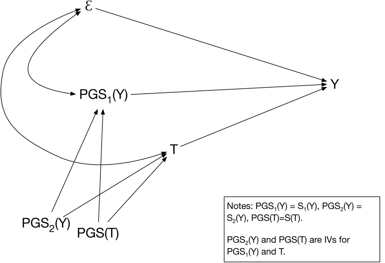
Violation of the exclusion restriction due to genetic correlation is potentially solved (or at least is less severe) when a third indicator of the PGS for y, i.e., Sy3 is used to instrument simultaneously both Sy1 and T in equation 1. However, the practical problem with using two indicators  as the sole instruments is that their mutual correlation will be relatively high (depending on their reliability) and they are weak instruments for T. As a practical strategy, the best solution is arguably to use ST along with Sy2 (or Sy2 and Sy3) as instruments for Sy1 and T. ST will still violate the exclusion restriction to the extent that it is correlated with Guy1. However, the extent of the violation will be reduced by the presence of Sy1 in the regression. Arguably a strategy that both reduces the correlation between ST and E (through the inclusion of Sy1 in the model) and eliminates or greatly reduces omitted variable bias through the inclusion of an instrument for Sy1 in the first stage equation will outperform MR in the estimation of a consistent effect of T that is purged of genetic correlation. Figure 1 illustrates the GIV regression strategy we propose.

Genetic Instrumental Variables (GIV) regression
As noted above, if not all relevant genetic effects are contained in the PGS (e.g. interaction effects, structural variants, or rare alleles may be missing given currently available GWAS data), the PGS instruments above will not perfectly satisfy the exclusion restriction to the extent that  is correlated with the omitted genetic variables. However, the above approach would generally be expected to reduce bias due to genetic correlation, given that a large fraction of heritability can be attributed to linear effects of common SNPs that are well tagged by currently available genotyping arrays [35, 47, 34, 48]). See the SI appendix for details.
Gene-environment interactions
We next generalize equation (3) to the case of gene-environment interactions, where the effect of T varies with the PGS. In principle, these interactions could be extremely complicated and so for practical reasons, swe focus her on obtaining plausible estimates of the linear interaction between  and T. We rewrite equation (3) as
 Now there are three endogenous variables, T, Sy1, and T Sy1. Also the disturbance term has now been elaborated to include a term that is a function of T, and so an additional PGS for y is needed as an additional instrumental variable. This additional PGS for y will allow the use of IV regression to estimate δ2. In the simulations described in section SI 3.3 (see SI Figure 14), GIV regression performs better than OLS, MR, or EMR in estimating the parameters of equation 4. Of course, the term
  may not fully capture all gene-environment interactions involving T or other environmental variables. Correlations between the IVs and variables in the error term of equation 4 will violate the assumptions of IV regression. We address issues of violated assumptions below.

Model with measurement errors and no additional endogeneity and methods 1,2,3,6 (see main text)
Estimated coefficients for model A, using various methods. The mean of the simulations for each method is shown, together with simulated 95% confidence interval is shown. The simulations are based on a sample of 8,600, assuming 300,000 independent SNPs, a heritability of 0.2 and 0.55 for y and T respectively, a genetic correlation of 0.15, a coefficient of 0.15 for effect of T on y and a correlation of 0.4 between the error terms in y and T.

Model with measurement errors and no additional endogeneity and methods 1,2,4,5 (see main text)
Estimated coefficients for model A, using various methods. The mean of the simulations for each method is shown, together with simulated 95% confidence interval is shown. The simulations are based on a sample of 8,600, assuming 300,000 independent SNPs, a heritability of 0.2 and 0.55 for y and T respectively, a genetic correlation of 0.15, a coefficient of 0.15 for effect of T on y and a correlation of 0.4 between the error terms in y and T. Note that for method 5 the confidence bounds are outside of the figure.

Model with measurement errors and no additional endogeneity and methods 1,5,6,7 (see main text)
Estimated coefficients for model A, using various methods. The mean of the simulations for each method is shown, together with simulated 95% confidence interval is shown. The simulations are based on a sample of 8,600, assuming 300,000 independent SNPs, a heritability of 0.2 and 0.55 for y and T respectively, a genetic correlation of 0.15, a coefficient of 0.15 for effect of T on y and a correlation of 0.4 between the error terms in y and T. Note that for method 5 the confidence bounds are outside of the figure.

Model with measurement errors, additional endogeneity, and methods 1,2,4,7 (see main text)
Estimated coefficients for model A, using various methods. The mean of the simulations for each method is shown, together with simulated 95% confidence interval is shown. The simulations are based on a sample of 8,600, assuming 300,000 independent SNPs, a heritability of 0.2 and 0.55 for y and T respectively, a genetic correlation of 0.15, a coefficient of 0.15 for effect of T on y and a correlation of 0.4 between the error terms in y and T.

Model with measurement errors, additional endogeneity, and methods 1,2,4,7 (see main text)
Estimated coefficients for model A, using various methods. The mean of the simulations for each method is shown, together with simulated 95% confidence interval is shown. The simulations are based on a sample of 8,000, assuming 300,000 independent SNPs, a heritability of 0.2 for both traits, a genetic correlation of 0.6, a coefficient of 0.25 for T and a correlation of 0.4 between the error terms in T and y. Note that for method 5 the confidence bounds are outside of the figure.

Model with measurement errors, additional endogeneity, and methods 1,5,6,7 (see main text)
Estimated coefficients for model A, using various methods. The mean of the simulations for each method is shown, together with simulated 95% confidence interval is shown. The simulations are based on a sample of 8,600, assuming 300,000 independent SNPs, a heritability of 0.2 and 0.55 for y and T respectively, a genetic correlation of 0.15, a coefficient of 0.15 for effect of T on y and a correlation of 0.4 between the error terms in y and T. Note that for method 5 the confidence bounds are outside of the figure.

Model with measurement errors and skewness in T
Estimated coefficients for model A, using various methods. The mean of the simulations for each method is shown, together with simulated 95% confidence interval is shown. The simulations are based on a sample of 8,600, assuming 300,000 independent SNPs, a heritability of 0.2 and 0.55 for y and T respectively, a genetic correlation of 0.15, a coefficient of 0.15 for effect of T on y and a correlation of 0.4 between the error terms in y and T. The total GWAS sample size is 1,000,000. Skewness is added to the error term in T.

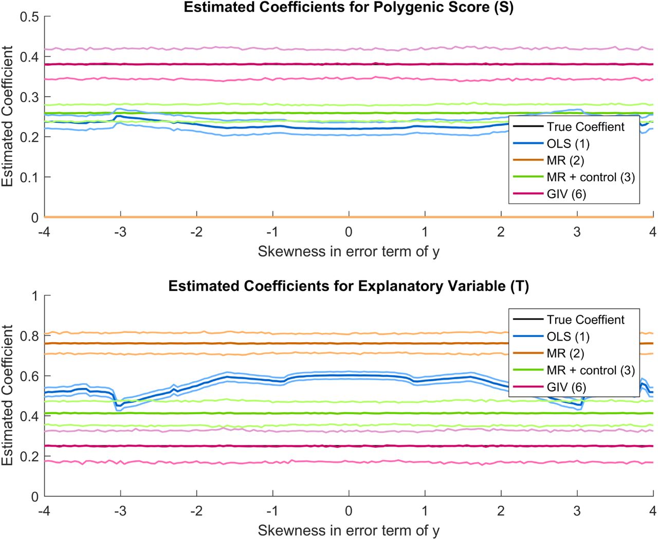
Model with measurement errors and skewness in y
Estimated coefficients for model A, using various methods. The mean of the simulations for each method is shown, together with simulated 95% confidence interval is shown. The simulations are based on a sample of 8,600, assuming 300,000 independent SNPs, a heritability of 0.2 and 0.55 for y and T respectively, a genetic correlation of 0.15, a coefficient of 0.15 for effect of T on y and a correlation of 0.4 between the error terms in y and T. The total GWAS sample size is 1,000,000. Skewness is added to the error term in y.

Model with measurement errors and kurtosis
Estimated coefficients for model A, using various methods. The mean of the simulations for each method is shown, together with simulated 95% confidence interval is shown. The simulations are based on a sample of 8,600, assuming 300,000 independent SNPs, a heritability of 0.2 and 0.55 for y and T respectively, a genetic correlation of 0.15, a coefficient of 0.15 for effect of T on y and a correlation of 0.4 between the error terms in y and T. The total GWAS sample size is 1,000,000. Kurtosis is added to the error term in y and T.

Model with dependent measurement errors between multiple indicators of S
Estimated coefficients for model A, using various methods. The mean of the simulations for each method is shown, together with simulated 95% confidence interval is shown. The simulations are based on a sample of 8,600, assuming 300,000 independent SNPs, a heritability of 0.2 and 0.55 for y and T respectively, a genetic correlation of 0.15, a coefficient of 0.15 for effect of T on y and a correlation of 0.4 between the error terms in y and T. The total GWAS sample size was 1,000,000. The measurement errors in the PGS for y are correlated, the one in PGS for T is independent.

Model with dependent measurement errors among T and multiple indicators of S (all correlations assumed equally large)
Estimated coefficients for model A, using various methods. The mean of the simulations for each method is shown, together with simulated 95% confidence interval is shown. The simulations are based on a sample of 8,600, assuming 300,000 independent SNPs, a heritability of 0.2 and 0.55 for y and T respectively, a genetic correlation of 0.15, a coefficient of 0.15 for effect of T on y and a correlation of 0.4 between the error terms in y and T. The total GWAS sample size was 1,000,000. The measurement errors in all PGS are correlated.

Model with correlations between common and rare genetic variances
Estimated coefficients for model A, using various methods. The mean of the simulations for each method is shown, together with simulated 95% confidence interval is shown. The simulations are based on a sample of 8,600, assuming 300,000 independent SNPs, a heritability of 0.2 and 0.55 for y and T respectively, a genetic correlation of 0.15, a coefficient of 0.15 for effect of T on y and a correlation of 0.4 between the error terms in y and T. The total GWAS sample size was 1,000,000. Unobserved causal genetic variants were added too model A.

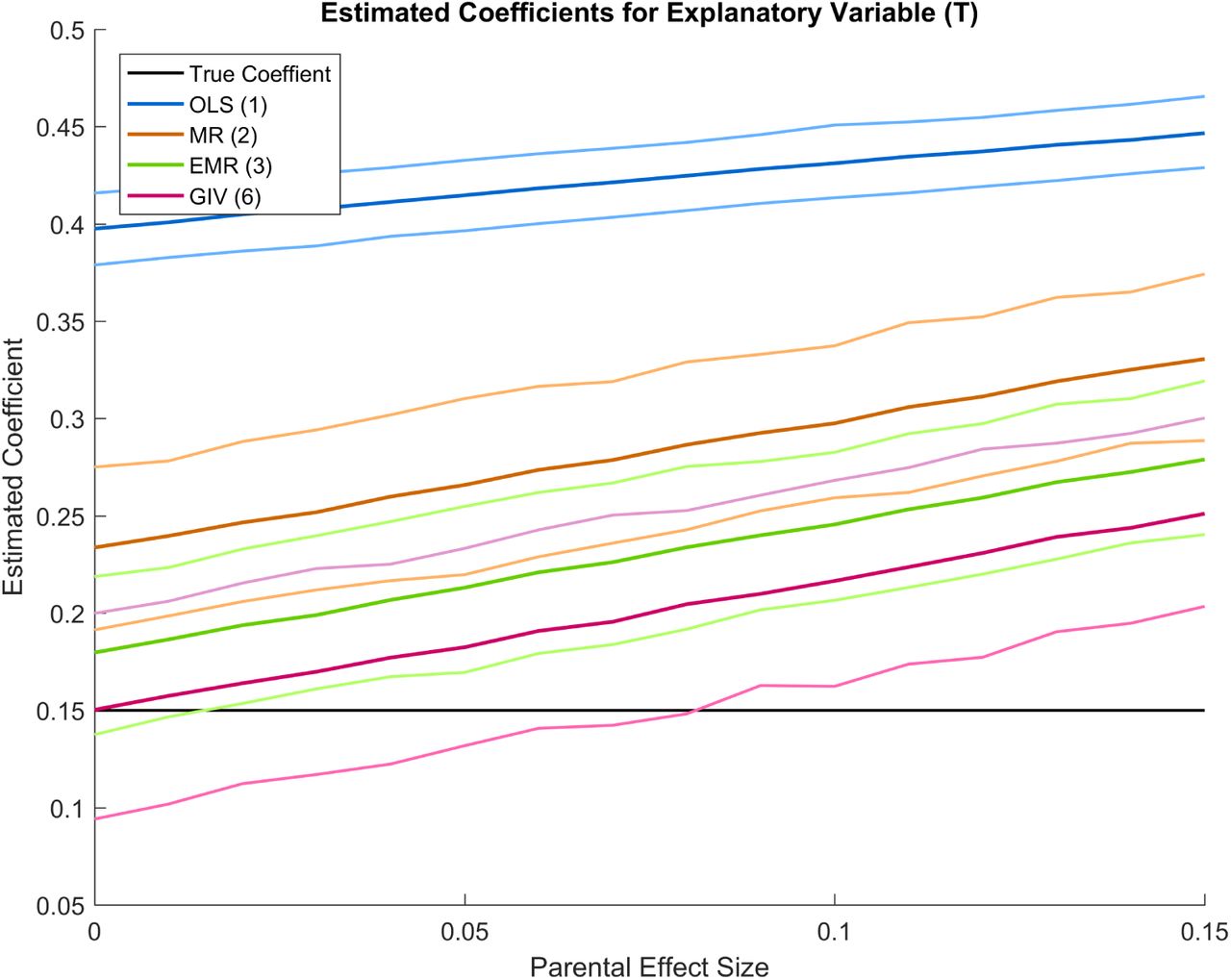
Model with parental effects
Estimated coefficients for model A, using various methods. The mean of the simulations for each method is shown, together with simulated 95% confidence interval is shown. The simulations are based on a sample of 8,600, assuming 300,000 independent SNPs, a heritability of 0.2 and 0.55 for y and T respectively, a genetic correlation of 0.15, a coefficient of 0.15 for effect of T on y and a correlation of 0.4 between the error terms in y and T. The total GWAS sample size was 1,000,000. Unobserved parental effects were added to model A.
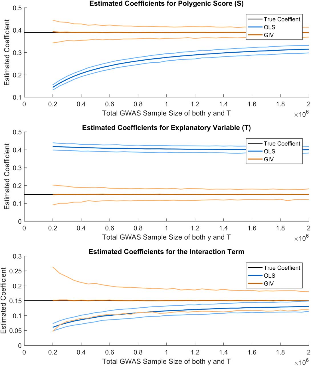
Model with interaction term
Estimated coefficients for model B, using OLS and GIV. The mean of the simulations for each method is shown, together with simulated 95% confidence interval is shown. The simulations are based on a sample of 8,600, assuming 300,000 independent SNPs, a heritability of 0.2 and 0.55 for y and T respectively, a genetic correlation of 0.15, a coefficient of 0.15 for effect of T on y, a coefficient of 0.15 for the interaction term and a correlation of 0.4 between the error terms in y and T. The total GWAS sample size was 1,000,000. Unobserved parental effects were added to model A.
Simulations
We explored the robustness of GIV regression in finite sample sizes using a range of simulation scenarios (SI appendix). The simulations generate data from a set of known models, which we then analyzed to produce coefficient estimates of the effect of the PGS for y on y and the effect of T on y. We produce these estimates using OLS, MR, EMR, and GIV regression, and compare these results with the true answer across a range of parameter values. The simulations specify that the true PGS scores for y and T are correlated and that the observed PGS scores for y and T are constructed with error. We make the conservative assumption that the entire genetic correlation between the traits is due to Type 1 pleiotropy, all genes that are associated with both phenotypes have direct effects on both.5 In practice, this is unlikely to be the case, but it is equally unlikely that one can put a credible upper bound on (or completely rule out) Type 1 pleiotropy. In one set of scenarios, we make the assumption that the entire endogeneity problem arises from the genetic correlation between y and T, a problem which would be solved if we could measure the PGS for these two phenotypes without error. In a second set of simulations, we make the additional assumption that endogeneity arises from other (e.g., environmental) sources that cause the disturbance term in the structural equation for y to be correlated with the disturbance term in the structural model for T even if the true PGS for y and for T were in the respective structural equations. In a third set of simulations, we assume that the genetic factors that affect T are correlated with the environmental factors in the disturbance term for y, as would be the case if parental genes, which affect the PGS for T, also either cause or select for environmental factors that affect y net of T and the PGS for y. We conducted simulations which alternatively specify that the effects of T and the PGS for y are additive and that the effects interact (i.e., where the effect of T on y depend on the PGS for y). The simulations alternately assume that the underlying distributions for the errors in the structural equations for y and T are multivariate normal and deviate from normal via the introduction of skew and kurtosis. They also alternately assume that the errors in the equation for the observed PGS for T and the multiple observed PGS for y are independent or correlated. Finally, we simulate the scenario where even the true PGS for y and T fail to capture all the genetic effects on y and T because they omit rare genetic variants, and where the rare variants for y are correlated with the rare variants for T.
The details of these simulation results are described in the SI appendix. The results provide considerable support for the claim that GIV regression greatly improves our ability to estimate the effects of variables that may have a causal effect on an outcome variable but where genetic correlation and other forms of endogeneity are present. When the only problem is measurement error in the PGS for y and T, GIV regression produces results that bracket the true answer. GIV regression also provides accurate results when the errors of the two structural models are correlated for reasons beyond measurement error in the PGS. Skewness and Kurtosis in the distributions of the errors do not much affect the quality of GIV regression estimates.
When the measurement errors of the PGS are correlated (i.e. when overlapping GWAS samples were used to construct the PGS for y and the genetic IVs), the exclusion restriction is violated and GIV regression estimates are biased. However, we find that GIV regression still outperforms MR or EMR for small to moderately correlated measurement errors (ρ < 0.5). It is also encouraging to find that missing genetic variants from the PGS for y and T do not lead to noteworthy bias in the GIV regression estimate for the effect of T on y. Finally, we find that in situations where endogeneity is induced by the effects of or correlation between parental genes and the environment of the parent’s children, estimates from all methods are, as expected, biased. However, we still find that GIV regression outperforms all other methods in terms of the size of the bias of the estimated effect of T on the outcome. In the next section, we discuss these scenarios and our results in greater detail.
Violated assumptions
We now elaborate on the assumptions that GIV regression is based on, and discuss what our simulations tell us about how GIV regression performs under potential violations in comparison with OLS, MR, and EMR.
1. Complete genetic information: Current GWAS are based on two technologies to obtain genetic data. First, so-called genotyping arrays are used to extract information from DNA samples for a selected sub-set of genetic markers. Array technologies allow high throughput and are substantially cheaper than sequencing the entire human genome, which mostly consists of genetic information that does not vary among humans. Instead, array technologies focus on genetic markers that are known to vary within or across specific human populations. Second, one makes use of the fact that genetic markers which are physically close to each other on a chromosome tend to be correlated. This allows genotyping arrays to focus on one or a few SNPs per region that represent the genetic variations (so-called haplotypes) which can be found among humans. Next, information from fully sequenced reference samples is used to impute the missing SNPs [49]. This approach yields highly accurate information for common genetic polymorphisms [50]. However, genotyping and imputation accuracy attenuate strongly for rare polymorphisms as well as for so-called structural genetic variants (e.g. deletions, insertions, inversions, copy-number variants) that are not directly included in the genotyping array. Newer genotyping arrays tend to capture more and better selected polymorphisms than older arrays. Furthermore, increasing sample sizes of completely sequenced reference populations allow imputation of missing genetic variants with ever increasing accuracy [50]. Nevertheless, this implies that the assumption of complete genetic information is violated in practice, although this is likely to be a temporary issue. Another implication of this assumption is that it will be important in practice to ensure that all PGS used in GIV regression are constructed from the same or at least from largely overlapping sets of SNPs.6
While it is not possible to know the impact of genetic variants that are not yet included in GWAS data, recent research [47] finds that the 1000 Genomes imputed data imply very little bias for our method arising from correlation between missing genetic information and the SNPs used to estimate the PGS for height, because the 1000 Genomes imputed data contains almost all the narrow-sense heritability of these traits. Specifically, we used Yang et al’s results to infer the effects of rare variants on y (and also on T) in the SI appendix, and we then computed the bias via simulations using a range of correlations between common and rare genetic variants. The simulation shows that our results are robust across a range of plausible values for these correlations (Supplementary Figure 12).
2. Genetic effects are linear: Possible violations of this assumption could arise if non-linear genetic effects such as systematic gene-gene interactions (a.k.a. epistasis) ended up in the error terms of both scores or if y is affected by genetic dominance or by unmeasured genetic markers (e.g. very rare alleles or structural variants not included in the GWAS or the prediction sample). In other words, suppose that the true structural equation is
 where f (G) includes interaction terms between the various genetic markers in G, the effects of unmeasured genetic markers and other nonlinear effects. The presence of f (G) in equation (5) may cause the exclusion rule to be violated; Sy2 may be correlated with the disturbance term because
  may be correlated with the non-zero interaction effects in f (G). This problem is not solved even if the measurement error in the PGS was essentially eliminated through the use of extremely large GWAS samples and using ordinary least squares to estimate equation (5); the problem stems from the failure to control for (or find an instrument for) f (G). Imagine that
  perfectly captures the linear effects of the measured SNPs. If f (G) is uncorrelated with
  , then the estimated effect of
  will be consistent, but the estimate of the proportion of variance in y that is statistically explained by genetic factors will be underestimated and the standard error of the effect of
  will be higher than if f (G) were observed. If f (G) is positively correlated with
  , then the true effect of
  will be overestimated and the total variance explained by genetic factors will be underestimated. If f (G) is negatively correlated with
  , then the true effect of
  will be underestimated and the total variance explained by genetic factors will also be underestimated. Epistasis certainly exists to some extent. However, the observed twin correlations for the majority of traits (69%) are consistent with a simple and parsimonious model where twin resemblance is solely due to additive genetic variation and where epistasis is therefore not a major problem [8].
3. Genome-wide association studies successfully control for population structure: Violations of this assumption lead to biased PGS or to PGS that predict y for non-genetic reasons (as when a model without population controls makes it seem as if Italians like pasta or the Chinese use chopsticks for genetic reasons) [20]. This can lead to the violation of the exclusion restriction if the population structure variables that are correlated with  are not controlled for in the PGS or the structural model, and if these population variables affect the outcome of interest. Multiple indicators of
  would not resolve this omitted variable bias because each of these indicators would also be correlated with the omitted variables.
4. It is possible to divide GWAS samples into non-overlapping sub-samples drawn from the same population as the sample used for analysis. In principle, this assumption seems unproblematic: the availability of large-scale, population-based, genotyped datasets such as the UK Biobank makes it straightforward to randomly split the sample into parts and to exclude genetically related or identical observations. One practical issue is that one may want to use results from published GWAS studies to construct polygenic scores. In this case, it should be verified that the genetic architecture of the trait is identical in the GWAS results and the analysis sample (e.g. using bivariate LD score regression [12]). Furthermore, most GWAS studies are conducted as a meta-analysis of summary statistics from various samples. Metaanalysis circumvents legal, practical, and logistic challenges that would have to be overcome to pool data from several providers on one central location is as statistically powerful as analyzing the raw data directly [51]. However, the meta-analysis approach makes it difficult to check if the same or closely related individuals have been included in several samples. It is currently unknown if and to which extent such hidden overlap between GWAS samples is a real issue. We explore in SI section 3.2.2 the consequences of a correlation between the measurement errors of the polygenic scores. As can be seen from Supplementary Figures 10 and 11, when the measurement errors for Sy1 and Sy2 are not independent, all methods produce biased estimates. When the correlation between the measurement errors of the PGS for y is small, GIV regression outperforms the other methods. When the correlation becomes moderate to strong, none of the methods produce accurate estimates. When the measurement errors in Sy1 and Sy2 are correlated with the measurement error in T, there is a region of small to moderate correlation strength in which EMR performs better than GIV regression or MR. When the correlation is strong, none of the methods produce accurate estimates.
5. The PGS for the outcome is uncorrelated with omitted inherited environmental factors that affect the outcome. An example of potential bias stemming from omitted inherited environmental factors would arise from the correlation between the PGS for height and the PGS for parent’s height, which is correlated with parent’s height, under conditions when parents get an environmental effect from height (e.g., higher pay for being taller) that affects the quality of the childhood health environment that could be correlated both with child’s height and with child’s EA. Violation of the exclusion restriction would be avoided by controlling for parental height, or for the parental resources that are consequences of parental height. More generally, however, there might be other causal pathways between parental genetic factors that affect the child’s environment in ways that affect her EA (e.g., via the BMI of parents). One alternative strategy for blocking these pathways would be to construct and control for a parental PGS for the child’s EA. However, large family samples including biological parents and their offspring would be required for this. Such samples are still very rare and often not available in the public domain. Furthermore, in the absence of sufficiently large GWAS samples to estimate parental PGS with high accuracy, controlling for the observed parental PGSs would not be perfect, for the same reasons described throughout this paper in the context of a person’s own PGS (though it would then in principle be possible to pursue a multiple indicator strategy for parental PGS as we do for the child’s PGS). Whether it would be preferable to control for the parental PGS (and to use an additional indicator of the PGS to obtain consistent estimates of the effect of the parental PGS on the outcome) or for parental phenotypical characteristics that might affect a person’s life course environment, or for the environmental characteristics themselves would depend upon whether the causal pathways are well-enough understood and whether sufficient information is available about a person’s environment, her parent’s phenotypical characteristics, or her parent’s PGS for the person’s outcome of interest in the analysis.
To assess the potential impact of bias from omitted inherited environmental factors that are correlated with the IVs, we carried out a final simulation where we assumed that a genetic marker of the parents (PT) affects y net of  and T. We assumed a range of values for the effect of PT allowing its effect to range from zero to the same size as T in our structural model (equation 3). Supplementary Figure 13 shows that GIV regression generally outperforms OLS, MR, and EMR, but that all methods produce sub-stantial bias if the reduced form effect of PT, which affects y entirely indirectly through omitted environmental factors, rivals the effect of T on y. In practice, the problem is unlikely to be this large; even if the indirect effects of parental genes through their effect on the child’s environment are sizable, much of the bias can be removed from the estimation via controls for these consequential environmental variables or for the parental phenotypical characteristics that produce these environmental effects (e.g., parental education or income or height), or for the parental genotype (via a PGS for the genetic effects of parents on or through the use of data on twins that allows an effective control of parental genotype via the estimation of within-family regression models.
Empirical applications
We illustrate the practical use of GIV regression in a variety of important empirical applications using data from the Health and Retirement Survey (HRS) for 8,638 unrelated individuals of North-West European descent who were born between 1935 and 1945 (SI appendix).
The narrow-sense SNP heritability of educational attainment
First, we estimate the chip heritability of EA using GIV regression (see SI appendix).
The results are displayed in Table 1. The standard OLS estimate of the PGS only explains 4% of the variance in EA, which is similar to the results reported by the Social Science Genetic Association Consortium [27]. This is substantially lower than the 17.3% estimate of chip heritability (with a 95% confidence interval of +/- 4%) reported by [52] in the same data using genomic-relatedness-matrix restricted maximum likelihood (GREML).7 Columns 2 and 3 show GIV regression results using one or the other of the two subset PGS scores as the covariate and as the instrumental variable. The 2SLS regression in column 2 gives an estimate of.364, while the 2SLS regression in column 3 gives an estimate of.454. These estimates imply 13% and 21% respectively as the estimates of SNP-based heritability, and so confidence intervals around these point estimates are consistent with the GREML estimate from [52]. In other words, GIV regression recovers the correct chip heritability from polygenic scores.8
Effects of the PGS on Educational Attainment in the HRS subsample
The relationship between body height and educational attainment
Previous studies using both OLS and sibling or twin fixed effects methods have found that taller people generally have higher levels of EA [53, 54, 55]. They are also more likely to perform well in various other life domains, including earnings, higher marriage rates for men (though with higher probabilities of divorce), and higher fertility [56, 57, 58, 59, 60, ?]. The question is what drives these results. Can they be attributed to genetic effects that jointly influence these outcomes? Are there social mechanisms that systematically favor taller or penalize shorter individuals? Or are there non-genetic factors (e.g., the uterine and post-birth environments especially related to nutrition or disease) that affect both height and these life course outcomes? The literature on the relationship between height and EA has found evidence that the association arises largely through the relationship between height and cognitive ability, which may suggest that the height-EA association is driven largely by genetic association between height and cognitive ability. We use GIV regression with individual-level data from the HRS to clarify the influence of height on EA, and we compare these results with those obtained from OLS and from MR. In addition, we conduct a “negative control” experiment that estimates the causal effect of EA on body height (which should be zero). A complete description of the materials and methods is available in the SI Appendix.
GWAS summary statistics for height were obtained from the Genetic Investigation of ANthropo-metric Traits (GIANT) consortium [22] and by running a GWAS on height using the interim release of genetic data in the UK Biobank [61], which was not part of the GIANT sample. We refer to these as Height_GIANT and Height_UKB, respectively. GWAS summary statistics for EA were obtained from the Social Science Genetic Association Consortium (SSGAC). The most recent study of the SSGAC on EA used a meta-analysis of 64 cohorts for genetic discovery and the interim release of the UKB for replication [27]. We refer to these samples as EA_SSGAC and EA_UKB, respectively. There is an overlap in the cohorts between Height_GIANT and EA_SSGAC. To ensure independence of measurement errors in the PGS, whenever one of the two was used as regressor, we excluded the other as instrument and used a PGS from UK Biobank data instead.
The OLS results in Table 2 show that height (in meters) appears to have a strong effect on years of EA, with two additional centimeters in height generating one additional month of EA. MR appears to confirm the causal interpretation of the OLS result; indeed, the point estimate from MR is even slightly larger than from OLS. As discussed above, MR suffers from probable violations of the exclusion restriction. These violations could stem from the possibility that the some genes have direct effects on both height and EA (i.e. Type 1 pleiotropy).9 They could also stem from the possibility that the PGS for height by itself is correlated with the genetic tendency for parents to have higher EA and income, and therefore a lower nutritional or disease risk for their children, who therefore are more likely to reach their full cognitive potential and have higher EA. Controlling for the PGS is an imperfect strategy for eliminating this source of endogeneity, because the bias in the estimated effect of the PGS score also biases the estimated effect of height (the omitted variable bias discussed earlier).
Regression of educational attainment on height in the Health and Retirement Study (HRS)
In contrast, estimates from GIV regression in Table 2 show both a considerably larger effect of the education PGS score on EA, and a small and statistically insignificant effect of height on EA. These results imply that the positive correlation between height and EA is not a causal relationship. Rather, the observed phenotypic correlation is primarily due to the genetic correlation between the two traits. Furthermore, our “negative control” using GIV regression finds no causal effect of EA on height, as expected. One might contrast our results also to those of [53], who found a correlation between the height and EA of Finnish monozygotic (MZ) twins. Silventoinen et al’s study effectively controls for all genetic correlation between height and EA. However, their result would still suffer from endogeneity bias to the extent that the difference in MZ twin heights is related to intra-uterine or post-birth environmental differences that cause one twin to be taller and have higher cognitive or non-cognitive abilities than the other twin. GIV regression is arguably superior to twins fixed effects to the extent that these environmental variables are uncorrelated with the PGS for height once the PGS for EA is effectively controlled, making the combination of the PGS for height and the PGS for EA to be valid instruments.
Conclusion
Accurate estimation of causal relationships with observational data is one of the biggest and most important challenges in epidemiology and the social sciences -two fields of inquiry where many questions of interest cannot be adequately addressed with properly designed experiments due to practical or ethical constraints. Here, we have proposed a method that allows genetic data to be used for this purpose. Thinking of genetic data as a sort of naturally occurring experiment is appealing because the genotypes that arise from two mates are randomized by the process of meiosis. Thus, given that virtually all human traits are heritable to some extent, an individual’s genotype could in principle be used to identify causal effects across a wide range of important scientific questions. Thanks to cheap and accurate genotyping technologies and growing insights into the genetic architecture of many traits via large-scale GWAS, this general idea becomes practically more and more feasible. In principle, it is this idea which underlies so-called Mendelian Randomization (MR)–a method suggested by epidemiologists that uses genetic data as instrumental variables.
The crucial identifying assumption of MR is that the genes which are used as instruments do not also affect the outcome through other causal pathways via so-called pleiotropic effects. In light of the widespread and often substantial genetic correlations between many traits, this assumption seems problematic. We have proposed a new strategy that we call genetic instrumental variable (GIV) regression, that eliminates or at least substantially reduces the bias of MR due to pleiotropy under a set of arguably more realistic assumptions. We have explored conditions where the assumptions underlying GIV regression will fail and conclude that GIV regression outperforms OLS and MR in a broad range of realistic scenarios.
The simulations described in the paper certainly do not cover all conceivable data generating processes, but they are nonetheless of considerable utility, we would argue, in assessing the performance of GIV regression. Analyses with real data demonstrate that GIV regression recovers estimates of the effect size of the outcome PGS that are consistent with alternative approaches to estimate the extent of narrow-sense heritability. Our analyses also provide reason to be cautious when using OLS or MR to estimate causal effects between variables that are known to be genetically correlated. Existing knowledge about the effects of epistasis, rare or dominant alleles, structural variants, or population structure provide good grounds to be cautiously optimistic that GIV regression provides an important tool for assessing causal effects when unmeasured genetic correlation is likely to be a serious issue. In particular, constant improvements in genotyping technology, increasing GWAS samples, and even better statistical methods to control for population structure in GWAS will make it less and less likely in the future that the assumptions underlying our approach will be seriously violated. Additional knowledge in this rapidly developing field will provide further guidance for assessing the extent of remaining bias in GIV regression estimates. The combination of new estimation tools and continued rapid advancements in genetics should provide a significant improvement in our understanding of the effects of behavioral and environmental variables on important socioeconomic and medical outcomes.
Supplementary Tables
Cohort list for Educational Attainment
Cohort list for Height
Regression of height on educational attainment in the Health and Retirement Study (HRS)
References
- [1].↵
- [2].↵
- [3].↵
- [4].↵
- [5].↵
- [6].↵
- [7].↵
- [8].↵
- [9].↵
- [10].↵
- [11].↵
- [12].↵
- [13].↵
- [14].↵
- [15].↵
- [16].↵
- [17].↵
- [18].↵
- [19].↵
- [20].↵
- [21].↵
- [22].↵
- [23].↵
- [24].↵
- [25].↵
- [26].↵
- [27].↵
- [28].↵
- [29].↵
- [30].↵
- [31].↵
- [32].↵
- [33].↵
- [34].↵
- [35].↵
- [36].↵
- [37].↵
- [38].↵
- [39].↵
- [40].↵
- [41].↵
- [42].↵
- [43].↵
- [44].↵
- [45].
- [46].↵
- [47].↵
- [48].↵
- [49].↵
- [50].↵
- [51].↵
- [52].↵
- [53].↵
- [54].↵
- [55].↵
- [56].↵
- [57].↵
- [58].↵
- [59].↵
- [60].↵
- [61].↵
References
- [1].
- [2].
- [3].
- [4].
- [5].
- [6].
- [7].
- [8].
- [9].
- [10].
- [11].
- [12].
- [13].
- [14].
- [15].
- [16].
- [17].
- [18].
- [19].
- [20].
- [21].
- [22].
- [23].
- [24].
- [25].
- [26].
- [27].
- [28].
- [29].
- [30].
- [31].
- [32].
- [33].
- [34].
- [35].
- [36].
- [37].
- [38].
- [39].
- [40].
- [41].
- [42].


