

Abstract
Single-cell RNA-seq (scRNA-seq) is widely used to investigate the composition of complex tissues1–9 since the technology allows researchers to define cell-types using unsupervised clustering of the transcriptome8,10. However, due to differences in experimental methods and computational analyses, it is often challenging to directly compare the cells identified in two different experiments. Here, we present scmap, a method (source code available at https://github.com/hemberg-lab/scmap and the application can be run from http://www.hemberg-lab.cloud/scmap) for projecting cells from a scRNA-seq experiment on to the cell-types identified in a different experiment.
Main text
As more and more scRNA-seq datasets become available, carrying out comparisons between them is key. Such comparisons will be of particular importance once there are well-annotated references available, e.g. the Human Cell Atlas (HCA)11. One of the key applications will be to project cells from a new sample (e.g. from a disease tissue) onto the reference to characterize differences in composition or to detect new cell-types. Conceptually, such projections are similar to the popular blast12 method, which makes it possible to quickly find the closest match in a database for a newly identified nucleotide or amino acid sequence.
Projecting a new cell, c, onto a reference dataset that has previously been grouped into clusters, amounts to identifying which cluster c is most similar to. We represent each cluster by its centroid, i.e. a vector of the median value of the expression of each gene, and we measure the similarity using a suitable distance metric. Instead of using all genes when calculating the similarity, we use unsupervised feature selection to include only the genes that are most relevant for the underlying biological differences which allows us to overcome batch effects13.
We investigate three different strategies for feature selection: random selection, highly variable genes (HVGs)14 and genes with a higher number of dropouts than expected (M3Drop)13. To increase speed, we modified the M3Drop method and instead of fitting a Michaelis-Menten model to the log expression-dropout relation, we fit a linear model (Methods, Fig. 1a). For the number of features, we used the top 10, 100, 200, 500, 1000, 2000, 5000, or all genes. Similarities were calculated using the cosine, Pearson and Spearman distances. These distances metrics are all restricted to the interval [-1, 1], which means that they are insensitive to differences in scale between datasets. To make the assignments more robust, we required that at least two of the three similarity measures were in agreement and that the similarity exceeded.7 for at least one of the measures. If these criteria are not met, then the cell is labelled as “unassigned” to indicate that it does not correspond to any cell-type present in the reference.
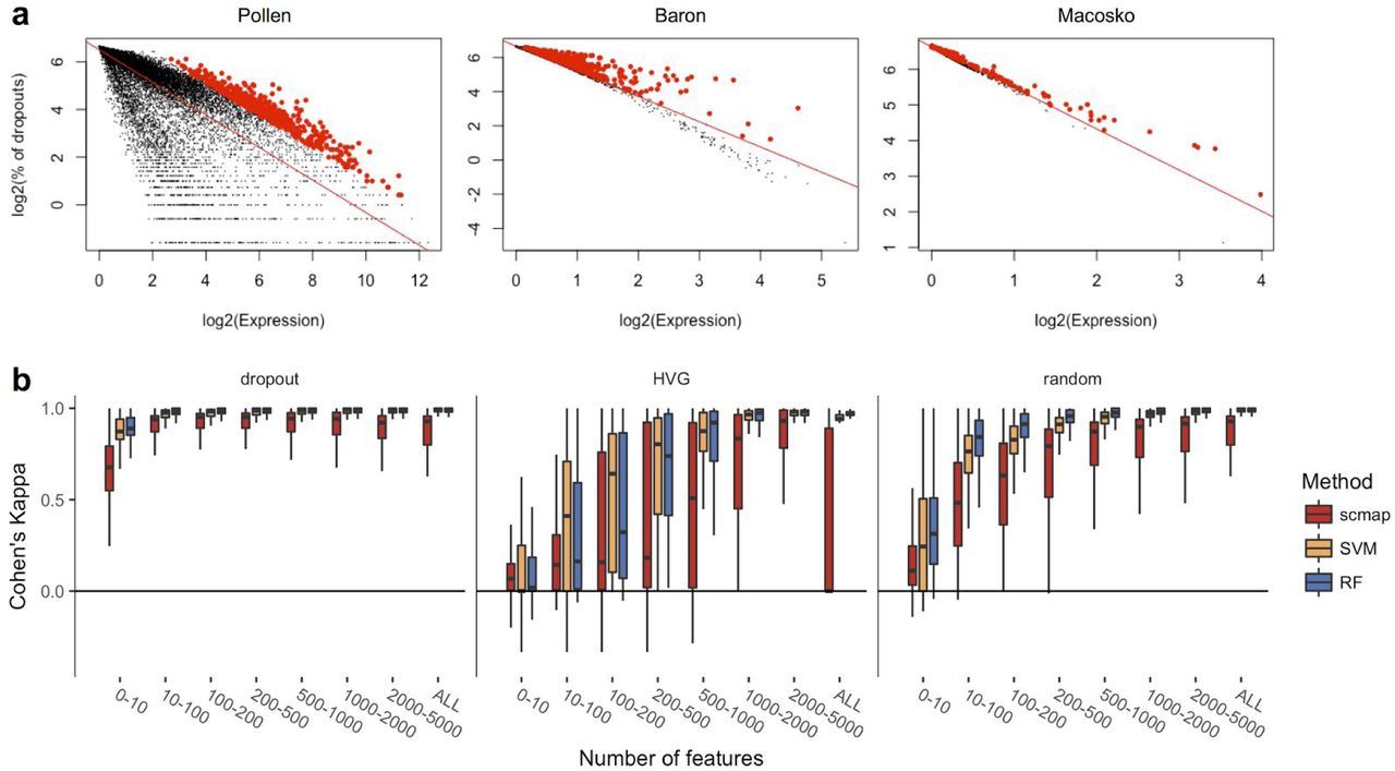
(a) Dropout-based feature selection (see Methods) for Pollen15 (SMARTer protocol), Baron4 (inDrop16 protocol) and Macosko8 (Drop-seq8 protocol) datasets. Red line represents a linear fit to the distribution of the points, red points represent top 500 positive residuals of the fit. (b) Cohen’s κ values of self-projections, corresponding to dropout-based, HVG14 and random feature selections. The plot is based on 16 datasets1–9,15–21. For each dataset 70% of all cells are sampled 100 times and the rest 30% of cells are projected to it.
To validate the projections, we considered 16 different datasets1–9,15–21 from mouse and human, collected and processed in different ways. We first carried out a self-projection experiment where each dataset is mapped onto itself. We used 70% of the cells from the original sample for the reference and the remaining 30% are projected, with clusters as defined by the original authors. To quantify the accuracy of the mapping, we use Cohen’s K22 which is an index that is suitably normalized to account for the sizes of the groups. A value of 1 indicates that the cluster assignment was in complete agreement with the original labels, whereas 0 indicates that the assignment is no better than random guessing. We find that the dropout-based method for feature selection has the best performance, and somewhat surprisingly we also find that random selection is better than HVG (Fig. 1b). We also note that the dropout-based method is robust when the number of features are selected in the range 100 to 1000. As a comparison, we also considered two supervised methods for projecting new samples, a random forests classifier (RF) and a support vector machine (SVM). These classifiers were trained on the reference and then used on the held out parts as before. For both RF and SVM we find that the performance is slightly better than scmap for all three feature selection methods.
As a positive control, we considered seven pairs of datasets (Table S1) that we expect to correspond well based on their origin. The results showed that scmap outperforms RF and SVM, and that scmap consistently obtains K>.75 when the number of features used was between 100 and 1,000 (Fig. 2a). Even though RF performs significantly better than scmap and SVM in this range, the higher κ can be explained by the fact that the RFs have a much higher fraction of unassigned cells (Fig. 2b). An important aspect of the positive control experiments is that for 6 of the pairs, one of the datasets was collected using a full-length protocol and the other was collected using a UMI based protocol. Despite the substantial differences between the protocols16,23,24, scmap has no problems comparing the datasets.

(a) Cohen’s κ values and (b) percentage of unassigned cells for positive controls. The plots are based on 7 pairs of datasets listed in Table S1 (projections are performed in both directions). Dropout-based feature selection is used everywhere (see Methods).
As a negative control, we projected datasets with an altogether different origin from the reference (e.g. mouse retina onto mouse pancreas, Table S2). Reassuringly, we found that the dropout based strategy categorized >90% of the cells as unassigned when the number of features used was greater than 200 (Fig. 3). Notably, SVM has a much smaller fraction of unassigned cells than RFRef16 and scmap. Taken together, comparing the evidence across the self-projection experiments, the positive and negative controls, we conclude that scmap with 500 features provides the best performance balancing K and fraction of unassigned cells.

Percentage of unassigned cells in negative controls. The plot is based on 10 pairs of datasets listed in Table S2 (projections are performed in both directions). Dropout-based feature selection is used everywhere (see Methods).
An important feature of scmap is that it is very fast, using 1,000 features it takes only around twenty seconds to map 40,000 cells, compared to almost thirty minutes using RF or SVM (Fig. 4). Since the complexity scales with the number of clusters in the reference, rather than the number of cells, scmap will be applicable to large scale datasets. Moreover, the run-time can be further improved since the centroids and features for each cluster can be pre-computed, and stored in memory, even for a very large atlas.

CPU run times of scmap, SVM and RF. The x-axis represents a number of cells in the reference dataset. For all methods 1,000 features and 10,000 cells in the projection dataset were used. All methods were run on a MacBook Pro laptop (Mid 2014), OS X Yosemite 10.10.5 with 2.8 GHz Intel Core i7 processor, 16 GB 1600 MHz DDR3 of RAM. Points are actual data, solid lines are “loess” fit to the points with span = 1 (see ggplot2 documentation). Dashed lines are manual linear extrapolation of the solid lines.
We have implemented scmap as an R-package and it will be submitted to Bioconductor to facilitate incorporation into bioinformatic workflows and the fact that scmap is scater-based25, makes it easy to combine with other computational scRNA-seq methods. Moreover, we have made scmap available via the web, allowing users to either upload their own reference or to use one of the datasets from this paper. For the website, we also provide pre-calculated feature selections and centroids for the 16 datasets used in this study to speed up the projections.
One of the main challenges in analyzing scRNA-seq datasets is to provide biological interpretations and annotations of the identified clusters. By comparing to existing, previously annotated datasets, this part of the analysis will be sped up. Much like blast for nucleotides, scmap will facilitate fast and accurate comparisons of newly found cells to an established reference. Moreover, a robust, fast and accurate method for comparing populations identified from different experiments will be a crucial component of the HCA and similar efforts to build scRNA-seq references as it will facilitate quality control and help ensure consistency across experimental samples.
Methods
Datasets
All datasets and cell type annotations were downloaded from their public accessions. All datasets were converted into scater25 objects. Details of the scater objects creation are available on our dataset website (https://hemberg-lab.github.io/scRNA.seq.datasets). In some datasets similar cell types were merged, namely:
In Deng17 dataset zygote and early2cell were merged into zygote cell type, mid2cell and late2cell were merged into 2cell cell type, and earlyblast, midblast and lateblast were merged into blast cell type.
All bipolar cell types of the Shekhar9 dataset were merged into bipolar cell type.
In Yan19 dataset oocyte and zygote cell types were merged into zygote cell type.
Feature selection
To select informative features we used a method conceptually similar to M3Drop13 to relate the mean expression (E) and the dropout rate (D). Instead of modelling the relation between log(E) and D using Michaelis-Menten kinetics, we used a linear model to capture the relationship log(E) and log(D). After fitting a linear model using the lm() command in R, important features were selected as the top N residuals of the linear model (Fig. 1a). The feature selection is calculated for the reference only, and those genes absent or zero in the projection set are not used.
Reference centroid
Each cell type in the reference dataset is represented by its centroid, i.e. the median value of gene expression across all cells in that cell type.
Projection dataset
Projection of a dataset to a reference dataset is performed by calculating similarities between each cell and all centroids of the reference dataset, using only the selected features. Three similarity measures are used: Pearson, Spearman and Cosine. The cell is then assigned to the cell type which correspond to the highest similarity value. However, scmap requires that at least two similarity measures agree with each other, otherwise the cell is marked as “unassigned”. Additionally, if the maximum similarity value across all three similarities is below a similarity threshold (default is .7), then the cell is also marked as “unassigned”. Positive and negative control plots corresponding to Figs. 2 and 3 for different values of the similarity/probability (see SVM and RF) threshold (.5, .6, .8 and .9) are shown in Figs. S1-S3
SVM and RF
scmap projection algorithm was benchmarked against support vector machines26 and random forests27 classifiers from the R packages e1071 and randomForest. The classifiers were trained on all cells of the reference dataset and a cell type of each cell in the projection dataset was predicted by the classifiers. Additionally, a threshold (default value of .7) was applied on the probabilities of assignment: if the probability was less than the threshold the cell was marked as “unassigned”.
Conflicts of interest
None.
Acknowledgements
We would like to thank Tallulah Andrews, Guillermo Parada, and Florian Wünnermann for helpful discussions and feedback on the manuscript and for testing the cloud implementation of scmap.


