Bayesian Efficient Coding

Abstract

The efficient coding hypothesis, which proposes that neurons are optimized to maximize information about the environment, has provided a guiding theoretical framework for sensory and systems neuroscience. More recently, a theory known as the Bayesian Brain hypothesis has focused on the brain’s ability to integrate sensory and prior sources of information in order to perform Bayesian inference. However, there is as yet no comprehensive theory connecting these two theoretical frameworks. We bridge this gap by formalizing a Bayesian theory of efficient coding. We define Bayesian efficient codes in terms of four basic ingredients: (1) a stimulus prior distribution; (2) an encoding model; (3) a capacity constraint, specifying a neural resource limit; and (4) a loss function, quantifying the desirability or undesirability of various posterior distributions. Classic efficient codes can be seen as a special case in which the loss function is the posterior entropy, leading to a code that maximizes mutual information, but alternate loss functions give solutions that differ dramatically from information-maximizing codes. In particular, we show that decorrelation of sensory inputs, which is optimal under classic efficient codes in low-noise settings, can be disadvantageous for loss functions that penalize large errors. Bayesian efficient coding therefore enlarges the family of normatively optimal codes and provides a more general framework for understanding the design principles of sensory systems. We examine Bayesian efficient codes for linear receptive fields and nonlinear input-output functions, and show that our theory invites reinterpretation of Laughlin’s seminal analysis of efficient coding in the blowfly visual system.

One of the primary goals of theoretical neuroscience is to understand the functional organization of neurons in the early sensory pathways and the principles governing them. Why do sensory neurons amplify some signals and filter out others? What can explain the particular configurations and types of neurons found in early sensory system? What general principles can explain the solutions evolution has selected for extracting signals from the sensory environment?

Two of the most influential theories for addressing these questions are the “efficient coding” hypothesis and the “Bayesian brain” hypothesis. The efficient coding hypothesis, introduced by Attneave and Barlow more than fifty years ago, uses the ideas from Shannon’s information theory to formulate a theory normatively optimal neural coding [1, 2]. The Bayesian brain hypothesis, on the other hand, focuses on the brain’s ability to perform Bayesian inference, and can be traced back to ideas from Helmholtz about optimal perceptual inference [3–7].

A substantial literature has sought to alter or expand the original efficient coding hypothesis [5, 8–18], and a large number of papers have considered optimal codes in the context of Bayesian inference [19–26], However, the two theories have never been formally connected within a single, comprehensive theoretical framework. Here we propose to fill this gap by formulating a general Bayesian theory of efficient coding that unites the two hypotheses. We begin by reviewing the key elements of each theory and then describe a framework for unifying them. Our approach involves combining a prior and model-based likelihood function with a neural resource constraint and a loss functional that quantifies what makes for a “good” posterior distribution. We show that classic efficient codes arise when we use information-theoretic quantities for these ingredients, but that a much larger family of Bayesian efficient codes can be constructed by allowing these ingredients to vary. We explore Bayesian efficient codes for several important cases of interest, namely linear receptive fields and nonlinear response functions. The latter case was examined in an influential paper by Laughlin that examined contrast coding in the blowfly large monopolar cells (LMCs) [27]; we reanalyze data from this paper and argue that LMC responses are in fact better described as minimizing the average square-root error than as maximizing mutual information.

1 Theoretical Background

1.1 Efficient coding hypothesis

The Efficient Coding hypothesis, set forth by Attneave [1] and formalized by Barlow [2], proposes that sensory neurons are optimized to maximize the information they transmit about sensory inputs. This hypothesis represents one of the most influential theories in systems neuroscience, and was the first to apply Shannon’s information theory to the problem of neural coding.

Mutual information, as defined by Shannon [28], quantifies (in units of bits) the information that neural responses y carry about external stimuli x: I(x, y) = H(y) − H(y|x), where H(y) = − ∫ P (y) log P (y) dy is the marginal entropy and H(y|x) = − ∫ P (x) P (y|x) log P (y x) dy dx is the conditional (or “noise”) entropy of the response. The marginal entropy quantifies the uncertainty (in bits) of the marginal response distribution P(y), while conditional entropy quantifies the uncertainty of the conditional response distribution P(y|x), averaged over the stimulus distribution P (x). The mutual information tells us how much uncertainty about y is reduced by knowing the stimulus x, on average. Remarkably, the mutual information is symmetric, so it can equally be written as H(x) − H(x|y), the difference between stimulus entropy H(x) and conditional entropy H(x|y), corresponding to the average reduction in uncertainty about the stimulus due to an observed neural response [29].

Barlow’s proposal, which he termed the redundancy-reduction hypothesis, was that neurons maximize I(x, y)/C, the ratio between the mutual information between stimulus x and neural response y, and the channel capacity C, which is an upper bound (considered over all stimulus distributions) on the mutual information. A perfectly efficient code in Barlow’s sense is one for which I(x, y) = C, where mutual information equals the channel capacity.

Barlow himself focused on the deterministic case where noise entropy H(y|x) = 0 and channel capacity is fixed. In this setting, efficiency is achieved by maximizing response entropy H(y). This specific setting yields two predictions most commonly associated with the efficient coding hypothesis: (1) single neurons should nonlinearly transform the stimulus to achieve optimal use of their full dynamic range [27, 30, 31]; and (2) neural populations should decorrelate their inputs, so the marginal response distribution is more independent than their inputs [9, 32–35].

1.2 Bayesian Brain Hypothesis

The Bayesian Brain hypothesis provides a second theoretical perspective on neural coding [4, 6, 7]. The core idea can be traced back to Helmholtz’s 19th century work on perception: it proposes that the brain seeks to combine noisy sensory information about the current stimulus with prior information about the environment. The product of these two terms, known as likelihood and prior, can be normalized to obtain the posterior distribution, which captures all information about the state of the environment. In this view, sensory perception is a form of Bayesian inference, and the brain’s goal is to compute the posterior distribution over environmental variables given sensory inputs.

The two key ingredients for the Bayesian Brain hypothesis are a prior distribution P (x) over the stimulus and an encoding distribution P(y|x) that describes the mapping from stimuli x to neural responses y. These ingredients combine according to Bayes’ rule to form the posterior distribution: P(x|y) ∝ P(x)P(x|y), which captures the observer’s beliefs about the stimulus x given the noisy sensory information contained in y. This theory has had major influences on the study of sensory and motor behavior [6, 7, 26, 36–42], as well as on theories of neural population codes that support Bayesian inference [19–21, 43–45]. Despite its emphasis on normatively optimal perception and behavior, the Bayesian brain literature and the efficient coding hypothesis have not not yet been connected in full generality.

2 Bayesian efficient coding

Here we make the connection between the Bayesian brain hypothesis and efficient coding explicit by formulating a more general theory of Bayesian efficient coding, which include classic efficient coding as a special case. We will define a Bayesian efficient code (BEC) with four basic ingredients:

1. P (x) – A stimulus distribution, or prior.

2. P (y|x, θ) – An encoding model, parametrized by θ, describing how stimuli x are mapped to responses y.

3. C(θ) – A capacity constraint on the parameters, specifying a neural resource limit.

4. L(·) – A loss functional, quantifying the desirability or undesirability of various posterior distributions.

Given these ingredients, a BEC corresponds to the model parameters θ that achieves a minimum of the expected loss, subject to the capacity constraint C(θ) ≤ c, where P (x|y, θ) ∝ P (y|x, θ)P (x) denotes the posterior over x given y and θ, and expectation is taken with respect to the marginal response distribution P (y|θ) = ∫ P (y|x, θ)P (x)dx.

Each of the four ingredients plays a distinct role in determining a Bayesian efficient code (see Fig. 1). The prior is determined by the statistics of the environment, and provides a complete description of the stimuli to be encoded. The model, in turn, determines the form of the probabilistic encoding function to be optimized; it determines the posterior distributions that the organism will utilize when the prior and likelihood are combined after each sensory response y^∗.

Figure 1: Bayesian efficient coding schematic.

The theory is governed by four basic ingredients, highlighted in dark gray boxes. During any perceptual interval, a stimulus x^∗ is drawn from the prior P (x) and presented to the organism. The nervous system encodes this stimulus with a sample y^∗ from the encoding distribution P (y|x^∗, θ), which is governed by parameters θ (e.g., defining a neuron’s receptive field, nonlinearity, noise, etc). An application of Bayes’ rule leads to the posterior distribution P (x|y^∗, θ), which captures all information available to downstream brain areas about the stimulus given the sensory response y^∗. The loss function L(·) characterizes the desirability of this posterior. A Bayesian efficient code is one for which parameters θ are set to minimize the average loss over stimuli and responses drawn from the prior and encoding model, subject to the resource constraint on the encoder, C(θ) < c.

The capacity constraint C defines a neural resource limitation, such as an energetic constraint on the average spike count or a physiological limit on the maximal firing rate. This makes the problem of determining an optimal code well posed, since without a constraint it is often possible to achieve arbitrarily good codes, e.g., by using arbitrarily large spike counts to encode stimuli with arbitrarily high fidelity.

Finally, the loss functional L is the key component that sets Bayesian efficient codes apart from classic efficient codes. It quantifies how much to penalize different posterior distributions that may arise from different settings of the encoder. In essence, the loss functional determines what counts as a “good” posterior distribution. For example: is it preferable for an organism to have a posterior distribution with low entropy, low variance, or low standard deviation? These desiderata are not the same, as we shall see shortly. We will discuss motivations for different choices of loss in the following sections.

2.1 Bayesian vs. classical efficient codes

Given the above definition, it is natural to ask: when does a Bayesian efficient code correspond to a traditional efficient code as defined by Barlow? The answer is that classical Barlow efficient codes are a special case of Bayesian efficient codes with loss function set to the posterior entropy: This results in a code that maximizes mutual information between stimulus and response because the expected loss is the conditional entropy of the responses given the stimuli H(y|x; θ); subtracting this from the prior entropy H(x), which is is independent of θ, gives the mutual information I(x, y). Thus, minimizing average posterior entropy is the same as maximizing mutual information.

However, there is nothing privileged about minimizing entropy or maximizing information from a general coding perspective. In the following sections, we will show that it is often natural to consider other loss functions, and that the Bayesian efficient codes that result from doing so can differ strongly from classical, information-theoretically optimal codes.

3 Simple Examples

We will motivate a Bayesian theory of efficient coding by showing two simple examples that illustrate the appeal of using loss functions other than posterior entropy, one with continuous and one with discrete encoding.

3.1 Continuous example: 2D Gaussian

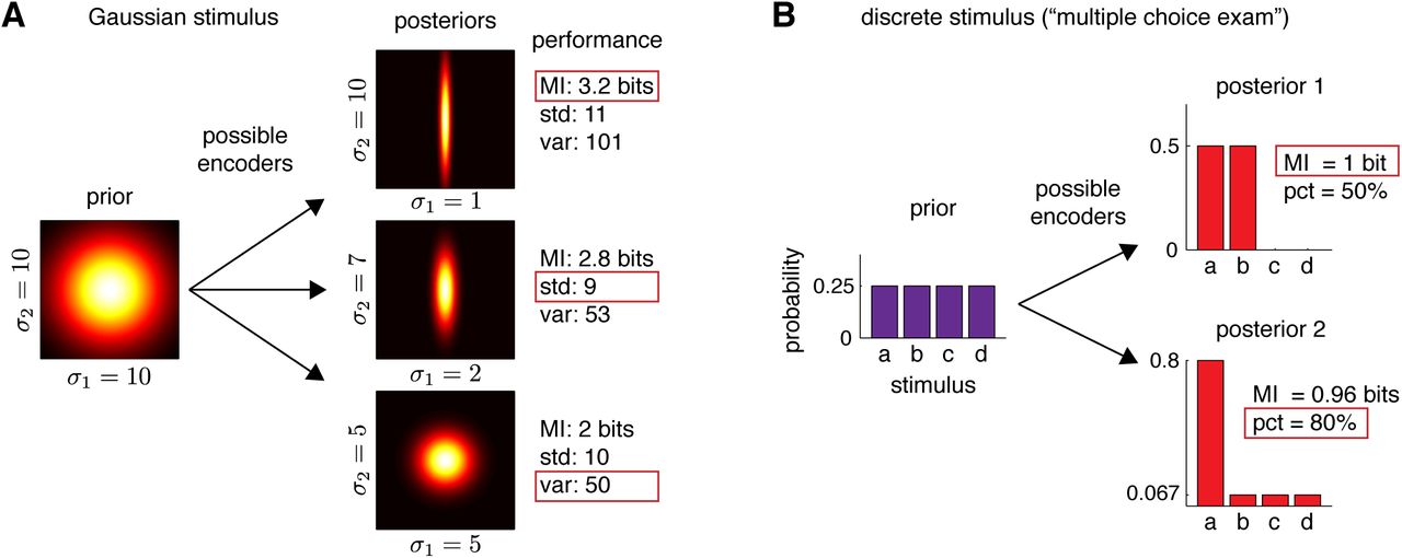
To illustrate the role played by the loss function in Bayesian efficient codes, we first consider a simple example with two neurons encoding a bivariate Gaussian stimulus (Fig. 2A). Suppose that a 2D stimulus x = (x₁, x₂) has an independent Gaussian distribution with standard deviation 10 in both directions. Then consider three possible noisy encoders, each of which corresponds to making a measurement of x corrupted by additive Gaussian noise:

Figure 2: Optimal encoding depends critically on choice of loss function.

(A) Illustration showing three possible encoders of a stimulus with an independent bivariate Gaussian prior distribution. The encoders produce three different Gaussian posteriors, shown at right. For axis-aligned Gaussian distributions, the entropy depends on the product of standard deviations σ₁σ₂, whereas the “total deviation” depends on the sum of standard deviations σ₁ + σ₂, and total variance depends on the sum of variances . According to entropy loss, the top encoder is best (achieving a mutual information of log₂(10 · 10) − log₂(10 · 1) = 3.2 bits), but for total-deviation loss, the middle encoder is best (achieving ), and for total-variance loss, the bottom encoder is best (achieving σ² + σ² = 50). (B) Discrete encoding example, showing two possible encoders for a multiple-choice exam. The prior is an equal p = 1/4 probability for each of the four possible stimuli {a, b, c, d}. The top encoder eliminates two possibilities so that the posterior assigns probability p_i = 0.5 to two stimuli and 0 to the other two. The bottom encoder gives a posterior distribution with probability p_i = 0.8 for one stimulus and the remaining 0.2 probability spread evenly among the other three. The top encoder is optimal for information theoretic loss, since it achieves a mutual information of 1 bit, vs. only 0.96 bits for the bottom encoder. However, for “percent correct” loss, which is sensitive only to max({p_i}), the bottom encoder is clearly better. It identifies the correct stimulus 80% of the time (good for a grade of B-), whereas the top encoder achieves only 50% (an F).

• encoder 1: y₁ = x₁ + ϵ, ϵ ∼ 𝒩 (0, 100/99).

• encoder 2: y₁ = x₁ + ϵ₁, y₂ = x₂ + ϵ₂, ϵ₁ ∼ 𝒩 (0, 100/49), ϵ₂ ∼ 𝒩 (0, 700/93).

• encoder 3: y₁ = x₁ + ϵ₁, y₂ = x₂ + ϵ₂, ϵ₁ ∼ 𝒩 (0, 100/19), ϵ₂ ∼ 𝒩 (0, 100/19).

The first encoder makes a low-noise measurement of x₁ and ignores x₂, whereas the other two encoders distribute noise more or less evenly across x₁ and x₂, resulting in posteriors with standard deviations (σ₁ = 1, σ₂ = 10), (σ₁ = 2, σ₂ = 7), and (σ₁ = 5, σ₂ = 5), respectively, as depicted in Fig. 2A.

It should be obvious from this example that there is no clear sense in which any of these posteriors can be declared better in general. The three posteriors differ in how uncertainty is distributed across the two stimulus dimensions; which is better depends entirely on what the organism cares about. To make this concrete, we consider three loss functions: the posterior entropy, L₁ = − log(2πe σ₁σ₂), (equivalent to maximizing mutual information), the total standard deviation, L₂ = σ₁ + σ₂, and the total variance, . Each loss function gives a different best encoder. The first encoder achieves the smallest entropy, and therefore achieves the highest mutual information between stimulus and response, even though it entirely ignores x₂. The second encoder achieves minimal total-deviation loss, because 2+7=9 (encoder 2) is less than 1+10=11 (encoder 1) or 5+5=10 (encoder 3). The third encoder minimizes total-variance loss L₃, because 25 + 25 = 50 is smaller than either 1 + 100 = 101 (encoder 1) or 4 + 49 = 53 (encoder 2).

This simple example illustrates the manner in which different loss functions give rise to different notions of optimal coding. The loss functions differ in how they penalize the allocation of uncertainty across stimulus dimensions. Entropy is only sensitive to the product σ₁σ₂, which corresponds to the volume of the posterior. We could stretch the posterior by an arbitrary constant a in one dimension and by 1/a in the other, and we would not affect entropy. The other two loss functions, on the other hand, seek to minimize the summed uncertainty (standard deviation or variance) along the two axes. Compared to the entropy, they disfavor posteriors with large uncertainty in one direction, an effect that is larger for variance than for standard deviation. For Gaussian posteriors, they can also be interpreted as minimizing error in an optimal decoder. Minimizing total standard deviation is equivalent to finding an encoder that minimizes the summed absolute error of a decoded estimate: , where is an estimate that minimizes the ℓ₁ error . Similarly, minimizing total variance is equivalent to minimizing the mean squared error of an optimal decoder: , where is the posterior mean¹, also known as the Bayes’ least squares (BLS) or minimum mean squared error estimator.

We could of course have considered other loss functions that would have given us different reasons for preferring any of these three encoders. For example, a “minimax” loss function L = max(σ₁, σ₂), which cares only about minimizing the worst possible performance in any dimension, would also favor the third encoder. Thus, optimality is in the eye of the loss function, and for any set of encoders there may be multiple ways to regard them as optimal in a Bayesian sense.

3.2 Discrete example: multiple choice exam

As second example, consider the case of a discrete stimulus that takes on one of four possible values {a, b, c, d}, each with prior probability 0.25, and a noisy neuron that can respond with 1, 2, 3, or 4 spikes. We will consider the following two possible encoding rules (See Table 1 and Fig. 2B).

Table 1:

Discrete encoding for multiple choice test

The first encoder maps stimuli a and b to responses 1 and 2 randomly with equal probability, and similarly maps stimuli c and d to responses 3 and 4. The second encoder, on the other hand, maps a → 1, b → 2, c → 3, d → 4 with probability 0.8, and with probability 0.2 maps to one of the other three responses selected at random. Fig. 2B shows the kinds of posteriors that arise under these two encoders—these are in fact equal to the rows of the encoding tables given above, since the prior is uniform and each row already sums to 1. For the first encoder, the posterior assigns probability 0.5 to two stimuli and rules out the other two. For the second encoder, the posterior concentrates on one stimulus with probability 0.8, and spreads the remaining 0.2 evenly across the other three stimuli.

It is now interesting to consider which of these two encoders is best according to different loss functions. First, let us consider posterior entropy, which corresponds to maximizing information as in Barlow’s classic definition. The prior has an entropy H(x) = −4 × 0.25 log₂ 0.25 = 2 bits. The mean posterior entropy of the first encoder H(x|y, θ₁) = −2 0.5 log₂ 0.5 = 1 bit, so the mutual information between stimulus and response is 1 bit. By contrast, the posterior entropy of the second encoder is H(x|y, θ₂) = −0.8 log₂ 0.8 − 0.2 log₂(0.2/3) = 1.04 bits, which gives mutual information of only 2 − 1.04 = 0.96 bits. This means that the second encoder preserves strictly less Shannon information about the stimulus than the first, so the first encoder is more efficient². A second natural choice of loss function, however, is the “percent correct”, defined as the percent of the time a maximum a posteriori decoder chooses the correct stimulus. According to this loss function, the second encoder is clearly superior, since 80% of the time it concentrates on the correct stimulus, whereas the best possible decoding of responses from the first encoder can only answer correctly 50% of the time.

This example has perhaps greater cultural and psychological salience if we reframe it terms of students studying for a multiple choice exam. Each question on the exam will have four possible choices (a, b, c, and d), which occur equally often. Student 1 adopts a study strategy that allows her to rule out two of the four choices with absolute certainty, but to have total uncertainty about which of the two remaining options is correct for each exam question. Student 2, on the other hand, adopts a study strategy that allows her to know the correct answer 80% of the time, but has uniform uncertainty about the remaining three options, which are correct the remaining 20% of the time. Which student’s strategy is better? If we judge them according to mutual information, the first student has clearly learned more; her brain has stored 0.04 more bits about the subject matter than the second student. However, if we judge them according to the number of questions they can answer correctly on the exam, the second student’s strategy is clearly better: her expected grade is a B-, with a score of 80%, whereas the second student is expected to fail with only half the questions answered correctly.

An interesting corollary of this example, therefore, is that although information-theoretic learning (cf. [12, 46]) is optimal for True/False exams, it can be substantially sub-optimal for multiple-choice exams.

4 Linear receptive fields

Now we turn to an application motivated by biology. Neurons in the early visual system are often described as performing an approximately linear transformation of the light pattern falling on the retina. A large body of previous work has examined the optimality of these linear weighting functions under the efficient coding paradigm and its variants [10, 15, 16, 18, 33, 47–52].

Here we re-examine this problem through the lens of Bayesian efficient coding. We consider the following simplified model for linear encoding of sensory stimuli: In this setup, we assume that the stimulus, an image consisting of n pixels, is encoded into a population of n neurons via a weight matrix W. Each row of W corresponds to the linear receptive field of a single neuron. For tractability, we assume that the stimulus has a Gaussian distribution (with covariance Q defining the correlations between pixels), and the neural population response is corrupted by additive Gaussian noise with covariance R. We impose a power constraint on the response, corresponding to a bound on the sum of squared responses y. This is a common choice of constraint in the efficient coding and engineering literature due to differentiability and analytic tractability [29, 47]. In practice, the power constraint restricts the model from achieving infinite signal-to-noise ratio by growing W without bound.

For this model, the marginal response distribution P (y) is Gaussian, y ∼ 𝒩 (0, WQW ^T + R), so the power constraint can be written in terms of the trace of the marginal covariance: The posterior distribution P (x|y) is also Gaussian, 𝒩 (µ, Σ), with mean and covariance In this setup, the coding question of interest is: given stimulus covariance Q, noise covariance R, and power constraint c, what is the optimal linear encoding matrix W ? That is, what receptive fields are optimal for encoding of the stimuli from P (x) in the face of noise and a constraint on response variance? Here we consider two possible forms for the loss functional: where are the eigenvalues of posterior covariance Σ, or the variances of the posterior along its principal axes.

The first loss function, posterior entropy, corresponds to classic infomax efficient coding, since minimizing posterior entropy corresponds to maximizing mutual information between stimulus and response. The second loss function, which we term covtropy due to its similarity to entropy, is the summed p’th powers of posterior standard deviation along each principal axis. Like entropy, the covtropy depends only on the eigenvalues of the posterior covariance matrix, and is thus invariant to rotations (See Supplementary Information). For p = 2, covtropy corresponds to the sum of posterior variances along each axis; minimizing it is equivalent to minimizing the mean squared error [15–17] (see Appendix 6.4 for proof).

For p = 1, covtropy corresponds to a sum of standard deviations; this penalizes a posterior with large variance in one direction less severely than covtropy with p = 2. In the limit p → 0, minimizing covtropy is identical to maximizing mutual information, since . In this limit, the optimal code minimizes the sum of log standard deviations, ∑_i log σ_i, which is equivalent to minimizing the product Π_i σ_i. The other interesting regime to consider is the limit p → ∞. In this regime, minimizing covtropy is equivalent to minimizing max_i{σ_i}, the maximal posterior standard deviation, a form of “mini-max” encoding. The optimal code is therefore the one that achieves smallest maximal posterior standard deviation in any direction.

Note that for the linear Gaussian model considered here, the posterior covariance Σ is independent of the response y. This makes the problem easier to analyze because there is no need to compute average loss over the response distribution P (y) (eq. 1). We show here that there is an analytic solution for the optimal linear encoding matrix W in this setting, for both infomax loss and covtropy loss (with any choice of p > 0), if we assume that Q, R, and W have a common diagonalization. This condition arises naturally for a convolutional code, that is, W contains a single receptive field shape that is circularly shifted by one pixel for each neuron in the population, and noise is spatially shift invariant (i.e., R is a circulant matrix). In the following, we examine the properties of Bayesian efficient linear receptive field codes for both information-theoretic and covtropy loss functions (derivation in the Supplementary Information).

4.1 Infomax encoding

The optimal weight matrix W for infomax coding is given by: where c is the power constraint and d is the number of stimulus dimensions. For this encoder, the responses y are perfectly whitened, meaning the response covariance is proportional to the identity, 𝔼[yy^T] ∝ I, and the posterior covariance of x|y is proportional to the product of signal and noise covariances, Σ ∝ (QR).

4.2 Minimum covtropy encoding

For covtropy loss with exponent p, the optimal encoding weights W are given by where constant simply enforces the power constraint. For these weights, the marginal covariance is which implies that optimal responses can be more or less correlated than the stimulus. For example, when noise covariance R is proportional to stimulus covariance Q, then for p = 2 (minimum mean-square error encoding), the optimal receptive fields perfectly preserve the correlations in the stimulus, that is cov[Y] ∝ Q. For p > 2, the optimal receptive fields increase correlations so that responses are more correlated than the stimuli (See Fig. 3). Although the responses become more correlated with increasing p, the posterior covariance, given by becomes increasingly white (i.e., uncorrelated) with increasing p, due to the fact that lim_a→0 M^a = I for any nonsingular matrix M. This results in a posterior with the same uncertainty in all directions, regardless of the prior or noise covariance, in accordance with the “minimax” property for p = ∞ noted above.

Figure 3: Bayesian efficient codes for a linear receptive field model with Gaussian noise.

(A) Gaussian stimulus distribution with strong correlations (ρ = 0.9), with 50 samples shown (blue dots). (B) Neural responses (red dots) corresponding to optimal representations under infomax and covtropy loss functions, under infinitesimal Gaussian noise with covariance proportional to the stimulus distribution. Responses are uncorrelated (“white”) for the infomax encoder, but unchanged for the p = 2 (minimum variance) encoder and stronger for p = 4. (C) Posterior distribution shape for each optimal encoder, showing that the infomax encoder achieves small posterior entropy using a long narrow posterior, whereas optimal covtropy posteriors grow more spherical with increasing p. (D) Relative performance of each encoder according to the loss function considered, normalized so the optimum is 1. Each encoder does best according to its own loss function, and the fall-off in efficiency between infomax and covtropy encoders is substantial; the infomax coder captures almost twice as much information as the p = 4 covtropy encoder in terms of bits (left plot), while the infomax coder exhibits nearly 4 times higher p = 4 covtropy than the optimal p = 4 encoder (right plot).

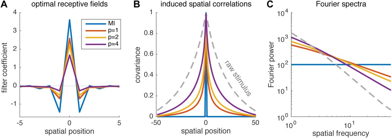
Fig. 4 shows shape of the optimal high-dimensional linear RF for encoding stimuli with naturalistic (1/f ²) power spectrum in a population of neurons with independent noise. Even in the high-SNR regime (when noise is infinitesimal), where perfect whitening maximizes mutual information, the optimal RFs under covtropy loss give less whitening as a function of increasing covtropy exponent p.

Figure 4: Optimal linear receptive fields for different loss functions.

(A) Optimal 1D linear receptive fields for a neuron population with (infinitesimal) independent Gaussian noise and correlated Gaussian stimuli with power spectrum proportional to 1/f ². Plots show central 10 elements of optimal 100-element RFs optimized for mutual information (MI) and covtropy with p = 1, 2, 4. (B) Auto-correlation of the stimulus (dashed) and the 100-neuron population response generated by each encoder. The infomax filter induces perfect whitening so that the autocorrelation is a delta function (blue), while optimal covtropy encoders induce only partial whitening (even in the regime of high SNR). (C) Fourier power spectrum of stimulus and population responses, showing that optimal covtropy populations induce partial whitening, preserving more low frequency information.

5 Nonlinear response functions

So far we have focused on encoders that linearly transform the stimulus. However, many neurons exhibit rectifying or saturating nonlinearities that map the raw stimulus intensities so as to make optimal use of a neuron’s limited response range.

5.1 Noiseless quantized response

Barlow’s efficient coding theory states that the nonlinearity should map the stimulus distribution so as to maximize information between stimulus and response [2, 31], which naturally depends on the prior distribution over stimuli, the conditional response distribution, and the particular constraint on neural responses. For the case of noiseless responses and a simple constraint over the range of allowed responses, the shape of the information-maximizing nonlinearity is proportional to the cumulative distribution function (CDF) of the stimulus distribution, producing a uniform marginal distribution over responses [53].

In a groundbreaking paper that is widely considered the first experimental validation of Barlow’s theory, Simon Laughlin [27] measured graded responses from blowfly large monopolar cells (LMC) to contrast levels measured empirically in natural scenes. Laughlin found that the LMC response nonlinearity, measured with responses to sudden contrast increments and decrements, exhibited a striking resemblance to the shape of the empirically measured CDF of contrast levels in natural scenes. Fig. 5A shows a reproduction of the original figure, showing that the non-linear response is closely matched with the stimulus distribution expected by the infomax solution.

Figure 5: Bayesian efficient coding for noiseless nonlinear transformations applied to LMC response.

(A): Measured large monopolar cell (LMC) response from [27] and the cumulative distribution function of the stimulus statistic. The two lines should be identical for optimal encoding under the infomax criterion. (B) Sigmoid fits for curves in panel A, and four predicted nonlinear encoders based on the sigmoid fit of the stimulus distribution. (C) Predicted response marginals under four different optimal codes using P (x) in panel B, and the marginal distribution estimated from empirically measured g.

Here we re-examine Laughlin’s conclusions by analyzing the same dataset through the enlarged framework of Bayesian efficient coding. We can formalize the coding problem as: Here x is a scalar stimulus with prior distribution P (x), and the encoding model is described by g(x), a noiseless, quantizing transformation from stimulus to discrete response levels. Note that some information about the stimulus is lost due to quantization error. For classical infomax encoding, we know that optimal g performs histogram equalization by taking on the quantiles of P (x), resulting in a uniform marginal response distribution P (y) [27, 53].

We extracted the stimulus distribution from ([27], Fig. 2) in order to determine the optimal nonlinearity under Bayesian efficient coding paradigms for several different choices of loss function. In particular, we considered the L_p-”norm” reconstruction error function of the form: where p ≥ 0 and is the Bayesian optimal decoder for x from y [54]. For p = 2, this loss is equivalent to the mean squared error, and estimate is equal to the mean of the posterior over x given y. Smaller values of p correspond to reducing the relative penalty on large errors and increasing the relative penalty on small errors; in the limit of p → 0, the loss converges to posterior entropy, making it equivalent to the infomax setting [24, 54].

We used numerical optimization to find the optimal nonlinearity g(x) for (see Methods). We plotted these Bayes optimal nonlinearities against the infomax nonlinearity from Laughlin, as well as the empirically measured LMC response nonlinearity (Fig. 5B). Although the infomax nonlinearity resembles the true nonlinearity by eye, close inspection reveals the BEC nonlinearity with provides a much closer fit. This means that the LMC response function is more accurately described as minimizing average decoding error raised to the one-half power than as maximizing information.

The difference between infomax and loss appears slight when viewed in terms of the optimal nonlinearity g(x), but is more dramatic when we consider the predicted marginal distribution over responses P (y) (Fig. 5C). We fit the neuron’s true response nonlinearity with a sigmoid function (Naka-Rushton CDF; See Methods), and computed the predicted marginal response distribution P (y) for each nonlinearity g(x). As expected, the infomax nonlinearity (dashed trace) produces a flat (uniform) distribution over response levels. However, both the non-linearity and the predicted LMC response distribution exhibit a noticeable peak around intermediate response levels, with intermediate response levels used more often, and responses at the extreme left and right tails used less often. We note that such peaking is expected under loss functions that penalize the magnitude of decoding errors. In fact, the optimal nonlinearities for p = 1 and p = 2 generate responses distributions that are even more peaked than the real data, since they assign less probability mass to outermost response levels, where decoding errors are largest. The infomax loss function, by contrast, ignores the size of errors and simply seeks to match quantiles of the stimulus distribution.

5.2 Linear-Nonlinear-Poisson spiking

In the previous example, we assumed no variability in the neural response, but what if there are? We employ a sensory encoding scheme with random spiking noise in addition to nonlinear transformation to demonstrate the general principles of BEC. We consider the following linear-nonlinear-Poisson (LNP) model [55]. where g(·) ≥ 0 is a scalar non-decreasing function, and with a marginal firing rate constraint C = 𝔼[y] = ĉ where ĉ is the empirical mean rate. Unlike the linear receptive field with gaussian noise case discussed earlier, this form is no longer analytically tractable. Hence, we once again use numerical optimization to find the optimal nonlinearity g from spikes.

To compare with the theory, we analyze the responses of a blowfly H1 neuron that encodes horizontal visual motion [56]. The visual motion stimulus were white Gaussian noise. We first projected the spike trains onto the spike-triggered average and binned with 25 ms window to produce spike counts (Fig. 6A). The mean firing rate constrained infomax nonlinearity for this model shows threshold like behavior and far from the empirical nonlinearity (Fig. 6A) obtained via Gaussian process regression [57]. With the constraint on g to be non-decreasing and the marginal mean firing rate to match the data, we inferred the optimal g under the class of L_p-norm loss function given by eq. 17. For small values of p, the optimal nonlinearity behaves like a smooth step function, and for large p, it behaves as a rectified linear function (Fig. 6B). We found that the optimal nonlinearity is most similar to the empirical one for p = 4 (Fig. 6B). Note that the corresponding response distributions are no longer uniform nor Poisson (Fig. 6C). This dataset was also analyzed by Wang and coworkers [58] with similar but distinct assumptions and methods.

Figure 6: Bayesian efficient coding for linear-nonlinear-Poisson model applied to H1 response.

(A) Blowfly H1 neuron response to white noise from [56]. Black curve shows a Poisson-Gaussian process fit of the noninear rate function, while dashed curve shows the numerically obtained infomax solution. The stimulus has been filtered with spike-triggered-average (STA) and binned at 25 ms bin. 1% of the samples are plotted as blue jittered dots. (B) Optimum nonlinear encoders for L_p-norm reconstruction loss with mean firing rate constraint. (C) Predicted response marginals under optimal codes corresponding to panel B and the marginal distribution from spike data.

6 Discussion

We have synthesized Barlow’s efficient coding hypothesis with the Bayesian brain hypothesis in order to formulate a Bayesian theory of efficient neural coding. In this theory, an efficient neural code corresponds to an encoding model that produces optimal posteriors over stimuli under a capacity constraint on the neural response. The optimality of the posterior is determined by a loss function L, and the choice of loss function can have major effects on the optimal code. We have shown that Barlow’s original theory corresponds to a special case of this theory in which the loss function is the Shannon entropy of the posterior, corresponding to codes that maximize mutual information between stimulus and response. However, such codes may be inefficient with respect to loss functions that are sensitive to the shape of the posterior, or the size of different decoding errors.

To illustrate our framework, we have derived Bayesian efficient codes for two canonical neural coding problems: (1) population encoding of high-dimensional stimuli with linear receptive fields; and (2) single-neuron encoding of low-dimensional stimuli with a nonlinear response function. In the first case, we showed that the “whitening” solution favored by classic efficient coding can be sub-optimal for other loss functions, and that even in the high-SNR (signal-to-noise ratio) regime, optimal codes may increase the correlations between neurons. In the second case, we re-examined the classical results of Laughlin, and showed that the nonlinear response functions of the blowfly LMC neurons are in fact more consistent with a Bayesian efficient code that minimizes the average square root of the decoding error than a code that maximizes mutual information. While these two examples are both highly simplified, they illustrate the power of this general formulation of efficient coding, and show surprising and non-intuitive results that contrast with previous findings.

6.1 Relationship to previous work

In the years since the seminal papers of Attneave and Barlow, a large literature has taken up the problem of optimal neural coding, spanning a wide range of both information and non-information-theoretic frameworks. Barlow’s original paper considered noiseless encoding, where each stimulus maps to a deterministic response [2]. Atick and Redlich extended this framework to incorporate noise, deriving the remarkable result that optimal receptive field shapes change with SNR, consistent with observed changes in retinal ganglion receptive fields [10]. They showed that whitening is optimal only at high SNR, and that optimal responses become correlated at lower SNR—note that this differs from our result showing that whitening can be sub-optimal even at high SNR for other loss functions (Figs. 3 & 4).

Several alternate versions of efficient coding based on information theory were advanced in the early years. Barlow first proposed that neurons optimize a quantity he called redundancy, given by 1 − I(x, y)/C, or one minus the mutual information divided by the channel capacity C [2]. (In fact, Barlow referred to his theory as the “redundancy reduction hypothesis”, and the more common “efficient coding hypothesis” label has only appeared more recently, e.g., [59]) Atick and Redlich modified Bar-low’s theory to replace the C in the denominator by C_out, a modified notion of channel capacity related to the system’s total power, which they held to be more biologically plausible [10, 48]. Neither theory therefore amounted to a pure “infomax” hypothesis, such as that advanced by [8], since optimality could be increased either by increasing mutual information or decreasing the channel capacity C or C_out in the denominator.

It bears mentioning that Barlow’s definition of redundancy has no relationship to the concepts of redundancy and synergy later introduced by Brenner and colleagues, which quantify whether groups of neurons encode more or less information jointly than separately [60–63]. An efficient code according to Barlow or Atick & Redlich may be perfectly efficient in the sense of maximizing the ratio of information to capacity, while being either redundant or synergistic in the (more widely used) sense defined by Brenner et al [64].

Theories of efficient coding based on information-theory have been applied to a wide variety of different sensory systems and brain areas. These can be roughly grouped into those focused on linear receptive fields [32, 35, 65, 66], those focused on tuning curves [23–26, 51, 67–70], and those addressing some aspect of population coding, such coupling strengths between neurons [71, 72]. A substantial portion of this literature work has approached the problem of optimal coding through the lens of Fisher information [23, 24, 26, 58, 67, 69], although Fisher information may not accurately quantify coding performance in low SNR settings (e.g., short time windows or low firing rates) [17, 22, 25, 73].

A substantial literature has also considered optimal coding under alternate loss functions, and recent work has shown that codes optimized for mutual information may perform poorly for non-information-theoretic loss functions [74]. The most well-studied alternate loss function is the squared loss, , which results in so-called “minimum mean squared error” codes; such codes achieve minimum expected posterior variance (as opposed to minimum posterior entropy). These codes have received substantial attention in both engineering [75, 76] and neuroscience [15, 16, 18, 22, 25, 77]. Optimal codes for a wide variety of other losses or optimality criteria have also been proposed, including: minimization of motor errors [14], maximization of accuracy [78–80], optimal coding for control applications [81], and optimal future prediction [12, 82–86], and loss based on natural selection [6]. Other recent work has considered codes that maximize metabolic efficiency [11, 13], which in our framework corresponds more naturally to the constraint (which is concerned with use of finite resources) than the loss function (which is concerned with the posterior distribution).

In the statistics and decision-making literature, our work is closely related to Bayesian statistical decision theory [87–89], although such work has tended not to consider the problem of optimal sensory coding. One noteworthy difference between our framework and classical Bayesian decision-making theory is that the loss functions in decision theory are typically defined in terms expected cost of a point estimate (e.g., mean-squared error or percent correct). In our framework, by contrast, the loss is defined as a functional of the posterior, that is, an abitrary integral over the posterior distibribution. This allows us to consider a wider class of loss functions, such as the posterior entropy or the average posterior standard deviation, which cannot be written in terms of an expected loss for a point estimate of the stimulus. Thus, our loss function merely specifies what counts as a good or desirable posterior distribution, without assuming how the posterior will be used (e.g., to generate a point estimate).

6.2 Relevance of Shannon information theory

Shannon’s information theory holds a special status in engineering, signal processing, and other fields due to its universal implications for communication, compression, and coding in settings of perfect signal recovery. However, it is unclear whether information-theoretic quantities like entropy and mutual information are necessarily relevant to information processing and transmission in biological systems [90]. In particular, Shannon’s theory (1) requires complex computation and long delays to encode and decode in ways that achieve optimality [5]; (2) ignores biological constraints (e.g., neurons cannot implement arbitrary nonlinear functions); (3) applies to settings of perfect signal recovery, which may not be possible or even desirable in biological settings.

In the Bayesian efficient coding, the encoder is selected from a biologically relevant parametric family. And although we consider the (negative) mutual information as one possible choice of loss function, there is no a priori reason for preferring it to other loss functions; as we have shown, optimizing MI it will not necessarily give good performance for other losses (e.g., Figs. 2 & 3). We therefore find no justification for claims (commonly found in the neuroscience literature) that, in the absence of knowledge about the brain’s true loss function, it is somehow best to maximize mutual information.

A framework more relevant to sensory coding in the nervous system is Shannon’s rate distortion theory for lossy encoding [28]. Given an allowed maximum distortion (as a measure of encoding-decoding error) L^∗, the rate distortion function R(L^∗) describes the minimum necessary mutual information of the channel (implemented by the encoder-decoder pair) to achieve it: . One can prove that the more mutual information is allowed, the smaller the achievable distortion; in fact R(L^∗) is a non-increasing convex function [29]. This provides an interesting overlap between the two theories: a sub-class of BEC with mutual information constraint can be reformulated as a special case of rate distortion theory. Consider the following dual formulations: where is the loss given in eq. 1. The rate distortion solution θ_RD coincides with the BEC solution θ_BEC, because the distortion function is monotonically decreasing. Although this provides a insightful connection, such relations do not always exist, and more generally it is not clear why a bound on mutual information would be a biologically relevant constraint on a sensory encoder.

6.3 Application to experimental data

In this manuscript, we used the BEC framework to identify loss functions consistent with neurophysiology datasets. To accomplish this, we searched for the optimal encoding model under different choices of loss function, and asked which of the resulting encoding models most closely resembled the empirical encoding model. Although both of our examples came from the early visual system, one could apply the same approach to datasets from any sensory modality (e.g., audition, olfaction, somatosensation). This would reveal what loss function (if any) the neurons in different brain and different modalities seek to optimize. Researchers can therefore test whether neural representations maximize mutual information (as posited by classic efficient coding) or some other loss metric.

A second way to apply the BEC framework to data is to identify the prior distribution for which an observed sensory encoding is optimal (cf. [42, 54, 91]). In this case, we would take the encoding model parameters inferred from neurophysiological data and optimize the prior distribution under differerent fixed choices of loss functions or constraints. The inferred priors may then serve as predictions of the distribution of natural signals for which the system is optimized, or as an assay of neural adaptation in experiments with time-varying stimulus statistics.

Finally, the BEC framework could be used to test which constraints are most relevant to a particular neural code. Here we assumed that the relevant constraint was on the range (for analog responses; Fig. 5), or on the mean firing rate (spiking responses; Fig. 6). However, one could test whether observed responses are more consistent with alternate sets of constraints, including metabolic or energetic constraints [13, 54], constraints on higher-order response statistics [92], or architectural constraints on the model parameters (e.g. sparsity, wiring length) [71, 93, 94].

The general domain of application of BEC is thus the same as classic efficient coding; the key difference is that BEC has one additional “knob” that can be tuned, namely the loss function. As classical efficient coding provided new explanations for adaptation and sparse coding, the BEC framework can be used to extend and refine such hypotheses, set free from the restrictive assumption that mutual information is the relevant loss function for all of behavior.

6.4 Limitations and future directions

What cost or loss function is the nervous system optimizing for? We emphasize that BEC alone cannot serve as a normative theory to answer this question; each problem and environment should dictate the loss functional and prior. Rather, BEC should be used as a guiding principle that frees the theory of efficient coding from its traditional reliance on information theoretic principles, and to cover an appropriately broad range of theories of optimal neural encoding.

BEC on its own has many degrees of freedom and is likely under-constrained by current neural and behavioral observations. Moreover, different combinations of constraints and loss functions may be consistent with a single encoding model, providing multiple “optimal” explanations for a single encoder. The priors, encoding models, constraints, and loss functions we have considered here were guided primarily by tractability as opposed to neural or biological plausibility, but some of these components (e.g., prior and noise) can be quantified with measurements [36, 95, 96]. We can start to make reasonable inferences about constraints and loss functions through careful study of the brain’s resource consumption [97, 98] or the behavioral consequences of different kinds of errors [99–101].

A variety of other issues relating to normatively optimal neural coding remain to be addressed by our theory:

Computational demands

the BEC framework does not consider constraints on the brain’s computational capabilities. In particular, our theory—like with the Bayesian brain hypothesis itself—assumes that the brain can compute the desired posterior distribution over stimuli given the response, or at least extract the posterior statistics needed for optimal behavior. This is almost certainly not the case for many of the complex inference problems the brain faces. It seems more likely that the brain relies on shortcuts, heuristics, and approximate inference methods that result in sub-optimal use of the stimulus information contained in neural responses relative to a Bayesian ideal observer [102]. The BEC paradigm could therefore be extended to incorporate computational constraints: for example, linear readout of neural activity is linear, or the use of particular approximate Bayesian inference methods [103]).

The role of time

we have focused our analyses on coding problems that follow the sequential nature of Bayesian inference (stimulus → response → posterior distribution) and have ignored the continuous-time nature of stimuli, responses, and behavior. However, there is nothing about our theory that precludes application to continuous-time problems, and previous work has formulated population codes capable of updating a posterior distribution in continuous time [104–108]. In many cases optimal coding depends on the timescale over which information is integrated: for example, previous work has shown that optimal tuning curve width depends on the time over which spikes are generated, with longer time windows necessitating narrower tuning [17, 25]. Recent work has discovered limits on fast timescale transmission of information in physical and biological systems [109], but there is still a need for a theory of optimal coding in settings where there is uncertainty about the time (or times) at which the posterior distribution will be evaluated or “read out”.

Latent variables

we have not so far discussed latent variable models, in which there are additional unobserved stochastic components affecting either the stimulus or the neural response. In stimulus latent variables models, the quantity of interest is a latent variable z that may be regarded as underlying or generating the sensory stimulus x. (For example, z might the velocity of an object or the identity of a face, and x is the resulting image or image sequence presented to the retina [110]). In such settings, the posterior over the latent variable z might be the quantity of interest for an optimal code; BEC can handle this case by defining a loss function sensitive to the posterior p(z|y). This can be seen as a valid instance of BEC because this distribution can be written as a functional of the stimulus posterior: p(z|y) = ∫ p(z|x)p(x|y) dx, where p(z|x) is the posterior over the latent given the stimulus under the generative model. Latent variables also arise in models of neural activity with shared underlying variability [111–114]. In such cases, it is natural to write the encoding model itself as a joint distribution over activity and latents, p(y, z|x); the BEC paradigm can once again handle this case by marginalizing over the latent to obtain p(x|y). Thus, BEC can accommodate both kinds of latent variable models typically used in neuroscience, and the consideration of stimulusrelated latent variables may motivate the design of loss functions are sensitive to particular latent variables while discarding other aspects of the stimulus (e.g., as in the information bottleneck [84] or accuracy maximization analysis [78, 110]).

Although we have focused on two canonical problems that arise repeatedly in the neural coding literature, namely optimal linear receptive fields and optimal nonlinear input-output functions, we hope that future work will address other coding problems relevant to information processing in the nervous system (e.g., multi-layer cascades, dynamics, correlations), and will be extended to non-Bayesian frameworks (e.g., that take into account computational costs or constraints). We believe that the BEC paradigm provides provides a rigorous theoretical framework for neuroscientists to evaluate neural systems, synthesizing the Bayesian brain and efficient coding hypothesis into a formalism that can incorporate diverse optimality criteria beyond classic information-theoretic costs.

Methods

Blowfly LMC data from [27]

We extracted the data points from the figures in the original paper [27] to fit the models in section 5 and for the plots in Fig. 5. The data are available as supplementary data files.

To fit the stimulus CDF and the response nonlinearity of the blowfly LMC, we fit a 3-parameter Naka-Rushton function |(x − a)^b|/(|x − a|^b + c) (plotted as grey dotted line in Fig. 5B) to estimate the stimulus CDF (Fig. 5A). The parameters for the stimulus CDF were a = −1.52, b = 5.80, c = 7.55, and a = −1.90, b = 5.84, c = 37.17 for the LMC response.

To compute the optimal nonlinearities plotted in Fig. 5B, we parametrized the nonlinearity as a piecewise constant function defined on 25 bins, and numerically minimized the loss (eq. 17) using MATLAB’s fminunc to optimize the location of the bin edges for each value of p. To compute the marginal response distributions (Fig. 5C), we transformed the quantization bin edges through the prior CDF.

Blowfly H1 data from [56]

We computed the spike-triggered average (STA) for a history of 120 ms at 1 ms bin size and projected the stimulus on the STA before binning both the projection and the spikes on non-overlapping 25 ms time bins. The empirical nonlinearity (shown in Fig. 6A,B) is estimated using Gaussian-process-Poisson regression. The nonlinearity was parameterized by 100 non-negative firing rates spanning 5 standard deviations around the origin of the projected stimuliaround the origin. Similarly with the LMC data, we then optimized the nonliaerity under different loss functionals using numerical gradient descent with the marginal firing rate constraint (Fig. 6B).

Supplementary Information

Acknowledgments

We would like to thank Jacob Yates and Ozan Koyluoglu for helpful discussions. JWP was supported by grants from the McKnight Foundation, Simons Collaboration on the Global Brain (SCGB AWD1004351) and the NSF CAREER Award (IIS-1150186). IMP was supported by the Thomas Hartman Center for Parkinson’s Research (64249), the NIH NIBIB R01 EB-026946, and the NSF CAREER Award (IIS-1845836).

Appendix A: Encoding models for multiple choice exam

Appendix B: Loss functionals

Loss functionals quantifies the goodness of the posterior distribution P (x|y, θ). There are broadly two classes of loss functionals: entropic loss or reconstruction loss. Entropic losses quantify the average uncertainty of the posterior: More concentrated the posterior, the better. Both eq. 1b and eq. 1c converges to eq. 1a in the limit of α → 1.

Traditional entropic losses do not discriminate points in the stimulus domain, that is, any error is treated equally. However, when stimulus space is ℝⁿ, it makes sense to prefer locally tight posterior distributions. One such measure is the p-covtropy which measures the posterior concentration around the posterior mean (only defined for distributions in ℝ^d). Note that ‘th power of the posterior covariance matrix corresponds to taking p’th power of the standard deviations along each principal axis through diagonalization.

The second class of loss functionals depend on a specific readout (a.k.a. estimator or reconstruction) that maps the neural response y back to the stimulus domain. We consider a general average reconstruction error loss functional of the form: where d(·, ·) is a distortion measure. Mean squared error and the 0-1 loss are widely used in communication theory, machine learning, and statistics in general.

There are loose bounds that connect the posterior entropy with Bayesian error rate (e.g. Fano bound for classification) [76]. However, these bounds do not justify infomax strategy because better Bayesian error rate can be achieved with a system that directly optimizes for the target error measure.

Note the similarity between p-norm error and the p-covtropy when posterior mean is used for decoding. They coincide when p = 2, however for p ≠ 2, unlike the p-norm error, p-covtropy is invariant under unitary transformation of the stimulus space (which is the key difference between the 2D Gaussian and the linear receptive field examples). This is an important distinction if axes in x do not have special meaning, and rotated posteriors are considered equally good. We can make this connection rigorous for a Gaussian posterior, x|y ∼ 𝒩 (µ, C). Let C = UDU ⁻¹ be the eigendecomposition of the covariance matrix. Let Z ∼ 𝒩 (0, D) be aligned on the principal axes, the p-th power of the p-norm is given by, where .

In section 4, we discuss the loss functions only for Gaussian posteriors. However, covtropy is well defined for any distribution with a valid covariance matrix. Note that minimizing the limiting case of covtropy for p → 0 and maximizing mutual information do not coincide in general since posterior entropy is not a sole function of the covariance in general.

Appendix C: Equivalence of MSE and covtropy for p = 2

Here we provide a simple proof showing that minimizing covtropy for p = 2 corresponds to minimizing mean-squared error (MSE). Let denote the MSE for any estimator , where expectation is taken with respect to the posterior P (x|y). It is well known that the posterior mean or “Bayes least squares” estimator achieves the minimum of the MSE, which is then given by . We can use identities involving trace and the definition of covariance to show that MSE is equal to , which is the covtropy with p = 2. Thus, the code that achieves minimum p = 2 covtropy corresponds to the code that achieves minimum MSE point estimation of the stimulus.

Appendix D: Linear receptive fields

Here we derive the optimal receptive fields for linear encoding under Gaussian noise (Sec. 4). Recall the model (eqs. 3-5): and we wish to find the optimal W subject to the power constraint We make the assumption that Q,R, and W matrices commute, which means they share a common eigenbasis or can be diagonalized by the same orthogonal matrix. This occurs, for example, if all three are circulant matrices, so that W consists of shifted copies of a single RF shape.

D.1 Infomax

Maximizing information is equivalent to minimizing the posterior entropy: We can find the optimal W subject to the power constraint above using the method of Lagrange multipliers: where λ is a Lagrange multiplier. This implies giving and finally Plugging his solution into the constraint (eq. 5) gives which implies 1/(2λ) = c/n, where n = dim(y) is the number of neurons. Substituting for λ gives the desired expression:

D.2 Minimum p-Covtropy

We can take a similar approach for the loss function we have called p-covtropy, which is effectively the mean p’th power error in the eigenbasis of the posterior distribution. This is given by which involves the posterior covariance matrix Σ to the matrix-power p/2. It turns out this loss function has the same optimum as infomax loss in the limit p → 0.

Once again, the method of Lagrange multipliers allows us to solve for W explicitly in the case that W, R, and Q commute. Taking the derivative of the Lagrangian with respect to W and setting to zero yields This can be simplified to and so and finally with . Substituting Ŵ_p into the power constraint (eq. 5) gives: which achieves the constraint with equality when which completes the derivation.

Footnotes

• revised text, new Fig 6, updated analysis, additional methods detail.

• ¹ Note that this connection between sum of moments and minimization of error does not hold in general. See supplemental information for detail.

• ² Strictly speaking the two channels have different capacity, the definition of redundancy doesn’t apply directly.