

Abstract
A major challenge to studying the neural circuits underlying perceptual decision making has been the limited availability of tools for manipulation of neural activity. In recent years, rodents have emerged as a desirable model for overcoming the technical hurdle. However, mice, which offer abundant genetic tools for circuit manipulation, are underrepresented in perceptual evidence accumulation studies. Here we describe the behavior of mice performing a visual evidence accumulation task similar to one previously used in rats and humans. We found that although mice were capable of achieving similar accuracy levels as rats, differences in accumulation strategy were apparent. To test the engagement of cortex in the visual evidence accumulation task, we optogenetically inhibited activity in the anteromedial (AM) visual area using JAWS. Importantly, light activation biased choices in both injected and uninjected animals. Fortunately, by varying the stimulus-response contingency while holding constant the stimulated hemisphere, we surmounted this obstacle and demonstrated a role for AM in contralateral choices. Taken together, our results argue that mice accumulate visual evidence to guide decisions, an ability that is supported in part by area AM.
Introduction
In recent years, rodents have emerged as a powerful model organism for probing the neural circuit mechanism of perceptual decision making (Carandini and Churchland 2013). In particular, mice have become an ideal model for studying neural circuits because of the abundant tools for accessing and probing genetically defined cell types (Taniguchi et al. 2011; Madisen et al. 2010, 2012, 2015). Despite the advantages available to the mouse model, rats are more commonly used in perceptual decision making studies that involve accumulation of stochastic sensory evidence over time, perhaps due to the assumption that such tasks are too difficult for mice. Mice, however, have been trained on a variety of complex sensory perception tasks (Andermann et al. 2010; Busse et al. 2011; Glickfeld et al. 2013; Guo et al. 2014a; Burgess et al. 2016; Goard et al. 2016; Jeong et al. 2017). Further, recent studies have shown that mice can be trained to achieve similar psychophysical performance levels as rats (Douglas et al. 2006; Jaramillo and Zador 2014). Finally, a growing number of studies have successfully trained mice on temporal evidence accumulation paradigms (Douglas et al. 2006; Sanders and Kepecs 2012; Stirman et al. 2016; Morcos and Harvey 2016; Marbach and Zador 2016) reflecting the growing interest in leveraging the benefits of the mouse model for studying the underlying neural circuits of evidence accumulation. However, it is not established whether mice that perform an evidence accumulation paradigm equally well as rats and are utilizing the same behavioral strategy or neural machinery.
To understand the neural mechanisms that enable evidence accumulation for visual decision making, we tested the causal involvement of secondary visual area AM for behavior. Area AM is a prominent candidate to perform evidence accumulation as it overlaps with previously defined location of mouse parietal cortex (Funamizu et al. 2016; Krumin et al. 2017) and has prominent projections to frontal and motor areas. Similar projection patterns have been observed in primate sensorimotor area LIP (Cavada and Goldman-Rakic 1989a, 1989b), an area routinely implicated in perceptual decision making studies (Gold and Shadlen 2007; Hanks and Summerfield 2017). Thus, AM is in a position to play a key role in translating visual information into motor output. Moreover, the role of AM (and many mouse secondary visual areas) in behavior is unknown. AM could mediate a spatial (motor) bias as it is reciprocally connected with cortical (Wang et al. 2012) and subcortical motor areas (Allen Brain Atlas 2015), which are capable of biasing behavioral response. Alternatively, AM could mediate a sensory bias, for instance, if AM selectively preferred low-or high-rate stimuli. This is an attractive viewpoint given that mouse secondary visual areas have distinct preferences for temporal frequency (Andermann et al. 2011; Marshel et al. 2011; Tohmi et al. 2014).
Results
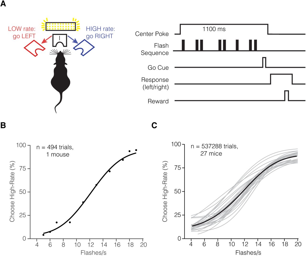
We trained mice to categorize a stochastic pulsatile sequence of visual flashes, similar to earlier studies with rats (Raposo et al. 2012; Brunton et al. 2013; Scott et al. 2015). Briefly, mice performed a three-port choice task (Uchida and Mainen 2003), in which they judged whether the total number of full-field flashes presented during a 1s period exceeded an experimenter-defined category boundary (Figure 1A). Each flash in the sequence was 20 ms long and followed by an inter-flash interval drawn from a discrete exponential distribution (Supplementary Figure 1A).

(A) Task schematic and trial structure of the three-port choice task. The mouse initiated trials and stimulus delivery by poking the center port. The mouse responded to whether the stimulus was low-rate (left port) or high-rate (right port). The mouse had to wait at the center port for at least 1100 ms, with the stimulus delivered after a variable delay (10-100ms). At the end of the 1000ms stimulus period, an auditory “Go” tone was played to inform the subject to make a choice. Correct choices to the left or right were rewarded with a small drop of water (2 μL), incorrect choices were followed by a 2-3 s timeout. (B) Psychometric function fit for individual mouse from single session, and (C) Multiple mice averaged across multiple sessions. Individual mouse (gray traces) and total average (black) n = 27 mice.
Mice learned to categorize stochastic sequences of visual flashes
Mice performed several hundreds of trials per session (Supplementary Figure 1B; median 767 trials) and reached high performance accuracy at the easiest level of the task in less than 20 sessions or 10,000 trials (Supplementary Figure 1C-F). Behavioral training typically lasted approximately 2 months, with one daily session 5 days per week and lasting up to 2 hours per session.
In the first stage of training, mice were trained to self-initiate trials by poking into the center port and remaining in the center port for up to 1100 ms, while the visual stimulus was presented (Figure 1). Training was considered complete when mice waited at least 1100ms at the center port and performed above 80% percent correct on the easiest flash rates (Supplementary Figure 1C, E), and experienced at least 8 or more flash rates. Behavioral performance was quantified by fitting a psychometric function (Figure 1B,C). We evaluated the percentage of trials in which the mouse categorized the given stimulus sequence as “high-rate” (i.e. the number of flashes exceeded the category boundary of 12 flashes/s). Individual mice on single sessions (Figure 1B) and across multiple sessions (Figure 1C) accurately reported more high-rate choices when presented with increasing flash rates, achieving psychometric performance comparable to rats trained on the same task.
Mice decisions were influenced most by flashes early in the sequence
To maximize accuracy, animals should count all the flashes presented during the fixed stimulus presentation period. Because all flashes in the sequence are equally informative about the overall count, subjects should apply an equal weight to all flashes. However, mice might instead pay attention only to the first (or second) half of the stimulus. Attention to flashes early in the sequence would reflect an impulsive strategy of making up one’s mind too early, whereas attention to flashes later in the sequence would reflect a forgetful strategy (Kiani et al. 2008).
We used the well-established logistic regression approach to estimate the psychophysical kernel (Huk and Shadlen 2005; Katz et al. 2016; Yates et al. 2017). The logistic regression-based reverse correlation approach reveals how each incoming flash, on average, influences the subject’s choice. Across mice (Figure 2A), the entire sequence of flashes was informative, as indicated by non-zero regression weights after the first time bin. The first time bin is zero because a flash is always presented at the start of each flash sequence. Interestingly, flashes presented earlier in the sequence generally informed the choice more strongly than flashes presented later in the sequence. This implies that mice tended to over-weight stimuli presented early in the trial, consistent with an impulsive integration strategy. For comparison, the psychophysical kernels of rats (Figure 2B) trained on the same task were generally flat, reflecting an integration strategy in which evidence is integrated equally over time.

(A) Kernels of mice and (B) rats. Gray traces, individual subjects; black trace, average subject.
Mice were influenced by performance on previous trial
Next we evaluated whether mice trained on the evidence accumulation paradigm were influenced by performance on previous trials. Several studies have found that both human and animal subjects performing perceptual tasks are influenced by previous choices (Busse et al. 2011; Fründ et al. 2014; Scott et al. 2015; Abrahamyan et al. 2016; Urai et al. 2017), even when the trials are independent. We used two quantitative models to assess whether mice trained to make categorical decisions about visual pulsatile stimuli were susceptible to choices made on previous trials.
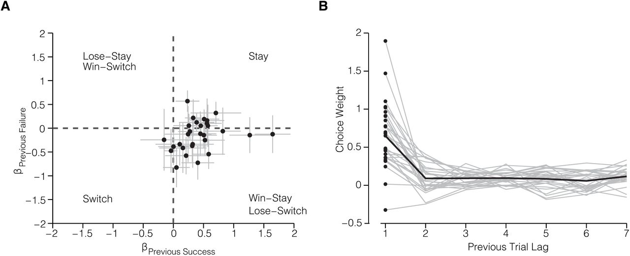
The first approach assessed whether success or failure on the most recent trial influenced the performance on the current trial (Methods; Busse et al. 2011). Figure 3A shows a scatter plot of the coefficients for previous success (βS) and previous failures (βF). All the mice (n = 27) had positive βS coefficients, indicating that mice tended to repeat the same choice on the current trial if they were rewarded on the previous trial. Approximately half the mice had positive βF coefficients, meaning that they mice tended to repeat their choice following a failure (Figure 3A, Stay quadrant), while the other half had negative βF coefficients, indicating a tendency to switch choices following a failure (Figure 3A, Win-Stay, Lose Switch quadrant). The overall observed trial history patterns were similar to those of human subjects performing a perceptual decision making task (Abrahamyan et al. 2016). The second approach evaluated the influence of the history of previous choices on the current choice. The probabilistic model is equivalent to the model described by (Fründ et al. 2014). This model revealed that the most recent choice had the greatest influence on the current choice (Figure 3B).

– (A) Previous choice history: Influence of successes and failures on the current choice for each mouse (n = 27 mice). Coefficients were estimated for each session individually and mean coefficients across sessions are plotted. Error bars represent standard error of the mean. (B) Effect of previous choices (n = 7 trials in the past). Gray traces, individual subjects (n = 27 mice); black trace, average across subjects.
Mice decisions are influenced by cumulative brightness
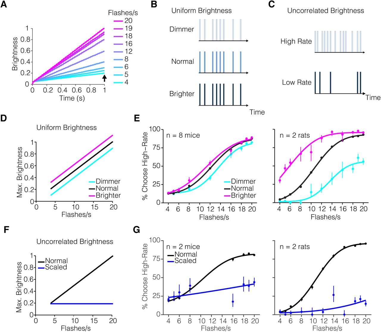
An alternate strategy to solve the visual pulses task is to accumulate photons or brightness over time, such that the decision is based on the overall brightness. This is a feasible strategy given that the flash event rate is directly proportional to the total LED on-time and therefore the total photons emitted in a sequence (Figure 4A, Supplementary Figure 2).

– (A) Schematic of simulated cumulative brightness across time for individual flash rates. Simulated brightness curves computed as the cumulative sum of the flash sequence for a given flash rate. Each curve represents an average (of n=250 trials) of a given flash rate. (B) Schematic of uniform brightness manipulation experiment. The intensity of individual flashes was varied such that all flashes appeared dimmer or brighter than normal. (C) Schematic of uncorrelated brightness manipulation experiment. The intensity of individual flashes was scaled inversely with the flash rate. (D) Schematic of cumulative brightness for each sequence (arrow in panel A), plotted against flash rate in uniform brightness manipulation experiment. (E) Psychometric performance on uniform brightness manipulation experiment: mice (n = 8) and rats (n=2). Subjects were presented with brighter (magenta) or dimmer (cyan) pulse sequences randomly on 5% of all trials. (F) Schematic of cumulative brightness for each sequence (arrow in panel A) plotted against flash rate for uncorrelated brightness manipulation experiment. In contrast to normal sequences (black), the scaled sequences have the same cumulative brightness, independent of their flash-rate (blue). (G) Psychometric performance from uncorrelated brightness perturbation experiment: mice (n = 2) and rats (n = 2). Subjects were presented with brightness scaled pulse sequences randomly on 5% of all trials. Circles represent subjects’ behavioral responses. Solid line represents 4-parameter cumulative Normal psychometric function fit to the data. Error bars represent Wilson binomial 95% confidence intervals.
To test whether rodent subjects performing the visual pulses task were sensitive to changes in brightness, we performed two brightness manipulation experiments. First, the intensity of all flashes in a given sequence was randomly increased on decreased on 5% of all trials (Figure 4B). If subjects are influenced by brightness, they will tend to report more high-rate choices on trials with brighter pulse sequences, and on dimmer trials report low-rate choices (Figure 4D). For comparison, we also tested rats on the same manipulation. Brightness influenced the decisions of both mice and rats (Figure 4E). For mice, changes in brightness had a modest effect on the psychometric performance whereas rats were more sensitive to the brightness perturbation.
Second, we remove the correlation between brightness and flash rate by adjusting the flash intensity in each sequence to the flash rate. As a result, the total brightness over time was the same across all flash rates (Figure 4C,F). If subjects were invariant to the total brightness of a sequence, and instead relied on flash count, this manipulation should not interfere with their performance. However, performance on the scaled brightness trials (5% of all trials) was dramatically changed (Figure 4G): both mice and rats chose the low-rate port on almost all trials. Because the overall brightness for each flash rate was made equal to that of a typical extreme low-rate stimulus (i.e. 4 flashes/s), low rate choices may reflect that animals based choices only on brightness. An alternative interpretation is that the reduced brightness increased uncertainty of the animals (Sheppard et al. 2013), leading to an overall loss of sensitivity and thus a flat psychometric function. In keeping with this possibility, note that mice chose the high rate option more frequently at the very lowest rates on the scaled trials compared to the normal trials (Figure 4G, left). Had they used solely a brightness strategy, they would have chosen the high rate option less frequently for those trials. Although more experiments are needed to fully understand how brightness and count are weighted during decision-making, these results make clear that the decisions here were not based solely on count. This suggests that future experiments should train animals to marginalize over brightness, perhaps by using stimuli with variable brightness from the onset of training.
Inactivation of secondary visual area AM biases perceptual decisions
To test whether the evidence accumulation paradigm engaged cortical circuitry, we sought to reversibly silence secondary visual AM in mice performing the task. We performed widefield retinotopic mapping in each mouse to identify AM for targeted inactivation (Figure 5). Briefly, we imaged visually evoked activity in awake transgenic mice expressing GCaMP6 in excitatory neurons (Ai93; CamkIIα-tTA; Emx-cre) in response to a vertical or horizontal bar that periodically drifted across the screen in the four cardinal direction (Kalatsky and Stryker 2003; Garret et al. 2014; Zhuang et al. 2017). This procedure enabled generation of phase maps for altitude and azimuth visual space (Figure 5A, B) and subsequently visual field sign maps (Figure 5C), which were used to estimate the borders between cortical visual areas and reliably identify visual AM (Figure 5D). To reversibly silence AM, we used cruxhalorhodopsin JAWS (Halo57), a red light-driven chloride ion pump capable of powerful optogenetic inhibition (Chuong et al. 2014; Acker et al. 2016). Optogenetic stimulation was randomly interleaved in 25% of all trials within a session. The optogenetic stimulus pattern consisted of a 1 s long square wave followed by a 0.25 s long linear downward ramp to reduce the effect of rebound excitation that may occur after strong inhibition (Figure 6A) (Chuong et al. 2014; Guo et al. 2014a).
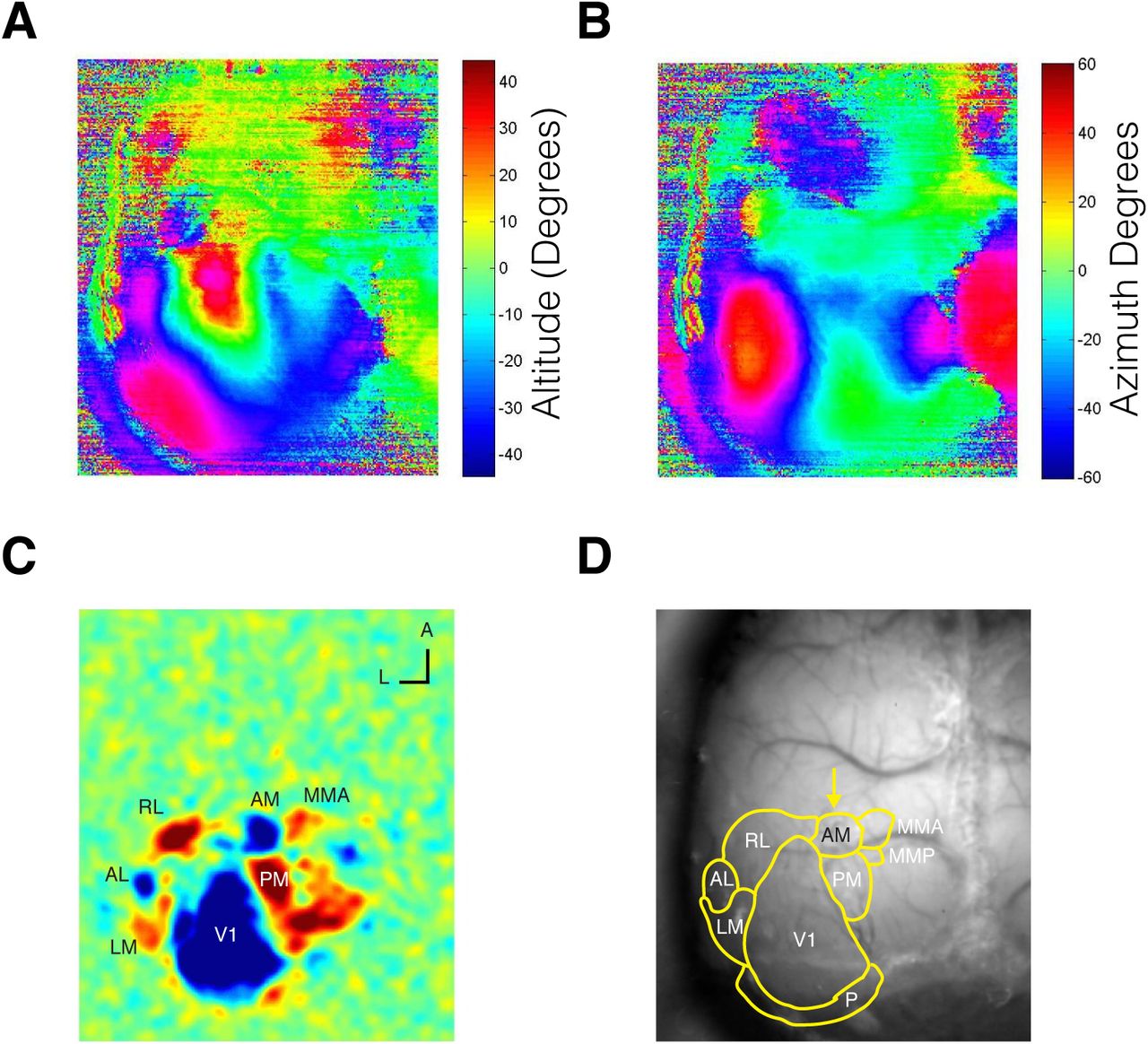
(A) Altitude and (B) azimuth phase maps (C) Visual field sign map with labeled visual areas (D) Visual area borders overlaid on photograph of skull.

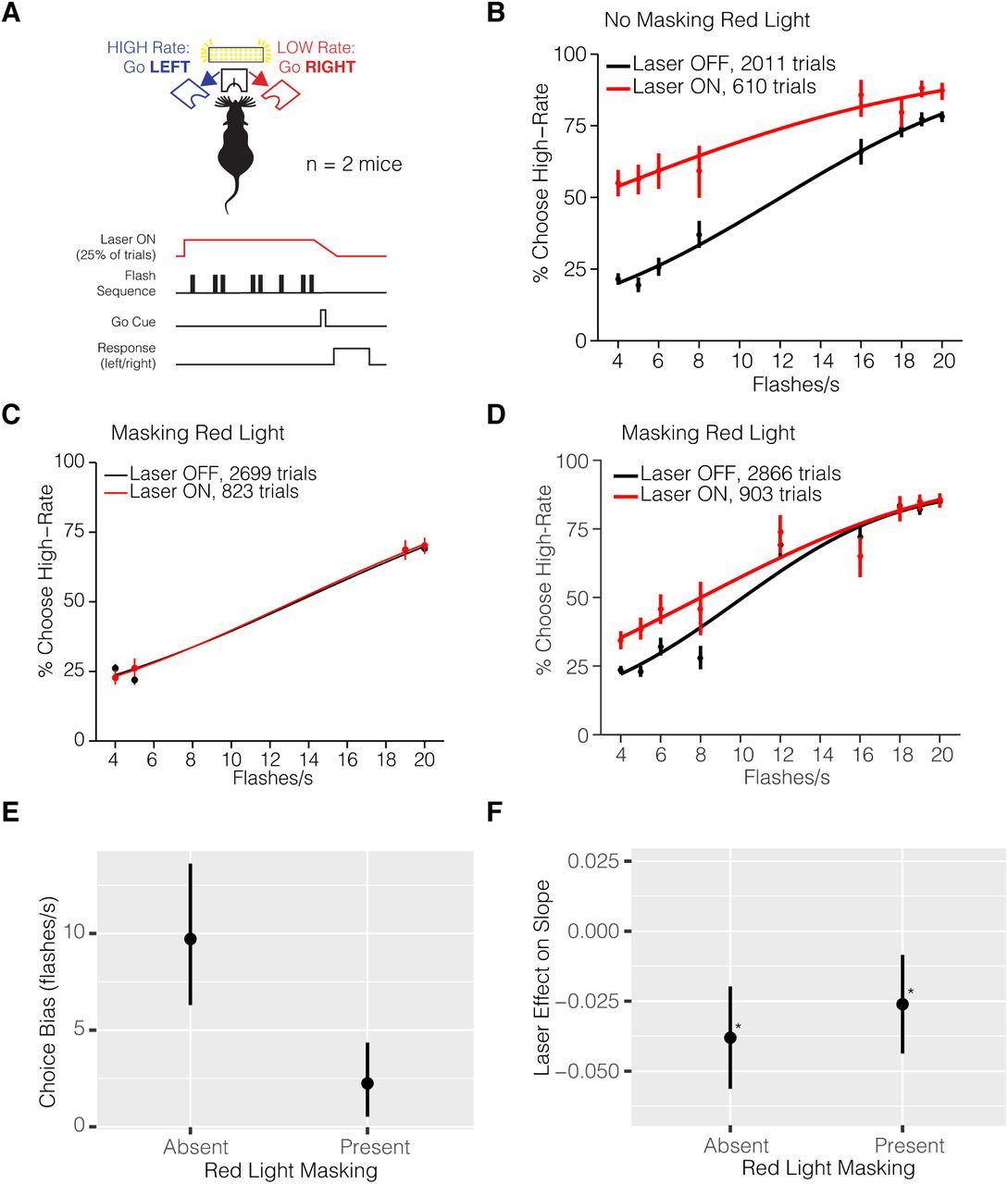
(A) Experimental configuration of control group. Mice were injected with AAV-GFP and implanted with a fiber in right hemisphere area AM. (B) Psychometric function of control group mice (n = 2) without masking red light. Irradiance at 32 mW/mm2. Psychometric performance of control group mice (n = 2) with masking red light (C) with easiest flash rate conditions and (D) multiple flash rates. Irradiance at 64 mW/mm2. Psychophysical effects of in vivo red light stimulation on the (E) the estimated choice bias and (F) the slope of the psychometric function (βevidence:opto) in the presence or absence of masking red light. Irradiance for masking light ‘Absent’ condition is 32 mW/mm2 and 64 mW/mm2 ‘Present’ condition.
A potential confound when using JAWS for optogenetic inhibition is a behavioral artifact due to the presence of visible red light. While it was long assumed that rodents are unable to perceive red light, a recent study showed that red-light delivery in the brain can activate the retina and influence behavior (Danskin et al. 2015). If mice are influenced by brightness in their decisions (Figure 4), red-light stimulation could induce a behavioral bias towards high-rate decisions during photoinhibition trials. In addition, decisions could be biased towards the location of the optical fiber. To test whether mouse behavior would be affected by the presence of red light in the absence of JAWS we implanted and trained mice injected with a sham virus (AAV-GFP) in AM.
In vivo red light stimulation of the control group resulted in a bias towards the high-rate side (Figure 6) confirming the hypothesis that the red light alone introduces an artifact in the behavior, most likely due to red light directly exciting the retina and increasing the perceived cumulative sequence brightness. To eliminate this behavioral artifact, we installed additional red lights in the behavior booth to adapt long-wave sensitive photoreceptors in the retina (Danskin et al. 2015). The external house red lights strongly reduced the animals’ red-light sensitivity during photoinhibition trials (Figure 6C-E).
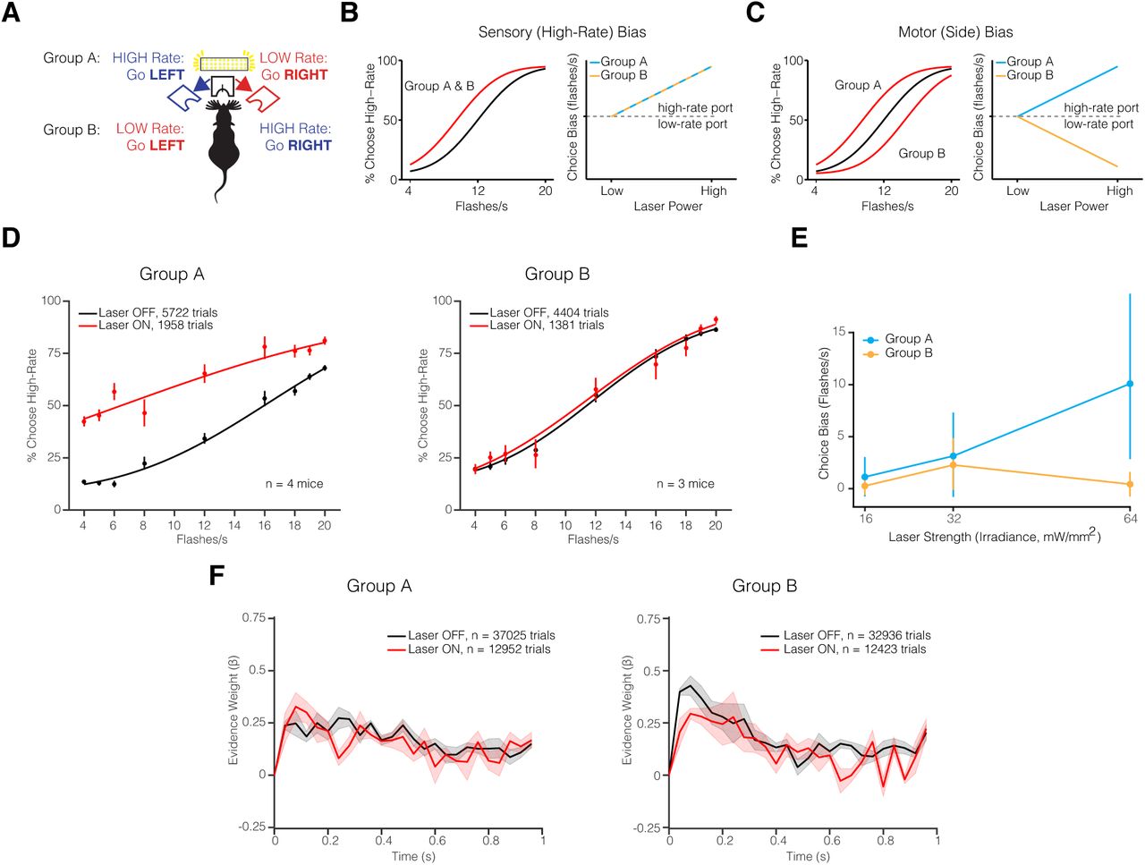
Having established that the red light alone will influence behavior, we developed an experimental design in which the stimulus-response contingency was varied while the stimulated hemisphere was held constant. This allowed us to distinguish between a potential spatial/motor and a sensory bias due to unilateral inhibition of AM. We trained two groups of mice on opposing behavioral contingencies: the first group (A) trained on the contingency: High-Rate, go LEFT and the second group (B) trained on the reverse contingency: High-Rate, go RIGHT (Figure 7A). Comparing these two groups allowed us to disentangle whether an observed bias is due to unilateral inhibition of AM and if the bias is sensory or spatial-motor in nature. If AM inhibition causes a sensory bias (e.g. towards the high-rate stimulus) both groups should exhibit a leftward shift in the psychometric function (Figure 7B). However, if AM inhibition causes a spatial-motor bias towards the ipsilateral hemifield, then the psychometric function for the two groups would shift in the opposing directions (Figure 7C) such that Group A exhibits a leftward shift and Group B a rightward in the psychometric function. This difference can be further quantified by the choice bias measure as a function of laser power strength. A positive choice bias indicates a bias towards the high-rate choice port and therefore a leftward shift in the psychometric function, whereas a negative choice bias value indicates a bias towards the low-rate port and a rightward shift in the psychometric function.

– (A) Schematic of experimental configuration of AM photoinhibition experiment. Group A (n =4) mice trained on the contingency: High-Rate, go LEFT and Group B mice trained on the reverse contingency: High-Rate, go RIGHT. Both groups of mice were injected with JAWS virus and implanted with an optical fiber implanted on the left hemisphere. Photoinhibition occurred on 25% of trials during the stimulus period. (B, C) Predicted behavioral outcomes of AM photoinhibition: AM inhibition could cause (B) sensory bias towards high rate stimulus or (C) motor (side) bias towards the ipsilateral hemifield. (D) Psychometric performance fits of group A and B mice. Mice performed the task with masking red light installed in the behavior booth and laser power irradiance of 64mW/mm2. Circles represent the subject’s behavioral response during laser OFF (black) and laser ON (red) trials. Solid line represents the psychometric function fit to cumulative Normal. Error bars represent Wilson binomial (95%) confidence intervals. (E) Estimated choice bias as a function of irradiance. (F) Psychophysical kernels pooled separately across mice in groups A and B.
Mice from group A (High-Rate, go LEFT) exhibited pronounced impairment in psychophysical performance across multiple tested laser power (irradiance) levels (Supplementary Figure 4). Inhibition of AM caused a consistent leftward shift in the psychometric function of group A mice with increasing laser strength (Figure 7D, E and Supplementary Figure 4) and significantly reduced the slope of the psychometric functions at irradiance levels of 32 mW/mm2 (p = 7.2e-05, GLMM Test) and 64 mW/mm2 (p = 3.4e-06, GLMM Test) (Supplementary Figure 5). In mice from group B, the psychometric function exhibited a leftward shift at 32 mW/mm2 (Figure 7D and Supplementary Figure 4), but not at 64 mW/mm2 (Figure 7E). If both groups of animals experienced a sensory high-rate bias, then their choice biases should increase with photoinhibition strength (Figure 7B). However, this relationship was only observed in the group A, but not group B mice (Figure 7E).
A potential explanation for these differences is that photoinhibition of AM causes a bias towards the ipsilateral hemisphere. Our hypothesis is that the ipsilateral bias effect is combined with the residual high-rate artifact caused by in vivo red light stimulation that we demonstrated using uninjected controls (Figure 6). In group A, the photoinhibition site (left hemisphere) and high-rate (left hemifield) choice port are congruent, a choice bias due to AM inhibition and a red light artifact would therefore sum to produce the observed strong high-rate bias. In group B, the photoinhibition site (left hemisphere) and high-rate choice port (right hemifield) are in opposition: a choice bias due to AM inhibition and a red light induced, high-rate artifact would therefore compete, and partially cancel each other out. Consistent with this hypothesis, at 64 mW/mm2 irradiance, group B mice exhibited no change in choice bias or the sensitivity. However at 32 mW/mm2 the choice bias tends toward positive, and may be a result of the residual red light artifact, which outweighs the ipsilateral choice bias caused by AM inhibition.
Discussion
We report a quantitative behavioral paradigm for studying visual evidence accumulation behavior of freely behaving mice. Mice trained on our paradigm performed several hundreds of trials per session and maintained stable performance across sessions. Similar to previous perceptual decision making studies in humans (Abrahamyan et al., 2016; Urai et al., 2017) and rats (Scott et al., 2015), mice trained on our task were influenced by previous reward and choice history. In addition, we demonstrated that area AM plays a causal role in visual decisions. Our strategic experimental design was key in allowing this conclusion because control experiments demonstrated that the red stimulation light biases mice even in the absence of JAWS.
Mice trained on this task deviated from an ideal integration strategy, and instead assigned more weight on average to flashes presented earlier in the sequence. This observation is consistent with results from the evidence accumulation paradigm from Morcos and Harvey (2016) in head-fixed mice. Further, the shapes of the psychophysical kernels we observed in the mice are qualitatively similar to those observed in nonhuman primates (Katz et al. 2016; Yates et al. 2017). Interestingly, the shape of the kernel differed from those observed in rats trained on the same task (Figure 2B) and previously reported by other evidence accumulation paradigms (see Raposo et al. 2012; Brunton et al. 2013; Scott et al. 2015). The difference in psychophysical weighing of evidence across species is intriguing because it suggests that although different species achieve comparable levels of performance on the same task, their internal behavioral strategies may differ. This underscores the importance of using stochastic stimuli, which make it possible to uncover the animal’s strategy (Churchland and Kiani 2016).
The brightness manipulations revealed that perceptual decisions on our task were affected by the brightness of individual flashes. While the results do not rule out that rodents are incapable of using a counting strategy, our experiments demonstrate that for both mice and rats, the cumulative brightness of the flash sequence influenced their decision. The susceptibility of the rats to the brightness perturbations is in contrast to findings from a recent study, which reported that rats performing a visual evidence accumulation task counted individual flashes rather than cumulative brightness (Scott et al., 2015). Though the authors manipulated brightness by randomly varying the duration of flashes, their manipulation preserved the correlation between cumulative brightness and flash count similar to our uniform brightness manipulation (Figure 4B). We found the strongest effect of cumulative brightness perturbation when we removed the correlation between the cumulative brightness of a sequence and the flash count. Further experiments are needed to explore whether rodents can be trained on such a stimulus.
To understand the neural mechanisms that enable perceptual decision making, we tested the causal involvement of secondary visual AM for behavior. Our results suggest that AM is involved in guiding contralateral choice behavior. More work is needed to resolve the role of AM, as the results are potentially confounded by the presence of red light during photoinhibition. Nevertheless, we demonstrated for the first time that a secondary visual area in the mouse contributes to decision making behavior that requires evidence accumulation. These experiments lay the groundwork for further investigations of the neural circuits that underlie evidence accumulation of visual evidence across time in the mouse. Future experiments should focus on using the tools available in mouse to characterize the nature of the neural signals underlying evidence accumulation as well as how this signal influences downstream processes to direct behavior.
Implications of AM photoinhibition
The red light artifact makes it difficult to precisely disentangle the true nature of the effect of AM photoinhibition. The artifact was greatly reduced, although not eliminated, by training the mice with house red lights (Figure 6). The artifact is most likely caused by red light propagating from the stimulation site through the brain and directly activating the retina (Danskin et al. 2015). The additional red light produces an apparent increase in overall brightness, which is positively correlated with the high-rate flashes (Figure 4A). Danskin et al. (2015) measured retinal activation during in vivo red light stimulation and found the largest activation ipsilateral to the implanted stimulation fiber. This could imply that mice would have an increased tendency to go towards the hemifield ipsilateral to the implanted fiber. Since the visual flashes stimulus is non-spatial, it is unlikely that mice are directly biased towards the implant site. Instead, the behavioral artifact of red light stimulation appears to arise from a cumulative brightness strategy that mice use to solve the task.
The proposed ipsilateral bias caused by AM photoinhibition is consistent with spatial hemineglect observed in visual parietal lesions. Spatial hemineglect, also referred to as contralateral neglect, is a phenomenon that occurs when subjects ignore the contralateral hemifield as a result of lesion to the parietal cortex. Although hemineglect has been reported in humans (Stone et al. 1991; Kerkho 2001) and rats (Crowne et al. 1986; Reep and Corwin 2009), we could not find a report on mice. The presence of hemispatial neglect would suggest that the mice are neglecting the tendency to go towards the affected (contralateral) visual hemifield. A related interpretation of the ipsilateral bias due to suppression of AM activity is that neurons in AM represent the intent to make contralateral choices. Intention, in the neuroscience literature, is defined as an early plan for movement, which specifies the goal and type of movement (Andersen and Buneo 2002). Under the intention scenario, the two hemispheres of AM would represent competing movement intentions, such that inactivation of one hemisphere leads to movement in the opposing direction.
In summary, our results support a role for AM in visually guided evidence accumulation behavior. We propose that AM drives contralateral choices in the visual flashes task, such that AM inhibition leads to an ipsilateral side bias. This is consistent with anatomical projections of AM to motor areas (Supplementary Figure 3) and the recently proposed role for mouse parietal cortex in navigation (Krumin et al. 2017). Applied to our task, AM, which belongs to the mouse parietal cortex, likely encodes the navigational (or spatial) signals of where the mouse should go given the flash rate. Further efforts are required to firmly establish these findings and its generalization to other visually guided tasks in the mouse.
Materials and Methods
Animal Subjects
The Cold Spring Harbor Laboratory Animal Care and Use Committee approved all animal procedures and experiments. Experiments were conducted with female or male mice between the ages of 6-25 weeks. All mouse strains were of C57BL/6J background and purchased from Jackson Laboratory. Ten GCaMP6f transgenic mice (Ai93 /Emx1-cre /CamKIIα-tTA) of both sexes were used for retinotopic mapping and area AM photoinhibition experiments. Four male Long Evan rats (6 weeks, Taconic) were also used for behavior experiments.
Behavioral Training
Before behavioral training, mice were gradually water restricted over the course of a week. Mice were weighed daily and checked for signs of dehydration throughout training period (Guo et al. 2014b). Mice that weighed less than 80% of their original pre-training weight were supplemented with additional water. Behavioral training sessions typically lasted 1-2 hours, daily, in which mice typically harvested at least 1 mL of water. Mice rested on the weekends. If a mouse failed to harvest at least 0.4 mL on two consecutive days, the mouse was supplemented with additional water.
Animal training took place in sound isolation chamber, which contained a three-choice port box. The mouse would poke into the center port to initiate trials and deliver the stimulus. Given the stimulus, the animal reported its choice on either the left-or right-side port. In the first training stage, mice learned to wait for at least 1100 ms at the center port before reporting their decision. We shaped the behavior by rewarding the mice at the center port (0.5 μL) and gradually increasing the minimum wait duration from 25 ms to 1100 ms over the course of 1-2 behavioral sessions. Without center reward, this stage typically took 10-12 sessions to learn.
During the first stage, mice were not rewarded for making the correct association between the stimulus and response port; rather on each trial, a random port (left or right) was chosen as the reward port and a liquid reward (2 to 4μL) was delivered to the port. Trials in which the mouse waited the minimum required duration at the center port are referred to as completed trials. In our initial training procedure, it took mice 10 to 12 session to learn to wait at least 1000 ms (Supplementary Figure 1G). However, delivering a small liquid reward at the center port (0.5 μL) significantly reduced the time it took mice to learn to wait at the center and increased their trial completion rates (Supplementary Figure 1H,J). Mice rewarded at the center port achieved a completion rate above 90% compared to mice not rewarded at the center port.
In the second stage of training mice were trained to associate high-rate flashes sequences (>12 flashes/s) with the right-hand port and low-rate flashes (< 12 flashes/s) with the left-hand port. Trials with flash rates of 12 flashes/s were randomly rewarded on the left or right side port. For some mice, the contingency was reversed, such that high-rate flashes were rewarded at the left-hand port and low-rate flashes were rewarded at the right-hand port. Mice were rewarded for correct and punished for incorrect responses or withdrawing with a time-out period (2 to 4 s), during which the mouse was not allowed to initiate a trial. Trials with flash rates equal to 12 flashes/s were randomly rewarded on the left or right side port.
We employed several anti-bias methods to correct the side bias, which often occurred when mice began stage two. A few examples of anti-bias strategies include physically obstructing access to the biased port, changing the reward size, or proportion of left vs. right trials. A mouse was considered trained once they are unbiased, performing above chance, and experiencing all stimulus strengths. Trial type, stimulus and reward delivery, control, and data collection was performed through a MATLAB interface and Arduino-powered device called BPod (SanWorks LLC).
Stimulus Generation
The stimulus consists of a sequence of 20 ms pulses of light from a LED panel (Ala Scientific). The inter-pulse intervals are randomized from a discrete exponential distribution. For the exponential interval stimulus, the minimum inter-pulse interval was 20 ms, and the number of flashes for a given stimulus determined the maximum interval. The number of flashes was between 4-20 flashes/s. The stimulus was created using 25 fixed time bins each 20ms in duration. A Poisson coin was flipped to determine whether an event (flash) would occur in each bin. An empty 20ms time bin followed each fixed time bin.
Brightness Manipulation
For the brightness manipulation experiments, we wanted to keep the flash duration of 20ms constant, so that the subjects could not use the flash duration as a cue for the correct stimulus category. Each 20ms flash pulse was generated by a half-wave rectified sinusoidal signal thresholded at the peaks and with a base frequency of 200Hz. This approach effectively controls the total LED ON time or the “density” of the 20ms pulses. It is similar to pulse-width modulation technique used to control LED brightness. During normal sessions, the base frequency is multiplied by a brightness factor, which is kept constant across sessions. In the uniform brightness manipulation experiment, the normal brightness factor was either halved or doubled on 5% of trials to produce the “dimmer” and “brighter” conditions. In the uncorrelated brightness manipulation experiment, we varied the LED on time within the flash duration such that the normal brightness factor was inversely scaled with the flash rate. Because the lowest number of flashes presented was 4 flashes/s and we chose not to change the flash duration, we normalized all flash sequences such that the total LED on time was equal to 4 flashes/s. All brightness manipulations were randomly introduced on 5% of all trials.
Head bar implantation and skull preparation
For retinotopic mapping experiments, mice were implanted with a custom titanium head bar. Mice were anesthetized with isoflurane (2%) mixed with oxygen and secured onto a stereotaxic apparatus. Body temperature was maintained at 37 °C with a rectal temperature probe. The eyes were lubricated with eye ointment before the start of the surgery, followed by subcutaneous injection of analgesia (Meloxicam, 2mg/kg) and antibiotic (Enrofloxacin, 2mg/kg). Fur on the scalp was removed with hair clippers and Nair (Sensitive Formula with Green Tea), followed by betadine (5%) swab. Lidocaine (100 μL) was injected underneath the scalp before removing the scalp. The skull was cleaned with saline and allowed to dry. A generous amount of Vetbond tissue glue (3M) was then applied to seal the skull. Once the Vetbond was dry, the head bar was secured with Metabond (Parkwell) and dental acrylic. Mice were allowed 3 days to recover before retinotopic mapping.
Retinotopic Mapping
Retinotopic mapping was performed in awake head-fixed animals adapted from (Garrett et al, 2014; Juavinett et al. 2016). For periodic (Fourier) stimulation, a narrow bar (10°) was drifted across the four cardinal directions of the screen. Presented within the drifting bar was a flickering checkerboard pattern (12° checks, 5Hz). One trial consisted of 11 sweeps of the bar in 22 seconds in one of the four cardinal directions, however the first cycle was discarded because it typically introduced stimulus onset transients. Each trial was repeated 15 times for each direction. The monitor was placed in contralateral visual hemifield to imaging hemisphere, positioned at an angle of 77° from the midline of the mouse and a distance of 15 cm. Imaging data was acquired at 20 frames per second.
Optogenetic Inactivation
For JAWS inhibition experiments, mice were injected with AAV8-CamKII-JAWS-KGC-GFP-ER2 into area AM identified by retinotopic mapping. Virus injections were performed using Drummond Nanoject III, which enables automated delivery of small volumes of virus. To minimize virus spread, the Nanoject was programmed to inject slowly: six 30 nL boluses, 60 s apart, and each bolus delivered at 10 nL/sec. Approximately 180nL of virus was injected at multiple depths (200 and 500 μm) below the brain surface. Following the virus injection, 200 μm fiber (metal ferrule, ThorLabs) was implanted above the injection site. The optical fiber was secured onto the skull with Vitrebond, Metabond, and dental acrylic. The animals were allowed at least 3 days to recover before behavioral training. A red 640nm fiber-coupled laser (OptoEngine) was used for inactivation. Experiments were conducted with multiple laser power levels: 0.5, 1, and 2 mW (16, 32, and 64 mW/mm2). One power level was used per session. On inactivation sessions, laser light was externally triggered using a PulsePal (Sanworks LLC) device. The laser stimulation pattern was a square pulse (1 second long) followed by a linear ramp (0.25s), which began at the onset of the stimulus. Stimulation occurred on 25% of trials.
Psychometric function
We fitted a four-parameter psychometric function to the responses of subjects that performed the visual flashes categorization task. The general form of the psychometric function defines the probability (pH) that the subject chooses the port associated with high flash rate as:

γ and λ are the lower and upper asymptote of the psychometric function, which parameterize the guess rate and lapse rate, respectively; F is a sigmoidal function, in our case a cumulative Normal distribution; x is the event rate i.e. the number of flashes presented during the one second stimulus period; β parameterizes the horizontal shift or bias of the psychometric function and α describes the slope or inverse sensitivity. The psychometric function F(x; α, β) for a cumulative Normal distribution is defined as:

The parameters of the psychometric function were estimated with the Palamedes Toolbox (Prins and Kingdom 2009).
Choice History
We implemented two choice history models to evaluate the influence of prior choice(s) on the current choice of the subject. The first approach, assessed whether success or failure on the most recent trial influenced the performance on the current trial (Busse et al. 2011):
 t indicates the current trial and E is the signed stimulus evidence of the current trial. Evidence is computed as the difference between the flash rate of the trial and the category boundary (12 flashes/s). Isuccess and Ifailure are indicator variables for success (reward) and failure on the previous trial, respectively. The coefficients (β0, βE, βS, βF) were estimated with MATLAB glmfit.
The second approach used was a probabilistic model described by (Fründ et al 2014):
 t indicates the current trial and E is the signed stimulus evidence of the current trial. The additional regressors Eτ and Cτ represent the evidence and choice on τ previous trials in the past, respectively. Coefficients (β0, βE, βE(τ),and βC(τ)) were estimated with MATLAB glmfit.
Logistic Regression Reverse Correlation
The logistic regression function for estimating the weights associated with each moment of the stimulus can be written as:
 pH is the probability of choosing the high-rate port, I is an indicator variable for whether or not a flash pulse occurred in time bin i, and N is the number of time bins. The coefficients β0… βN are estimated with the MATLAB function glmfit.
Generalized Linear Mixed Model (GLMM)
To statistically test whether there was a significant effect of photoinhibition of area AM on the population group level, we used a Generalized Linear Mixed-Model (GLMM). GLMMs are an extension of the Generalized Linear Model, which can be used to model both fixed and random effects in categorical data. In psychophysics, GLMMs can be used to generalize results across multiple subjects and experimental conditions (Knoblach and Maloney 2012; Moscatelli et al. 2012; Erlich et al. 2015).
The GLMM model written in the Wilkinson notation:

Each term of the equation has a coefficient, β. The model specifies that the subject’s response, r, is a function of the fixed effects: intercept, the evidence, which represents the slope of the psychometric function and is defined as the difference between the flash rate and the category boundary, the photoinhibition indicator variable opto, and the interaction between the evidence and opto. The interaction term evidence:opto evaluates whether photoinhibition alters the subject’s sensitivity or the slope of the psychometric function. The model allows the four fixed effects parameters to vary for each individual subject (random effects). The model uses a probit linking function and was fit using a Maximum Likelihood procedure. The GLMM analysis was performed using the R package ’lme4’ similar to Erlich et al (2015).
The effect of photoinhibition on the horizontal location of the psychometric function was quantified by the choice bias. The choice bias was defined as:
 βopto, βevidence, βevidence:opto are estimated coefficients from the GLMM equation above. The choice bias reflects the equivalent change in the stimulus that would recapitulate the observed effects of photoinhibition and is in units of flashes/s. Positive choice bias would indicate that on photoinhibition trials caused the subject to be biased towards high-rate responses. Since the choice bias is computed from estimated parameters of the GLMM model, we computed the errors (95% confidence intervals) via error propagation.
Author Contribution
Conceptualization, O.O. and A.K.C; Methodology, O.O., H.N, and A.K.C; Software, O.O.; Formal Analysis, O.O.; Writing – Original Draft, O.O.; Writing – Review & Editing, A.K.C.; Funding Acquisition, O.O. and A.K.C; Investigation, O.O. and H.N; Visualization, O.O. and A.K.C.; Resources and Supervision, A.K.C.
Acknowledgements
We thank Rob Eifert and Barry Burbach for technical support. We thank Sashank Pisupati, Simon Musall, Matthew Kaufman, Ashley Juavinett, and Lindsey Glickfeld for helpful discussions and feedback on the manuscript. This work was supported by NIH NRSA F31 (1F31-EY025164) to O.O, The Simons Collaboration on the Global Brain, The Klingenstein Foundation and the Pew Charitable Trust to A.K.C.


