

Abstract
Reconstruction of neural circuits from volume electron microscopy data requires the tracing of complete cells including all their neurites. Automated approaches have been developed to perform the tracing, but without costly human proofreading their error rates are too high to obtain reliable circuit diagrams. We present a method for automated segmentation that, like the majority of previous efforts, employs convolutional neural networks, but contains in addition a recurrent pathway that allows the iterative optimization and extension of the reconstructed shape of individual neural processes. We used this technique, which we call flood-filling networks, to trace neurons in a data set obtained by serial block-face electron microscopy from a male zebra finch brain. Our method achieved a mean error-free neurite path length of 1.1 mm, an order of magnitude better than previously published approaches applied to the same dataset. Only 4 mergers were observed in a neurite test set of 97 mm path length.
Introduction
Computers have been employed for the reconstruction of neural ‘wires’ since the 1970s 1mainly to capture and display the annotation decisions made by human tracers 2–4. The use of computers to make those decisions based on algorithms designed to detect the boundaries of cells began in earnest after new and improved approaches to the acquisition of volume EM data 5 started producing datasets for which the complete analysis by human annotation would be prohibitively expensive. It quickly became clear that machine learning approaches, now mostly based on convolutional neural networks (CNNs), are the method of choice 6. While those algorithms find most cell boundaries, the remaining error rates required the use of human proofreading, which could either take the form of inspecting the fragments (supervoxels) of an oversegmentation generated by the algorithm 7or by creating skeleton tracings, which then are used to gather the fragments belonging to the same cell 8–10.
Unfortunately, human proofreading is prohibitively expensive for larger datasets. The estimated human labor required to reconstruct a 1003 μm3 volume exceeds 100,000 hours, even when using an optimized pipeline that combines automated neural network inference and manual skeletonization 11. Current manual annotation workflows could be made more efficient still but are ultimately limited by the need to view all the data. A reduction of the proof-reading time by multiple orders of magnitude requires algorithms that are not only substantially more accurate but also “know their own limits” and provide a list of potentially erroneous segmentation decisions. Humans would then have to inspect only those locations 12.
State-of-the-art automated neurite reconstruction generally is performed in two stages. First a convolutional network infers for each image location the likelihood of there being a boundary, using the intensities of the voxels at and near that location 13,14. A separate algorithm (e.g., watershed, connected components, or a graph cut approach) subsequently uses the boundary map to cluster all non-boundary voxels into distinct segments 11,15–18. We merged the two steps by adding to the boundary classifier a second input channel, which carries the predicted object map, leading to a recurrent model. Why is this helpful? While the cost function we used to train the network is still based purely on a voxel-wise comparison with the training set, the network can now learn to make use of the fact that certain voxels in its field of view (FoV) have already been classified with high certainty in an earlier iteration. Classification decisions can be based on, for example, whether those predictions result in a more or less plausible shape for the neural process. Shape information is thus incorporated in as much as it helps the network to improve its ability to predict the boundary map. Note that this is conceptually quite different from other approaches that use cost functions that depend directly on segmentation performance 19,20. Here we present a realization of this concept, which we call Flood-Filling Networks (FFNs).
FFNs are trained to distinguish a single object (the foreground) from all other objects (the background). In contrast to prior machine learning-based segmentation methods 11,16,21–23, FFNs segment one object at a time. With each iteration the feedback pathway carries past segmentation decisions forward in time and spreads them in space. This enables the FFN, which has a relatively small direct FoV, to integrate information from far beyond its direct FoV. It also transforms the problem of single-shot classification into classification conditioned on prior predictions (i.e., classification results from nearby locations), which we believe to be a simpler problem (see Supplementary for experimental data confirming this intuition). This makes it possible for results in “easy”, unambiguous areas to inform segmentation in “hard”, more ambiguous regions.
In the following, we describe the core FFN algorithm, how FFNs can be used to reconstruct a large-scale EM volume, compare accuracy to previously published alternatives, and analyze the errors of the FFN reconstruction in detail. The quality of the fully automated segmentation obtained with FFNs is shown to far exceed previous approaches, and opens up the possibility of efficient analysis of volumes that have so far been intractable due to their size.
Results
Flood-filling network architecture, inference, and training
An FFN has two input channels, one for the 3D image data and another one for the current state of the “predicted object map” (POM). Using values between 0 and 1, the POM encodes for each voxel the algorithm’s estimate of whether the voxel belongs to the object currently being segmented. At each iteration of the network’s recurrent dynamics the POM is updated for all voxels in the network’s current FoV.
We generated single-voxel seeds at locations well away from the cell’s putative boundaries as detected by a simple edge filter, because we had observed that seeds placed near cell boundaries often cause neighboring objects to erroneously merge (Fig. 1a). When starting segmentation of a new object, the networks FoV is centered on the seed and the seed location’s POMs value is set to 0.95, with all other voxels set to 0.05. The values are offset from 1 and 0 to prevent the network from learning large internal weights and overfitting 24.

The segmentation pipeline. (a) Segmentation of a subvolume with an FFN. Top row (left to right): EM image data, local intensity gradient magnitude estimated with the Sobel-Feldman operator, Euclidean distance transform of the gradient magnitude with local peaks highlighted with white dots. The peaks are used as seed points for FFN inference. Bottom row: sequential segmentation of the subvolume with an FFN. The yellow cross-hair symbol indicates the seed point. (b) The flood-filling inference process for a single object. The red square indicates the location of the FoV in the EM data (left column) and the POM. Red lines with arrows indicate the flow of information to the inputs. Each iteration (row) consists of one forward pass of a convolutional network that receives as input both the image and the current state of the predicted object mask (POM). In the first row, the initialization of the POM is shown as specified by a single pixel (white square) within the network’s FoV (red square). Successive rows show successive iterations of FFN inference that incrementally contribute inference values to the POM while the network’s FoV moves throughout the image space. (c) Multi-seed consensus procedure. Top row: cross section through the data with the FFN segment seeded by A (left) and seeded by B (right). Note the merger between a glial fragment and a dendritic branch in the left panel. Bottom row: surface renderings of the segmentation after oversegmentation-consensus. (d) Multi-scale oversegmentation-consensus. Top row: segmentation from full resolution data (left) contains a merger between an axon and glial fragment, and the segmentation from data downsampled 2x in-plane (right) contains a merger between the same glial fragment and a dendritic branch. Bottom row: segmentation and surface rendering of multi-scale oversegmentation-consensus results in which both mergers are fixed. (e) Flood-filling agglomeration. Top row: (left) a split dendritic branch; the white square shows area of zoomed insets (right) in which FFN segmentation is started from points A (top) and B (bottom) sequentially. Bottom row: rendering of containing objects of points A and B, which are agglomerated due to satisfying mutual consistency criteria of FFN agglomeration (see text for details). The scale bars correspond to 1 μm.
The direct FoV (i.e those voxels that are directly affect the current FFN inference step) is relatively small (33×33×17 voxels, or 297 × 297 × 340 nm). Based on the inference results, the FoV may move to a new location or, alternatively, inference may terminate and generate a fixed segment from the POM (see Methods for details). Once a segment is completely fixed all seeds overlapping this segment are discarded and segmentation starts anew at one of the remaining seeds until none remain.
We applied FFNs to a 96×98×114 μm (10624 × 10880 × 5700 voxels) sized region of zebra finch brain that had been imaged with Serial Block-face Electron Microscopy 25 at a resolution of 9 × 9 × 20 nm. A small fraction (0.02%, 148M voxels, contained in 35 subvolumes of varying size that were distributed throughout the volume) of the data set was manually segmented by human annotators and used as ground truth to train the FFN.
At the core of the FFN is a multi-layer CNN. During each iteration step the POM values for multiple voxels are updated, in our case all voxels of the current FoV. During training the POM is first initialized by seeding a single-voxel in the center of the 49×49×25 voxel training example. A single iteration is then executed and its result is used to update the POM (Fig. 1b). The network weights are then adjusted via stochastic gradient descent using a per-voxel cross-entropy (logistic) loss 24. This procedure is repeated with the FoV position at a number of locations offset from the center by +/− 8 voxels (72 nm) laterally and +/− 4 voxels (80 nm) in z direction. In order to optimize the training procedure and remain consistent with the inference procedure, a FoV position was used only if the POM value of the new center voxel exceeded 0.9 immediately before the move. The order of moves was randomized.
Irregularity detection and automated tissue classification to prevent segmentation errors
Many of the FFN’s errors occur at data irregularities, such as cutting artifacts or alignment mistakes. While frequent enough to affect the overall error rate, such irregularities are too rare (affecting fewer than one voxel in a hundred) for the network to learn how to avoid them. Rather than enriching them in the training set, we decided to instead detect such irregularities in a separate process. When an irregularity was found we partitioned the neural process. While such partitions were mostly splits (errors in which two processes are erroneously disconnected from one another), many of those splits were later corrected at the agglomeration stage. Objects that were not reconnected in this way could be candidates for later human proofreading.
We also observed that the segmentation quality often declined near objects, such as somata or blood vessels, that were significantly larger than the cross sections of typical axons, dendrites and the FFN’s FoV. To address this we trained a separate CNN to detect blood vessel, cell body, neuropil, myelin, or out of bounds voxels and used these classifications to prevent the FFN from extending objects beyond the neuropil.
Hysteresis and approximate scale invariance in FFNs
FFN segmentation results were dependent on the placement of the initial seed and on the order in which objects were segmented. There were, for example, cases where a merger (two or more processes are erroneously connected to one another) was only created between two objects (A and B) when the segmentation order was A-B but not when it was B-A (“unidirectional mergers”).
This can be exploited to eliminate mergers while increasing the number of splits by only a small amount. Specifically, we compared a forward segmentation of the data with its backward segmentation, for which the the order of seeds was reversed and accepted all splits as real (which we call the oversegmentation-consensus), which means that only those mergers remained that occurred in both segmentations (Fig. 1c). Just as we used different initial seeds to build consensus analyses, we were similarly able to use analyses carried out on subsampled raw images, despite the FFNs not being explicitly trained to do so. Bidirectional mergers at full resolution often disappear completely or become unidirectional when inference is run at a reduced resolution, which we confirmed for data that were downsampled in-plane by factors of 2 or 4 and two-fold in the axial direction. Note that downsampling increases the FoV in physical space in these cases to, respectively, 594 × 594 × 340 and 1188 × 1188 × 680 nm.
We finally generated an oversegmentation-consensus using forward and reverse segmentations at the original and at down-sampled resolutions (see Fig. 1c,d and Online Methods for details). These procedures are conceptually similar to the process of ensembling in machine learning, i.e. combining the decisions of multiple different classifiers. Others have used the averaged predictions of the same classifier applied to modified versions of the raw image 18,26. In our case, the classifier was also kept constant, and variance was generated by changing the initial conditions and the scale of the image. These procedures increased the number of splits by a factor of only 2, but reduced the number of mergers by a factor of 82 (see also Fig. 3b,c for path length statistics).
FFN agglomeration
In order to reduce the number of splits, we agglomerated segments throughout the volume. Unlike previous automated agglomeration approaches, which involve training a classifier to score pairwise merge decisions 27 or predict a compatibility score between an agglomerated segmentation and the raw image 28, we instead used the FFN model itself to perform agglomeration.
To determine whether a pair of segments in spatial proximity are part of the same neurite, we extracted a small subvolume (about 1 μm3 in size) around the point of their closest approach. We then placed seeds in parts of the two objects inside the subvolume, at locations maximally distant from object boundaries, and performed two independent FFN inference runs, one for each of these seeds, while keeping the remaining objects fixed (Fig. 1e). If the resulting POMs overlapped to a high degree (using the intersection-over-union Jaccard index as a criterion), the objects were merged. This procedure takes advantage of the sensitivity of the FFN to the seed location and allows calibration of merge decisions by varying the threshold applied to the intersection-over-union value.
Large-scale FFN segmentation pipeline
We combined tissue masking, FFN inference, oversegmentation-consensus, and FFN agglomeration into a three-stage pipeline that was used to segment the entire volume.
Alignment. The sections within the volumetric dataset were precisely registered using elastic alignment 29, which, compared to a translation-only alignment, reduced the number of partitions introduced by the irregularity-detection procedure.
Cell-body segmentation. The parts of the volume corresponding to the interiors of cells bodies were segmented by running a FFN restricted to voxels labeled as being part of a cell body by the tissue-type classification, using seeds manually placed into all 454 somas in the volume (1 human hour was required for manual annotation, but this task could also be automated with 0.97 precision and 0.96 recall 30). Explicit handling of cell bodies was necessary due to the dramatically different spatial scale of cell bodies (average diameter 9 μm) and neuropil, which comprised the majority of training data for the FFN (average diameter 0.19 μm).
Neuropil segmentation and agglomeration. FFN inference was restricted to voxels labeled as neuropil by the tissue classifier, and five separate segmentations were generated and reconciled with oversegmentation-consensus. FFN agglomeration was used to merge neurites in the segmentation, which reduced the total rate of splits by 44% and increased the run length by 1149%.
Evaluation of large-scale segmentation accuracy
The most popular datasets for comparison and evaluation of computational methods for EM reconstruction are relatively small subvolumes of tissue that have been completely segmented by hand, i.e. each pixel in the subvolume has been assigned to an object 18,31. First we evaluated FFN and comparison methods on a 5 × 5 × 5 μm subvolume but found that the accuracy of the methods on this subvolume did not predict a method’s performance on the 5000-times larger complete volume (for example, the fraction of ground truth neurite annotations containing a merger in the CNN+GALA baseline segmentation method increased from 7.3% to 46.3%; see supplementary for details).
Thus in order to measure the accuracy of segmentation results over length scales comparable to the path length of neurons in the complete volume, we “skeletonized” individual neurons 8. Human annotators used KNOSSOS software (https://knossostool.org/) to manually annotate individual neuron structure as a set of nodes and edges forming an undirected tree. We created two non-overlapping sets of skeletons. The tuning set, which was used to optimize the hyper-parameters of the segmentation pipelines, contained 13.5 mm total neurite path length (of which 27% was axonal) distributed among 12 neurites with a 0.8 mm median path length. The test set, which was used solely for evaluation purposes, contained 97 mm total path length (34% axonal) across 50 neurons (2 mm median path length). We found that the skeletons contained eight mergers and 66 splits (mostly missed dendritic spines), even after human consensus generation based on multiple independent tracings. We corrected this by having two human experts (M.J., J.K.) examine every putative merger in the automated segmentations, and then fix the manual skeletons when they were deemed erroneous.
Based on overlap with the automated segmentation, each edge of the ground truth skeletons was classified as either correctly reconstructed in the segmentation, omitted, split, or part of a merged segment11,32. For example, if a segment within the automated reconstruction overlapped nodes from two different skeletons, then all edges overlapping that segment were counted as “merged.”
Only about 1.4% of the total path length in the imaged volume has been manually skeletonized. This allowed us to automatically detect all splits that occurred in the skeletonized neurites, but only those mergers that were with with other skeletonized neurites. This severely underestimates the number of mergers per cell. To correctly estimate the merger rate, we also (in addition to all automatically produced segments that contained nodes from more than one skeleton) classified a segment as containing a merger if it contained at least two skeleton nodes and if any part of the segment extended farther than 2.2 μm away from the skeleton to which that node belonged.
Finally, we calculated an “expected run length” (ERL) that measures the average error-free path length of neurites in the automated reconstruction. Even a single omission or split terminates the accumulation of run length; segments containing mergers do not contribute any run length at all. Note that such severe penalization of mergers is useful when optimizing an automated segmentation method since it reflects the difficulty involved in manually finding and correcting mergers when proofreading. However, when evaluating a proofread segmentation, which when combined with synaptic annotations 30 will yield the connections matrix, a different metric that more equally weights split and mergers will reflect the usefulness of the segmentation better. See Supplementary for full details of manual skeletonization, edge classifications, and run length calculation.
Our final reconstruction (FFN-c in Fig. 3) reached an ERL of 1.1 mm and contained only 4 mergers (Fig. 2). None of these mergers were between the ground truth skeletons, and we detected them with the heuristic procedure described above.
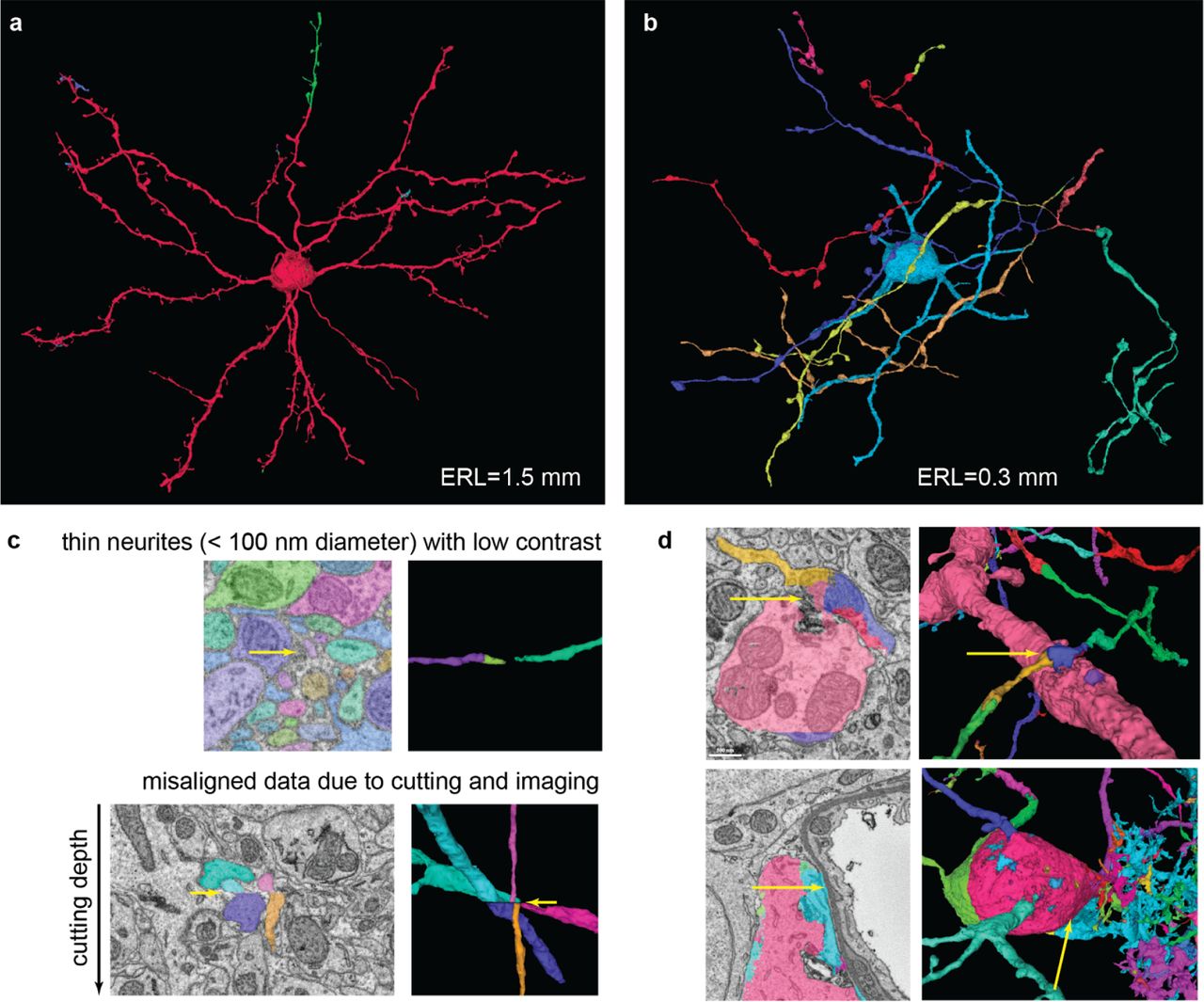
Qualitative analysis of segmentation accuracy. Different colors indicate different segments. Neurons reconstructed with the full pipeline (FFN-c) with (a) the largest (1.5 mm) and (b) shortest (0.3 mm) run lengths. (c) Zoomed views of splits caused by low contrast (top) and a slice misalignment (bottom). (d) Both rows show a set of pre-agglomeration segments (segments in FFN-b) that were erroneously merged during FFN agglomeration (segments in FFN-c). Top: dendrite-axon merger caused by small spillout of the dendrite segmentation. Bottom: cell body-glia merger caused by inaccurate cell body segmentation.

Segmentation method accuracies measured by comparison with 50 manually traced and verified skeletons (97 mm path length). SegEM: seeded watershed applied to convolutional neural network (CNN) boundary prediction 11, CNN: watershed over affinity graph predicted by a CNN, CNN+GALA: affinity graph watershed output agglomerated with a random forest classifier 27, FNN-a: single-pass FFN segmentation, FFN-b: FFN segmentation after multi-seed and multi-resolution consensus (note that the ERL decreased, but the merge rate is also decreased to almost 0), FFN-c: result of the entire FFN pipeline, including FFN agglomeration. (a) Expected run length. The end of the x-axis scale (at 2.1 mm) indicates the maximum ERL attainable for this dataset and set of ground truth skeletons. (b) Merger and split counts 11. (c) Fraction of ground truth skeleton edges classified as either split or merged. (d) Merge-free segment length distributions for the different segmentations. Error bars represent 95% confidence intervals and were calculated using the bootstrap method with 10,000 resamples.
To compare the performance of FFNs to alternative approaches to connectomic reconstruction, we implemented two of those approaches. The first approach, which we refer to as the “baseline,” combines a 3d convolutional neural network trained to produce long-range affinity graphs 21, affinity graph watershed segmentation 33, and random-forest object agglomeration using “GALA” 17,27. The convolutional network used an input FoV of 35×35×9 voxels and was trained to produce a long-range affinity graph that for every voxel predicted its binary connectivity to all its neighbors within a 3×3×1 radius. We also evaluated a recursive boundary prediction network 30 with a larger 201×201×21 FoV (for details of all network architectures see Supplementary), but found that it performed worse than the baseline network. The parameters for the affinity-graph watershed procedure were optimized by grid search, and GALA agglomeration was performed with a random forest classifier trained on the subvolumes of labeled data. Finally, we evaluated “SegEM” 11, in which 3d convolutional neural network boundary predictions are over-segmented with watershed. The same 3d convolutional network as the baseline was used, and we optimized the parameters by grid search over full volume segmentations. Among these alternative approaches, the baseline method achieved the highest ERL (112 microns; see Fig. 3 and Supplementary Table 5).
Analysis of errors by neurite type
We manually classified fragments of neurites in ground truth skeletons as axons or dendrites, and annotated the locations of the base and the head of 182 dendritic spines. We then used this data to measure error rates of the FFN-c segmentation for the different neurite categories (see Supplementary for details). We observed that the automated reconstruction is better than human annotators in identifying dendritic spines (95% and 91% recall, respectively). While precision remained close to 100% and was slightly higher for the automated results (99.7%, 100% automated vs 98%, 99% human-generated for dendrites and axons, respectively), recall for both axons and dendrites was still inferior to human performance (68%, 48% automated vs 89%, 85% human-generated for dendrites and axons, respectively).
Many of the remaining splits could be attributed to data artifacts, which affects all types of neurites, or low contrast (Fig. 2c), which affects only low-diameter processes such as axons. We attempted to correct for misalignment and single-slice artifacts in the agglomeration procedure (see Methods), but there remain difficult cases that, while unambiguous to humans, require further improvement in automated techniques.
Discussion
Flood-filling networks differ from other machine learning-based segmentation approaches in several ways: a recurrent network architecture, the direct generation of segments (rather than having to rely on a separate clustering step), and an inference procedure that segments objects one at a time. We also exploited several additional capabilities of FFNs, such as the ability to reduce mergers by ensembling multiple segmentations generated by varying seed point location. Applying these techniques to a roughly 1 million cubic micron volume of songbird tissue yielded automatically segmented neurons with an average error-free run length of 1.1 mm.
The main disadvantage of FFNs is the high computational cost. For example, performing a single pass of the fully-convolutional FFN network over the whole volume is 14.4x more expensive than the more traditional 3d convolution-pooling architecture in the baseline. This is because multiple and partially overlapping inference computations are required to segment both a single object as well as implement the sequential nature of multiple object segmentation. On average, every voxel of the volume was processed by the FFN 59 times in a segmentation run. Ensembling segmentations from multiple seed points further multiplies FFN inference cost by 2.38×, and agglomeration introduces another factor of 2.16×. In total, the FFN pipeline required 14.4 × 2.38 × 2.16 = 74 greater computation compared to the baseline CNN (see Supplementary for details).
However, the benefits of FFN segmentation are likely to outweigh the increase in computational cost, given the vast saving of human proofreading time that follows from order-of-magnitude improvements in reconstruction accuracy, as well as the continuously decreasing cost of computational power and potential for algorithmically derived improvements in efficiency 34. The very low rate of mergers in the FFN reconstruction would greatly reduce the need for manually splitting of undersegmented 3d objects, one of the most costly parts of proofreading. The large size of the automatically generated segments should make the shape-based prediction of potential splits more reliable and thus make a replacement of the laborious manual segmentation step by focussed annotation feasible. As the error-free path length increases it becomes more and more likely that a segment that contains an error also violates one of the known topological properties common to all neurites, such as the expectation that all neurites either connect to a cell body or extend to the border of (and thus beyond) the imaged volume, and such violations could become an efficient way to guide the proofreading process and to provide a measure for the residual error rate in the segmentation.
Competing Financial Interests
J.K. holds shares of Ariadne service GmbH.
Online methods
Tissue irregularity detection
We used cross-correlation in order to detect irregularities in the input EM data caused by artifacts in the image acquisition process or by imprecise alignment of the images. For every pair of neighboring sections, 160 × 160 pixel patches were extracted, centered at every node of a 2d grid with step size 40 pixels. We then computed the normalized cross-correlation of the two patches corresponding to every grid node using FFT convolution in FULL mode (i.e., convolution results were computed at every point of overlap, even if partial, by padding with zeros). The peak in the correlation image was identified, and its offset from the center of the image was taken as an estimate of the local lateral section-to-section motion, forming a sparse 2d vector field over the whole volume. Based on experiments with FFN inference in areas affected by data irregularities, we recorded an irregularity when either component of the vector field exceeded a value of 4.
Tissue type classifier
We trained a convolutional network to predict whether a voxel belonged to one of six categories that represented general structural features of the image volume. First, we manually labeled 26.7 million voxels (0.016% of the volume) at 2x reduced lateral resolution as either blood vessel (4.4M voxels), cell body (11.5M voxels), myelin (1.5M voxels), neuropil (7.4M voxels), or an “out-of-bounds” (1.8M voxels) category defined for those voxels in the embedding substrate that were outside the bounds of the actual songbird tissue. Manual annotation were sparsely created on every 500th slice by two authors (V. J., M.J.) using a custom web-based tool (“Armitage”) that enabled manual painting of voxels with a modifiable brush size (see Fig. 4); in total, annotation required 5 hours of human time.
We then used TensorFlow 35 to train a 3d convolutional network to classify a 65x65x65 patch centered on each manually labeled voxel. The network contained three “convolution-pooling” modules 36 consisting of convolution (3×3×3 kernel size, 64 feature maps, VALID mode where convolution results are only computed where the image and filter overlap completely) and max pooling (2×2×2 kernel size, 2×2×2 stride, VALID mode), followed by one additional convolution (3x3x3 kernel size, 16 feature maps, VALID), a fully connected layer (512 nodes, expressed as a point-wise convolution), and a six-class softmax output layer 24. We trained the network by stochastic gradient descent with a minibatch size of 16 and 4 replicas 37. During training, each of the six classes was sampled equally often. Training was terminated after 1 million updates.
Inference with the trained network was applied to all voxels in the image volume using dilated convolutions, which is several orders of magnitude more efficient than a naive sliding-window inference strategy 38. Finally, the analog [0,1]-valued network predictions were thresholded and used to prevent certain image regions from being segmented, as detailed in section “Large-scale FFN segmentation pipeline”.
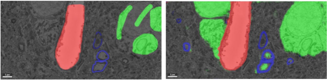
Manual annotations (left) and convolutional network inference (right) of a subset of the labeled voxel classes: blood vessel (red), myelin (blue), and cell body (green). False positive identifications of cell body voxels are visible in the automated inference (inside the myelinated area).
Flood-filling Networks (Architecture, Training, Inference)
Architecture
The FFN comprised a stack of 3d convolutions in SAME mode (input and output of every layer of equal size, with input implicitly padded with zeros to achieve this) with skip connections, rectified linear (ReLU) nonlinearities 24, 3x3x3 kernel sizes, and 32 feature maps in every layer but the the last layer. The network consisted of 19 convolutional layers containing a total of 472,353 trainable weights (see Fig. 5). The input module consisted of a sequence of a 3d convolution, ReLU nonlinearity, and another 3d convolution. This was followed by eight residual modules that performed a ReLU nonlinearity, 3d convolution, ReLU nonlinearity, and 3d convolution. The last layer performed a voxel-wise convolution that combined input from all feature maps (1×1×1 kernel size with a single output feature map). The input and output of the network were equal in spatial size -- 33×33×17 voxels. The input was formed by a 2-channel image, containing EM data in channel 1 (normalized to 0 mean and unit standard deviation) and the current state of the predicted object mask in logit form in channel 2. The output of the network was the updated state of the predicted object mask in logit form.

Architecture of the FFN. The internal modular architecture used here corresponds to “full pre-activation residual modules” 39. The architecture was chosen because in our experiments it showed better convergence than alternatives (no skip connections, or other proposed variants of skip connections 40). We note that our network contains significantly fewer weights than those used in many recent works (e.g. 74x times fewer than 18).
The FFN was implemented in TensorFlow 35 and trained with voxelwise cross-entropy loss:
 where pi is the predicted voxel value and gi is the ground truth label after smoothing. Training proceeded for 7 days using asynchronous stochastic gradient descent at a learning rate of 0.001, in a distributed setting with 32 NVIDIA Tesla K40 GPUs and batches of 4 examples.
Training example sampling
The initial set of training examples was formed by extracting all subvolumes 49 × 49 × 25 voxel in size and fully contained within one of the 33 regions densely segmented by human annotators. The size of the subvolume was chosen to allow FoV movement by one 8-voxel step in every direction.
The ground truth segmentation within every subvolume was binarized by setting voxels belonging to the same object as that of the central voxel of the subvolume to 0.95, and the rest of the voxels to 0.05. These soft labels 24 provided the desired object mask probability map that the FFN was trained to predict.
For every one of the initial training examples, the fraction (fa) of active mask voxels was a calculated. The training examples were then partitioned into 17 classes, such that an example was assigned to class i if ti−1 ≤ fa < ti, and t= (0.0, 0.01, 0.02, 0.03, 0.04, 0.05, 0.06, 0.075, 0.1, 0.2, 0.3, 0.4, 0.5, 0.6, 0.7, 0.8, 0.9, 1). For example, a training example with fa = 0.5 would be a assigned to class 12. During training, each of the 17 classes was sampled equally often.
Seed selection
The seed points for FFN inference were selected as follows: all pixels where the 3d Sobel-filtered EM image was larger than the same image filtered with a Gaussian with σ = 49/6 was set to 1, and 0 otherwise. We then computed the Euclidean distance transform of the resulting binary image and selected local peaks of that transform as the initial FFN seeds.
These seeds were then consumed serially in raster order. All seeds found to be within 3 voxels or less from an existing segment at the time of the inference start were discarded.
Field of View movement procedure
The FoV of the FFN was moved using the following procedure. A list (Q) of positions to be visited was initialized with a location obtained from the seed policy. In the segmentation loop, a location (x, y, z) was extracted from the head of Q, and the FoV was moved to that position, which was then marked as visited. Visited locations were stored in order to ensure that every location was visited at most once during segmentation of an object; locations were stored at 8x reduced resolution in the XY directions and 4x reduced resolution in the Z direction. This reduced resolution effectively determines the minimum step size by which the FoV can be moved, and was used to control the efficiency of inference.
After an inference call, all POM voxels within the FoV were updated, except those that were previously updated by the FFN, had a prior value < 0.5, and a new value larger than the prior value (this biased the network towards splits in areas where predictions of background/foreground were not consistent between iterations). A cuboid of POM values (x-Δx <= x <= x + Δx) ⸀ (y-Δy <= y <= y + Δy) ⸀ (z-Δz <= z <= z + Δz) was then extracted, and the maximum value was then identified on every one of its faces. Whenever this value matched or exceeded the movement threshold of 0.9, the corresponding location was appended to Q unless it was visited before.
The inference loop was terminated when Q was empty. At that point, if the number of voxels with POM values >= 0.6 was >= 1000, a new segment was created consisting of those voxels, otherwise the POM values were reset to 0.05 without creating a segment. Segmentation was terminated when no more seeds were available to start new inference runs. We used Δx = Δy = 8, Δz = 4 which were the largest values that did not result in an increased number of errors in our tests, while remaining computationally tractable.
Criterion for model evaluation and selection
In addition to the densely labeled ground truth data, a 560x560x250-voxel region of the J0126 volume was exhaustively skeletonized by human annotators using Knossos, resulting in 221 skeleton fragments within the subvolume. We used this subvolume to optimize the FFN performance.
During training, a snapshot of the network weights (“checkpoint“) was saved every hour. After training was completed, we ran FFN inference over the densely skeletonized subvolume with every available checkpoint, and evaluated the resulting segmentation with skeleton metrics. We selected the checkpoint that had the highest expected run length among the set of checkpoints with the least number of mergers (in our case this corresponded to the set of checkpoints with zero mergers).
Distributed inference
In order to perform FFN inference efficiently over the whole 663 GB dataset, we split it into overlapping 500x500x500-voxel subvolumes. The subvolume corners were located on a regular grid with a step size of 436 pixels, so that neighboring subvolumes overlapped by 64 voxels in every direction. We ran FFN inference as described above for every subvolume independently, distributing the computational load over a cluster of machines that contained GPUs.
The global segmentation was built using these partial segmentations. A “core” segmentation was extracted from every subvolume by discarding a 32-voxel wide envelope (a subset of the overlap area) and computing connected components of the remaining segmentation. For every face of a subvolume A, a 1-voxel thick plane parallel to this face was extracted from the middle of the overlap area. A corresponding plane was extracted from the neighboring subvolume B sharing the given face. For every segment sA in the A plane, the maximally overlapping (by number of shared voxels) segment sB-A was identified, and vice-versa. Segments for which sA-B = sB-A, i.e. which were mutually maximally overlapping, were then merged. This conservative merging procedure was used in order to avoid spurious mergers (−84%) when creating the global segmentation, at a cost of increased splits (+28%).
Multiresolution oversegmentation consensus
The oversegmentation-consensus procedure relies on intersecting objects in voxel-space. In the case of consensus between segmentations at different resolutions, we upsampled the lower resolution segmentation with nearest neighbors interpolation. We then applied seeded watershed segmentation to the Euclidean distance transform of the higher resolution segmentation as the height map using the upsampled segmentation as seeds. This did not change the topology of the upsampled segmentation, but prevented voxel-level differences between the two segmentations from generating new segments in the oversegmentation-consensus procedure.
To reduce the number of splits in the multi-resolution oversegmentation-consensus procedure, the lower resolution segmentation was filtered by eliminating all objects containing fewer than 100,000 voxels before upsampling. Any object consisting of fewer than 1000 voxels was also removed after consensus.
Cell body segmentation
We created a separate segmentation containing only cell bodies, and used it as a starting point for all subsequent FFN inference. To do so, we performed three FFN inference runs at resolutions of 9x9x20 nm (original), 18x18x20 nm and 36x36x40 nm, with areas of the volume not classified as a cell body by the tissue type classifier masked out. We then applied multi-resolution oversegmentation-consensus, and removed all objects with fewer than 10M voxels. The segmentation was resampled at an isotropic resolution of 160 nm. At this resolution, we computed the Euclidean distance transform within the cell body segments, and used seeded watershed with manually placed seeds (cell body center annotations) to separate adjacent cell bodies. The corrected segmentation was upsampled back to the original resolution of the dataset, and the separated cell bodies were used as seeds for a watershed transform. Background voxels of the full-resolution uncorrected cell body segmentation were masked out so that no new voxels were labeled by watershed.
Flood-Filling Network Agglomeration
Candidate object pair generation
A subset of all possible supervoxel pairs were considered for automated agglomeration. Specifically, we computed agglomeration scores (see below for details) for any pair of objects where both supervoxels contained at least one voxel within the same 5x5x5 cuboid radius. For each such supervoxel pair, we also computed a “decision point” defined as the midpoint of the shortest line that connects any two points of the supervoxels.
For every such decision point involving two objects, A and B, both containing at least 10,000 voxels, we extracted a (101×101×51)-voxel subvolume of EM data and segmentation, centered at the decision point. We then removed the segments A and B from the subvolume, and ran FFN inference within it twice -- once starting from a voxel originally labeled as A, and once starting from a voxel originally labeled as B. To identify the starting voxel, we computed the Euclidean distance transform of the segment A or B, and chose the voxel with maximum distance as the FFN seed point. In case the inference run failed to generate an object covering at least 60% of the voxels of the original object (A or B), a cuboid area of radius (8, 8, 4) voxels around the seed point was zeroed-out in the distance transform, and FFN inference was attempted again from a new location selected as described above. This procedure was repeated up to 16 times.
Agglomeration scoring
We analyzed the FFN inference results for every candidate object pair as follows. The POMs were thresholded at 0.5 to generate a binary segmentation. We computed the number of voxels in the generated segments (NA, NB -- starting from the original segment A, and B, respectively), the fraction of voxels of the original segments within the analysis subvolume reconstructed in the generated segment (fAA, fAB, fBA, fBB),, the Jaccard index JAB between the two segments (defined as the size of the intersection of the two sets of object mask voxels divided by the size of the union of the two sets of object mask voxels), and the number of “deleted” voxels dA, dB, where a voxel in the POM was considered “deleted” if during inference it was updated by the FFN from a value >= 0.8 to a value <= 0.5.
Agglomeration steps
We performed three runs of FFN agglomeration. The first run covered all decision points. The second run was limited to decision points affected by tissue irregularities. Specifically, we computed the cross-correlation of neighboring (z + 1) and next-neighboring (z + 2) sections within the agglomeration subvolume and computed local shift vectors as described in “Tissue irregularity detection”, yielding mz and mz+1. If mz satisfied the tissue irregularity criteria, but mz+2 did not, then we assumed that a single-slice imaging artifact had been identified and replaced section z + 1 with image data from section z + 2. The subvolume was then realigned with translation-only alignment utilizing the neighboring slice shift vectors, and FFN inference was performed without shift masking. The third run was performed with a subvolume of larger size -- (201×201×101) voxels, and was limited to decision points that in the first run resulted in fA* or fB* < 0.4.
We then merged segments A and B if fAA, fAB, fBA, fBB >= 0.6 (at least 60% of the voxels of both original segments were reconstructed in both runs), dA/NA < 0.02 or dB/NB < 0.02 (only a small fraction of the object mask voxels got “deleted” during inference, in at least one of the runs), and JAB >= 0.8 (segmentations starting from A and B were mutually consistent in voxel space). We then treated the merged segments as a weighted graph, with the segments as nodes and JAB as edge weights, computed the connected components of this graph, and checked if any of the components contained more than one segment associated with a cell body (a cell body-cell body merger). If it did, we identified the shortest path between two such cell body segments, and removed the edge with the lowest weight along that path. This procedure was repeated until all mergers were resolved. All parameters used above were optimized using the “validation” set of 12 ground truth skeletons.
Acknowledgements
We thank Tom Dean and Blaise Agüera y Arcas for useful discussions and support. We also thank Michale Fee and Jon Shlens for comments on the manuscript.


