

Abstract
We developed a biologically detailed multiscale model of mouse primary motor cortex (M1) microcircuits, incorporating data from several recent experimental studies. The model simulates at scale a cylindrical volume with a diameter of 300 µm and cortical depth 1350 µm of M1. It includes over 10,000 cells distributed across cortical layers based on measured cell densities, with close to 30 million synaptic connections. Neuron models were optimized to reproduce electrophysiological properties of major classes of M1 neurons. Layer 5 corticospinal and corticostriatal neuron morphologies with 700+ compartments reproduced cell 3D reconstructions, and their ionic channel distributions were optimized within experimental constraints to reproduce in vitro recordings. The network was driven by the main long-range inputs to M1: posterior nucleus (PO) and ventrolateral (VL) thalamus PO, primary and secondary somatosensory cortices (S1, S2), contralateral M1, secondary motor cortex (M2), and orbital cortex (OC). The network local and long-range connections depended on pre- and post-synaptic cell class and cortical depth. Data was based on optogenetic circuit mapping studies which determined that connection strengths vary within layer as a function of the neuron’s cortical depth. The synaptic input distribution across cell dendritic trees – likely to subserve important neural coding functions – was also mapped using optogenetic methods and incorporated into the model. We employed the model to study the effect on M1 of increased activity from each of the long-range inputs, and of different levels of H-current in pyramidal tract-projecting (PT) corticospinal neurons. Microcircuit dynamics and information flow were quantified using firing rates, oscillations, and information transfer measures (Spectral Granger causality). We evaluated the response to short pulses and long time-varying activity arising from the different long-range inputs. We also studied the interaction between two simultaneous long-range inputs. Simulation results support the hypothesis that M1 operates along a continuum of modes characterized by the degree of activation of intratelencephalic (IT), corticothalamic (CT) and PT neurons. The particular subset of M1 neurons targeted by different long-range inputs and the level of H-current in PT neurons regulated the different modes. Downregulation of H-current facilitated synaptic integration of inputs and increased PT output activity. Therefore, VL, cM1 and M2 inputs with downregulated H-current promoted an PT-predominant mode; whereas PO, S1 and S2 inputs with upregulated H-current favored an IT-predominant mode, but a mixed mode where upper layer IT cells in turn activated PT cells if H-current was downregulated. This evidenced two different pathways that can generate corticospinal output: motor-related inputs bypassing upper M1 layers and directly projecting to PT cells, and sensory-related inputs projecting to superficial IT neurons in turn exciting PT cells. These findings provide a hypothetical mechanism to translate action planning into action execution. Overall, our model serves as an extensible framework to combine experimental data at multiple scales and perform in silico experiments that help us understand M1 microcircuit dynamics, information flow and biophysical mechanisms, and potentially develop treatments for motor disorders.
1 Introduction
Primary motor cortex (M1) microcircuits exhibit many differences with those of other cortices – e.g., visual [59] – and with the traditional “canonical” microcircuit proposed by Douglas and Martin almost 30 years ago [12]. These include differences in the cytoarchitecture, cell classes and long and local connectivity. Notable characteristics that demarcate mouse M1 from sensory cortices are a narrower layer 4 and wider layer 5B [70], and its strongly assymetrical projection: upper layer intratelencephalic (IT) cells connect to layer 5B pyramidal-tract (PT) cells but PT cells do not project back [68, 2]. Corticocortical and corticostriatal cells in superficial layers seem to play a role in recurrently processing information at a local level and within thalamocortical and striatal regions, whereas deep corticospinal cells output information (motor commands) from M1 to spinal cord circuits [52, 68, 2]. These distinctions have profound consequences in terms of understanding neural dynamics and information processing [58], and should therefore be considered when developing detailed biophysical models of M1.
We developed a detailed model of M1 microcircuits that combines data at multiple scales from multiple studies: including cell classes morphology, physiology, densities and proportions; and long-range, local, and dendritic-level connectivity. Most data was obtained from studies on the same species and region – mouse M1 – and combined into a single theoretical framework. To integrate all these experimental findings we developed several methodological novelties including specifying connections as a function of normalized cortical depth (NCD) instead of the standard layers, and incorporating projection-specific dendritic distributions of synaptic inputs extracted from subcellular Channelrhodopsin-2-Assisted Circuit Mapping (sCRACM) studies [21, 63]. Additionally, we developed a novel tool, NetPyNE, to help develop, simulate and analyze data-driven biological network models in NEURON [55] (www.netpyne.org).
Our model, which contains over 10 thousand neurons, 30 miliion synapses and models a cylindric cortical volume with a depth of 1350 µm and a diameter of 300 µm constitutes the most biophysically detailed model of mouse M1 microcircuits available. It enables studying the non-intuitive dynamics and interactions occurring across multiple scales, with a level of resolution and precision which is not yet available experimentally. Cortical circuits can have extremely disparate responses to changes in their cellular and subcellular properties; detailed simulation provides a means to systematically explore the circuit-level consequences of manipulations of the cellular components and wiring of the system.
In this study we explore the effect on M1 of increased activity from the different long-range inputs projecting into M1; and of regulation of H-current in PT corticospinal cells. We evaluate the hypothesis that different that M1 operates along a continuum of modes characterized by the level of activation of intratelencephalic (IT), corticothalamic (CT) and PT neurons, and that long-range inputs and H-current modulates which of these modes predominate. To do this, we first demonstrate our model exhibits spontaneous neural activity and oscillations consistent with M1 microcircuits. We then study its response to short pulses and long time-varying signals as inputs to S2 and M2, both independently and simultaneously, and with two different levels of PT H-current.
2 Methods
2.1 Morphology and physiology of neuron classes
Seven excitatory pyramidal cell and two interneuron cell models were employed in the network. Their morphology and physiological responses are summarized in Fig. 1.

A) Volume, cell density per layer, populations, number of cells, and morphologies; B) Proportion of cell classes per layer; C) f-I curve for each excitatory and inhibitory cell class. All properties were derived from published experimental data. Populations labels include the cell class and layer, e.g. ‘IT2’ represents the IT class neurons in layer 2/3.
In previous work we developed layer 5B PT corticospinal cell and L5 IT corticostriatal cell models that reproduce in vitro electrophysiological responses to somatic current injections, including sub- and super-threshold voltage trajectories and f-I curves [46, 62]. To achieve this we optimized the parameters of the Hodgkin-Huxley neuron model ionic channels – Na, Kdr, Ka, Kd, HCN, CaL, CaN, KCa – within a range of values constrained by literature. The corticospinal and corticostriatal cell model morphologies had 706 and 325 compartments, respectively, digitally reconstructed from 3D microscopy images. Morphologies are available via NeuroMorpho.org [?] (archive name “Suter Shepherd”). We further improved the PT model by 1) increasing the concentration of Ca2+ channels (“hot zones”) between the nexus and apical tuft, following parameters published in [19]; 2) lowering dendritic Na+ channel density in order to increase the threshold required to elicit dendritic spikes, which then required adapting the axon sodium conductance and axial resistance to maintain a similar f-I curve; 3) replacing the HCN channel model and distribution with a more recent implementation by Migliore [43]. The new HCN channel reproduced a wider range of experimental observations than our previous implementation [29], including the change from excitatory to inhibitory effect in response to synaptic inputs of increasing strength [16]. This was achieved by including a shunting current proportional to Ih. We tuned the HCN parameters (lk and  ) – originally developed for a CA3 pyramidal neuron [43] – and passive parameters to reproduce these experimental findings using the corticospinal cell, while keeping its somatic f-I curve consistent with recordings [62].
The network model includes five other excitatory cell classes: layer 2/3, layer 4, layer 5B and layer 6 IT neurons and layer 6 CT neurons. Since our focus was on the role of L5 neurons, other cell classes were implemented using simpler models as a trade-off to enable running a larger number of exploratory network simulations. Previously we had optimized 6-compartment neuron models to reproduce somatic current clamp recordings from two IT cells in layers 5A and 5B. The layer 5A cell had a lower f-I slope (X) and higher rheobase (X) than that in layer 5B (X and X). Based on our own and published data, we found two broad IT categories based on projection and intrinsic properties: corticocortical IT cells found in upper layers 2/3 and 4 which exhibited a lower f-I slope (avg X) and higher rheobase (avg X) than IT corticostriatal cells in deeper layers 5A, 5B and 6 (avg X and X) [70, 62, 49]. CT neurons’ f-I rheobase and slope (X and X) was closer to that of corticocortical neurons [49]. We therefore employed the layer 5A IT model for layers 2/3 and 4 IT neurons and layer 6 CT neurons, and the layer 5B IT model for layers 5A, 5B and 6 IT neurons. We further adapted cell models by modifying their apical dendrite length to match the average cortical depth of the layer, thus introducing small variations in the firing responses of neurons across layers.
We implemented models for two major classes of GABAergic interneurons [18]: parvalbumin-expressing fast-spiking (PV) and somatostatin-expressing low-threshold spiking neurons (SOM). We employed existing simplified 3-compartment (soma, axon, dendrite) models [30] and increased their dendritic length to better match the average f-I slope and rheobase experimental values of cortical basket (PV) and Martinotti (SOM) cells (Neuroelectro online database [64]).
2.2 Microcircuit composition: neuron locations, densities and ratios
We modeled in full scale a cylindric volume of mouse M1 cortical microcircuits with a 300 µm diameter and 1350 µm height (cortical depth) with a total of 10,171 neurons Fig. 1A. The cylinder diameter was chosen to approximately match the horizontal dendritic span of a corticospinal neuron located at the center, consistent with the approach used in the HBP model of rat S1 microcircuits [40]. Mouse cortical depth and boundaries for layers 2/3, 4, 5A, 5B and 6 were based on our published experimental data [68, 2, 70]. Although traditionally M1 has been considered an agranular area lacking layer 4, we recently identified M1 pyramidal neurons with the expected prototypical physiological, morphological and wiring properties of layer 4 neurons [70], and therefore incorporated this layer in the model.
Cell classes present in each layer were determined based on mouse M1 studies [18, 62, 2, 70, 49, 30, 45]. IT cell populations were present in all layers, whereas the PT cell population was confined to layer 5B, and the CT cell population only occupied layer 6. SOM and PV interneuron populations were distributed in each layer, with layer 4 and 5B sharing the same populations. Neuronal densities (neurons per mm3) for each layer Fig. 1A were taken from a histological and imaging study of mouse agranaular cortex [65]. The proportion of excitatory to inhibitory neurons per layer was obtained from mouse S1 data [34]. The proportion of IT to PT and IT to CT cells in layers 5B and 6, respectively, were both estimated as 1:1 [18, 62, 71]. The ratio of PV to SOM neurons per layer was estimated as 2:1 based on mouse M1 and S1 studies [27, 67] (Fig. 1B). Since data for M1 layer 4 wasn’t available, interneuron populations labeled PV5A and SOM5A occupy both layers 4 and 5A. The number of cells for each population was calculated based on the modeled cylinder dimensions, layer boundaries and neuronal proportions and densities per layer.
2.3 Local connectivity
We calculated local connectivity between M1 neurons Fig. 2A by combining data from multiple studies. Data on excitatory inputs to excitatory neurons (IT, PT and CT) was primarily derived from mapping studies using whole-cell recording, glutamate uncaging-based laser-scanning photostimulation (LSPS) and channelrhodopsin-2-assisted circuit mapping (CRACM) analysis [68, 2, 70, 71]. Connectivity data was postsynaptic cell class-specific and employed normalized cortical depth (NCD) instead of layers as the primary reference system. Unlike layer definitions which are interpreted differently, NCD provides a well-defined, consistent and continuous reference system, depending only on two readily-identifiable landmarks: pia (NCD=0) and white matter (NCD=1). Incorporating NCD-based connectivity into our model allowed us to capture wiring patterns down to a 100 µm spatial resolution, well beyond traditional layer-based cortical models. M1 connectivity varied systematically within layers. For example, the strength of inputs from layer 2/3 to L5B corticospinal cells depends significantly on cell soma depth, with upper neurons receiving much stronger input [2].
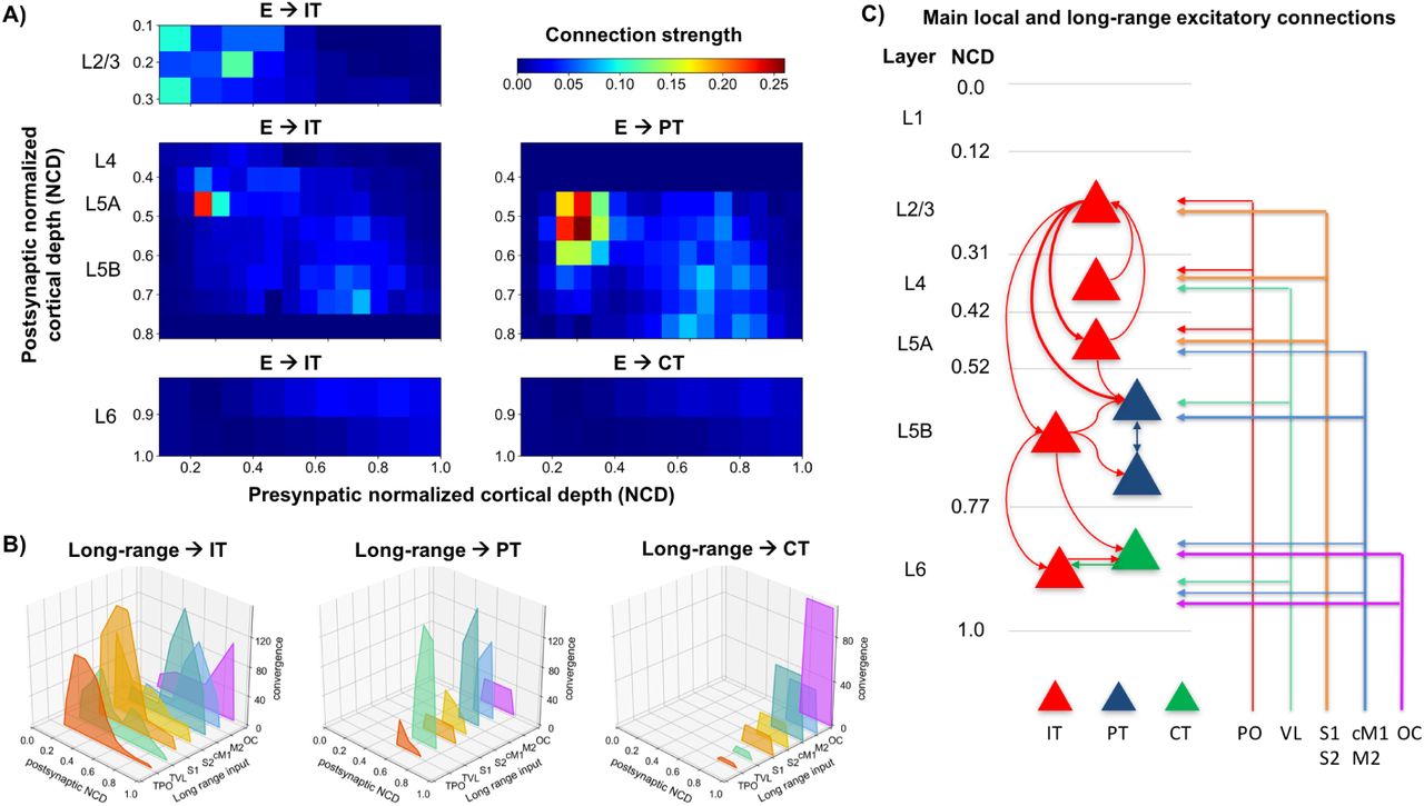
A) Strength of local excitatory connections as a function of pre- and post-synaptic normalized cortical depth (NCD) and post-synaptic cell class; B) Convergence of long-range excitatory inputs from seven thalamic and cortical regions as a function post-synaptic NCD and cell class; C) Schematic of main local and long-range excitatory connections (thin line: medium; thick line: strong).
Connection strength thus depended on presynaptic NCD and postsynatic NCD and cell class. For postsynaptic IT neurons with NCD ranging from 0.0 to 0.3125 (layer 2/3) and 0.8125 to 1.0 (layer 6) we determined connection strengths based on data from [68] with cortical depth resolution of 140 µm-resolution. For postsynaptic IT and PT neurons with NCD between 0.3125 and 0.8125 (layers 4, 5A and 5B) we employed connectivity strength data from [2] with cortical depth resolution of 100 µm. For postsynaptic CT neurons in layer 6 we used the same connection strengths as for layer 6 IT cells [68], but reduced to 62% of original values, following published data on the circuitry of M1 CT neurons [71].
Diagonal elements in the connectivity matrices were increased by 20% to compensate for the underestimates resulting from LSPS CRACM analysis. Our data [71] also suggested that connection strength from layer 4 to layer 2/3 IT cells was similar to that measured in S1, so for these projections we employed values from Lefort’s S1 connectivity strength matrix [34]. Experimentally, these connections were found to be four times stronger than in the opposite direction – from layer 2/3 to layer 4 – so we decreased the latter in the model to match this ratio.
Following previous publications [28, 34], we defined connection strength (scon) between two populations, as the product of their probability of connection (pcon) and the unitary connection somatic EPSP amplitude in mV (icon), i.e. scon = pcon × icon. We employed this equivalence to disentangle the connection scon values provided by the above LSPS studies into pcon and icon values that we could use to implement the model. First, we rescaled the LSPS raw current values in pA [2, 68, 70, 71] to match scon data from a paired recording study of mouse M1 L5 excitatory circuits [28]. Next, we calculated the M1 NCD-based icon matrix by interpolating a layerwise unitary connection EPSP amplitude matrix of mouse S1 [34], and thresholding values between 0.3 and 1.0 mV. Finally, we calculated the probability of connection matrix as pcon = scon/icon.
To implement icon values in the model we calculated the required NEURON connection weight of an excitatory synaptic input to generate a somatic EPSP of 0.5 mV at each neuron segment. This allowed us to calculate a scaling factor for each segment that converted icon values into NEURON weights, such that the somatic EPSP response to a unitary connection input was independent of synaptic location. This is consistent with experimental evidence showing synpatic conductances increased with distance from soma, to normalize somatic EPSP amplitude of inputs within 300 µm of soma [38]. Following this study, scaling factor values above 4.0 – such as those calculated for PT cell apical tufts – were thresholded to avoid overexcitability in the network context where each cell receives hundreds of inputs that interact nonlinearly [60, 4]. For morphologically detailed cells (layer 5A IT and layer 5B PT), the number of synaptic contacts per unitary connection (or simply, synapses per connection) was set to five, an estimated average consistent with the limited mouse M1 data [22] and rat S1 studies [6, 40]. Individual synaptic weights were calculated by dividing the unitary connection weight (icon) by the number of synapses per connection. Although the method does not account for nonlinear summation effects [60], it provides a reasonable approximation and enables employing a more realistic number and spatial distribution of synapses, which may be key for dendritic computations [36]. For the remaining cell models, all with six compartments or less, a single synapse per connection was used.
For excitatory inputs to inhibtory cell types (PV and SOM) we started with the same values as for IT cell types but adapted these based on the specific connectivity patterns reported for mouse M1 interneurons [3, 71] Fig. 2A. Following the layer-based description in these studies, we employed three major subdivisions: layer 2/3 (NCD 0.12 to 0.31), layers 4, 5A and 5B (NCD 0.31 to 0.77) and layer 6 (NCD 0.77 to 1.0). We increased the probability of layer 2/3 excitatory connections to layers 4, 5A and 5B SOM cells by 50% and decreased that to PV cells by 50% [3]. We implemented the opposite pattern for excitatory connections arising from layer 4,5A,5B IT cells such that PV interneurons received stronger intralaminar inputs than SOM cells [3]. The model also accounts for layer 6 CT neurons generating relatively more inhibition than IT neurons [71]. Inhibitory connections from interneurons (PV and SOM) to other cell types were limited to neurons in the same layer [27], with layers 4, 5A and 5B combined into a single layer [45]. Probability of connection decayed exponentially with the distance between the pre- and post-synaptic cell bodies with length constant of 100 µm [15, 14].
Excitatory synapses consisted of colocalized AMPA (rise, decay τ : 0.05, 5.3 ms) and NMDA (rise, decay τ : 15, 150 ms) receptors, both with reversal potential of 0 mV. The ratio of NMDA to AMPA receptors was 1.0 [44], meaning their weights were each set to 50% of the connection weight. NMDA conductance was scaled by 1/(1 + 0.28 · Mg · exp (−0.062 · V)); Mg = 1mM [26]. Inhibitory synapses from SOM to excitatory neurons consisted of a slow GABAA receptor (rise, decay τ : 2, 100 ms) and GABAB receptor, in a 90% to 10% proportion; synapses from SOM to inhibitory neurons only included the slow GABAA receptor; and synapses from PV to other neurons consisted of a fast GABAA receptor (rise, decay τ : 0.07, 18.2). The reversal potential was −80 mV for GABAA and −95 mV for GABAB. The GABAB synapse was modeled using second messenger connectivity to a G protein-coupled inwardly-rectifying potassium channel (GIRK) [11]. The remaining synapses were modeled with a double-exponential mechanism.
Connection delays were estimated as 2 ms plus a variable delay depending on the distance between the pre- and postsynaptic cell bodies assuming a propagation speed of 0.5 m/s.
2.4 Long-range input connectivity
We added long-range input connections from seven regions that are known to project to M1: thalamus posterior nucleus (TPO), ventro-lateral thalamus (TVL), primary somatosensory cortex (S1), secondary somatosensory cortex (S2), contralateral primary motor cortex (cM1), secondary motor cortex (M2) and orbital cortex (OC). Each region consisted of a population of 1000 [9, 6] spike-generators (NEURON VecStims) that generated independent random Poisson spike trains with uniform distributed rates between 0 and 2 Hz [69, 20]; or 0 to 20 Hz [23, 25] when simulating increased input from a region. Previous studies provided a measure of normalized input strength from these regions as a function of postsynaptic cell type and layer or NCD. Broadly, TPO [70, 71, 45], S1 [39] and S2 [63] projected strongly to IT cells in layers 2/3, 4 and 5A; TVL projected strongly to PT cells and moderately to IT cells [70, 71, 45]; cM1 and M2 projected strongly to IT and PT cells in layers 5B and 6 [21]; and OC projected strongly to layer 6 CT and IT cells [21]. We implemented these relations by estimating the maximum number of synaptic inputs from each region and multiplying that value by the normalized input strength for each postsynaptic cell type and NCD range. This resulted in a convergence value – average number of synaptic inputs to each postsynaptic cell – for each projection Fig. 2B. We fixed all connection weights (unitary connection somatic EPSP amplitude) to 0.5 mV, consistent with rat and mouse S1 data [22, 9].
To estimate the maximum number of synaptic inputs per region, we made a number of assumptions based on the limited data available Fig. 2B. First, we estimated the average number of synaptic contacts per cell as 8234 by rescaling rat S1 data [42] based on our own observations for PT cells [62] and contrasting with related studies [56, 10]; we assumed the same value for all cell types so we could use convergence to approximate long-range input strength. We assumed 80 % of synaptic inputs were excitatory vs. 20 % inhibitory [10, 40]; out of the excitatory inputs, 80 % were long-range vs. 20 % local [40, 61]; and out of the inhibitory inputs, 30 % were long-range vs. 70 % local [61]. Finally, we estimated the percentage of long-range synaptic inputs arriving from each region based on mouse brain mesoscale connectivity data [48] and other studies [41, 6, 42, 72, 5]: TVL, S1, cM1 each contributed 15 %, whereas TPO, S2, M2 and OC each accounted for 10 %.
2.5 Dendritic distribution of synaptic inputs
Experimental evidence demonstrates the location of synapses along dendritic trees follows very specific patterns of organization that depend on the brain region, cell type and cortical depth [51, 63]; these are likely to result in important functional effects [32, 33, 60]. We employed subcellular Channelrhodopsin-2-Assisted Circuit Mapping (sCRACM) data to estimate the synaptic density along the dendritic arbor – 1D radial axis – for inputs from TPO, TVL, M2 and OC to layers 2/3, 5A, 5B and 6 IT and CT cell [21] (Fig. 3A), and from layer 2/3 IT, TVL, S1, S2, cM1 and M2 to PT neurons [63] (Fig. 3B). To approximate radial synaptic density we divided the sCRACM map amplitudes by the dendritic length at each grid location, and averaged across rows. Once all network connections had been generated, synaptic locations were automatically calculated for each cell based on its morphology and the pre- and postsynaptic cell type-specific radial synaptic density function (Fig. 3C). Synaptic inputs from PV to excitatory cells were located perisomatically (50 µm around soma); SOM inputs targeted apical dendrites of excitatory neurons [45, 27]; and all inputs to PV and SOM cells targeted apical dendrites. For projections where no data synaptic distribution data was available – IT/CT, S1, S2 and cM1 to IT/CT cells – we assumed a uniform dendritic length distribution.

Synaptic density profile (1D) along the dendritic arbor for inputs from A) TPO, TVL, M2 and OC to layers 2/3, 5A, 5B and 6 IT and CT cells; and B) layer 2/3 IT, TVL, S1, S2, cM1 and M2 to PT neurons. C) Synaptic locations automatically calculated for each cell based on its morphology and the pre- and postsynaptic cell type-specific radial synaptic density function. Here TVL-¿PT and S2-¿PT are compared and exhibit partially complementary distributions.
2.6 Model implementation, simulation and analysis
The model was developed using parallel NEURON [37] and NetPyNE [55] (www.neurosimlab.org/netpyne), a Python package to facilitate the development of biological neuronal networks in the NEURON simulator. NetPyNE emphasizes the incorporation of multiscale anatomical and physiological data at varying levels of detail. It converts a set of simple, standardized high-level specifications in a declarative format into a NEURON model. NetPyNE also facilitates organizing and running parallel simulations by taking care of distributing the workload and gathering data across computing nodes. It also provides a powerful set of analysis methods so the user can plot spike raster plots, LFP power spectra, information transfer measures, connectivity matrices, or intrinsic time-varying variables (eg. voltage) of any subset of cells. To facilitate data sharing, the package saves and loads the specifications, network, and simulation results using common file formats (Pickle, Matlab, JSON or HDF5), and can convert to and from NeuroML, a standard data format for exchanging models in computational neuroscience. Simulations were run on XSEDE supercomputers Comet and Stampede using the Neuroscience Gateway (NSG) and our own resource allocation.
3 Results
3.1 Activity patterns in M1 network
We characterized expected in vivo spontaneous activity that would be driven by long-range inputs from the 7 characterized input regions firing at a baseline level distributed uniformly for each input stream in range of 0 to 2 Hz (Fig. 4). Overall firing rates ranged up to 20 Hz for excitatory populations, with 40 Hz for inhibitory populations, consistent with the in vivo recordings from multiple cortical areas in rat and mouse [23, 35, 50, 13]. Additionally, the distribution of cell average firing rates was highly skewed and long tailed, providing a lognormal distribution (Fig. 4B).

A) Top: 1 sec raster plot. Cells are grouped by population and ordered by NCD within each population. Note that no lines are given for the locations of the particular layers since those boundaries are always somewhat indeterminate (a motivation for using NCD). Bottom: Example IT5A and PT5B voltage traces. B) Distribution of average firing rates for the different classes of excitatory (( top)) and inhibitory (( bottom)) (across 4 seconds). C) Scatter plot (blue dots) and binned mean and standard deviation (green line) of PT5B firing rates as a function of cell normalized cortical depth (NCD) (across 4 seconds).
Activity patterns were not only dependent on cell class and cortical-layer location, but also sublaminar location, demonstrating the importance of identifying connectivity and organizing simulations by NCD rather than layer [18, 2]. PT cell activity within layer 5B was particularly high at the top of L5b and decreased with cortical depth (Fig. 4C), consistent with the strong sublaminar targeting of local projections and of long-range connections [2, 68].
3.2 Field activity and information flow
Simulated LFP recordings from the M1 model revealed physiological oscillations in the beta and gamma range (Fig. 5). These emerged in the absence of rhythmic external inputs, and are therefore a consequence of neuronal biophysical properties and circuit connectivity. To our knowledge, this is the first data-driven, biophysically-detailed model of M1 microcircuits that exhibits spontaneous physiological oscillations without rhythmic synaptic inputs. Beta-band oscillations peaked at 28 Hz and were robust across the full 4-second simulation; gamma oscillations were weaker and its peak varied across time between 40 and 80 Hz (Fig. 5B,C). Strong LFP beta and gamma oscillations are characteristic of motor cortex activity in both rodents [8, 66] and monkeys [54, 47]. Spectral Granger Causality analysis revealed strong information flow from IT2 cells to IT5A and PT5B, and from IT5A to PT5B, but not from PT5B to upper layer IT cells (Fig. 5D). These results confirm information flow follows known microcircuit functional connectivity depicting M1 as a system with a preprocessing-like upper-layer loop that unidirectionally drives lower-layer output circuits [68]. Information flow frequency peaks coincided with LFP beta and gamma bands, both of which play a predominant role in information coding during preparation and execution of movements [1, 66].

A) LFP signal averaged across 11 recording electrodes at different depths (200 µm to 1300 µm at 1300 µm interval). B) Power spectral density (PSD) with peaks at beta and gamma frequencies, characteristic of cortical activity. Physiological oscillations emerged in the absence of rhythmic external inputs. C) LFP spectrogram with a consistently strong beta frequency peak and weaker gamma frequency peaks across 4 seconds. D) Spectral Granger causality shows strong information flow at beta frequency from IT2 to IT5A and PT5B, and from IT5A to PT5B, but not in the opposite direction.
3.3 Sensory-related pathways and H-current modulation
Modulation of H-current level in conjunction with sensory-related long-range inputs lead to different modes of operation in M1. Increased rates (average 15 Hz for 100 ms) in PO, S1 or S2 together with an upregulated H-current favored an IT-predominant mode (with low PT activity) – Fig. 6 (high Ih) shows results for the S2 input case. The same long-range input levels with H-current downregulated lead to a mixed mode where upper layer IT cells in turn activated PT cells (Fig. 6, low Ihcase). Analysis across 25 simulations with different wiring and input randomization seeds demonstrated a statistically significant increase in PT5B average and peak firing rates for low vs. highIh Downregulation of H-current facilitated synaptic integration of inputs and increased PT output activity. This constitutes one of the pathways that can generate corticospinal output: sensory-related inputs projecting to superficial IT neurons in turn exciting PT cells.

A) Raster plots of M1 in response to increased S2 activity (15 Hz for 100 ms) after 400 ms, with high (left) vs low (right) PT5B Ih. B) Temporal spike histogram of S2, IT2, IT5A and PT5B populations for high vs low PT Ihlevel; inset figures shows PT5B peak rate before and after S2 pulse. High Ihresults in IT-predominant mode, whereas low Ihresults in a mixed mode with both IT and PT activity. C) Schematic of main pathways activated due to S2 increased activity. D) Boxplot analysis showing statistically significant higher average and peak PT5B firing rate in response to S2 input for low vs. high PT5B Ihlevel. Analysis performed across 25 simulations with 5 different connectivity randomization seeds × 5 different spiking input randomization seeds.
3.4 Motor-related pathways and H-current modulation
Motor-related inputs bypassing upper M1 layers and directly projecting to PT cells constitute a second pathway that can result in corticospinal output. Increased activation (average 15 Hz for 100 ms) of VL, cM1 and M2 inputs with downregulated H-current promoted a PT-predominant mode with lower IT activity – Fig. 7 (lowIh) shows results for the M2 input case. As with sensory-related inputs, upregulation of H-current in corticospinal cells also decreased their activity (Fig. 7 highIh)). Analysis across 25 simulations with different wiring and input randomization seeds demonstrated a statistically significant increase in PT5B average and peak firing rates for low vs. high Ih. This effect was stronger than for sensory-related inputs.

A) Raster plots of M1 in response to increased M2 activity (15 Hz for 100 ms) after 400 ms, with high (left) vs low (right) PT5B Ih. B) Temporal spike histogram of M2, IT2, IT5A and PT5B populations for high vs low PT Ihlevel; inset figures shows PT5B peak rate before and after M2 pulse. Low Ihlevel results in PT-predominant mode. C) Schematic of main pathways activated due to M2 increased activity. D) Boxplot analysis showing statistically significant higher average and peak PT5B firing rate in response to M2 input for low vs. high PT5B Ihlevel. Analysis performed across 25 simulations with × 5 different connectivity randomization seeds 5 different spiking input randomization seeds.
3.5 Interaction between sensory- and motor-related pathways and H-current modulation
M1 response to increased activation from S2 and M2 inputs depended strongly on the order of presentation, interval between inputs and PT Ihlevel (Fig. 8).For IT5A cells, lower Ihincreased activity only when the S2 input occurred before M2. IT5A activity exhibited significantly stronger average and peak rates when S2 was presented before M2. In that case, average IT5A rates increased with interval indicating summation of inputs; whereas with M2 inputs first, there was no clear pattern in relation to interval. Peak IT5A rates plateaued after 20 ms interval when S2 was presented first, indicating peak was determined by the S2 input. However, when M2 was presented first, IT5A rates showed the inverse pattern, decreasing proportional to interval, suggesting dominance of the M2 input.

A) Raster plot of M1 in response to increased S2 and M2 activity (15 Hz for 100 ms) with S2 starting at 400 ms and M2 100 ms (interval) later; PT5B was low. B) Average (left) and peak (right) post-stimulus IT5A (top) and PT5B (bottom) firing rate for different intervals (x-axis), order of presentation (blue: M2-S2; red: S2-M2), and high (dotted) vs low (solid) Ihlevels. C) Schematic of main pathways activated due to S2 and M2 increased activity. Varying interval between presentation of inputs illustrated with δt symbol.
Lower Ihconsistently resulted in higher activity in PT5B neurons, independently of order and interval (Fig. 8). PT5B average rate increased with interval if S2 came before M2, but decreased with interval if M2 input was first. This suggests initial S2 input results in PT5B having a longer integration window which enables summation of the M2 inputs. Peak PT5B rates were constant when S2 input arrived first – suggesting S2 dictated its peak rate – but presented a strong peak at 60 ms interval when M2 arrived first. This might indicate resonance at the beta frequency range, consistent with our previous observation (Fig. 4).
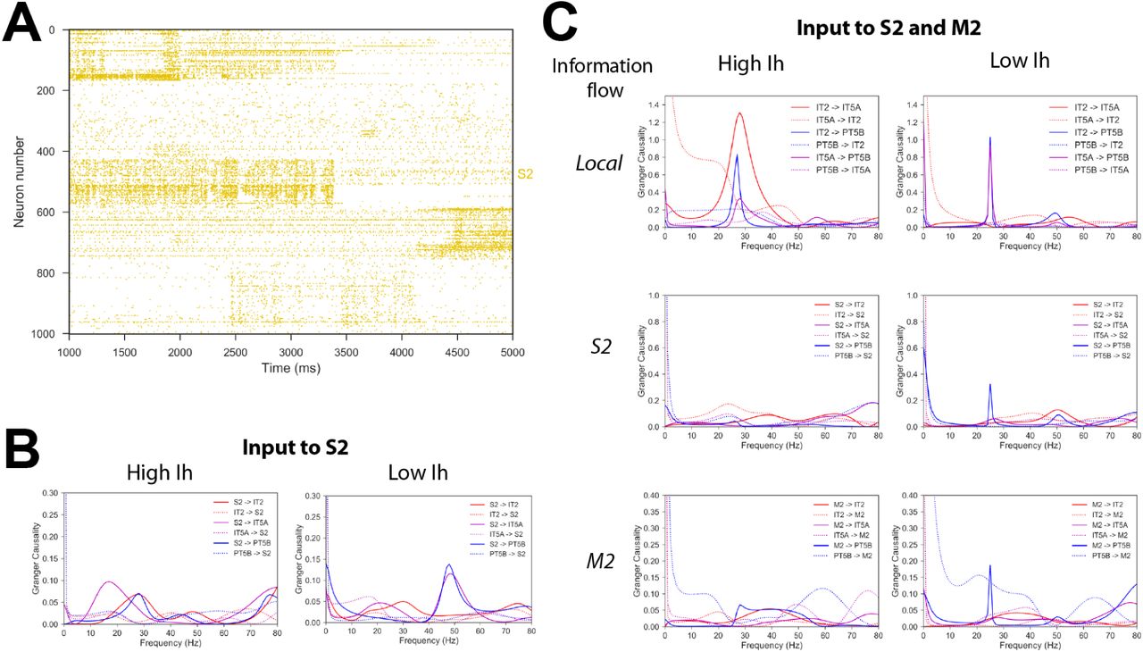
3.6 Information flow in response to recorded time-varying spiking activity
Time-varying spiking activity recorded from mouse somatosensory cortex – 4 second duration, average rate of 2.77 Hz – was used as S2 input (Fig. 9A). With high Ih, information flow, quantified using Spectral Granger causality, was strongest from S2 to IT5A and was concentrated in the beta frequency range. With low Ih, information flow shifted to the gamma frequency range and was strongest from S2 to PT5B (Fig. 9B). This provides further support for the role of Ihin modulating the flow of information to corticospinal output and switching between the IT-predominant mode and a mixed mode with both IT and PT activity.
A) Raster plot of time-varying spiking activity recorded from mouse somatosensory cortex. B) Spectral Granger causality when using the recorded spiking data (A) as input to S2; shows increase of information flow from S2 to PT5B in the gamma frequency range for low vs. high Ih. C) Spectral Granger causality between populations when using the recorded spiking data (A) as input to M2 and a different recorded pattern as input to S2; shows increase in information flow from upper layer ITs (IT2 and IT5A) to PT5B and from long-range inputs (S2 and M2) to PT5B in the beta frequency range for low vs. high Ih.
A different set of recordings – also 4 second duration, average rate of 3.84 Hz – was simultaneously used as input to M2, to evaluate the interactions between S2 and M2 inputs. With high Ih, information flow was strongest among upper layers (IT2 to IT5A), but was very low from S2 and M2 to any of the local populations. This suggests simultaneous activation resulted in destructive interference of the signal. Lowering Ihresulted in increased information flow peaks at beta frequency from IT2, S2 and M2 to PT5B, again suggesting Ihas a potential mechanism to enable information to reach corticospinal neurons (Fig. 9C).
Recordings of neuron spiking activity in mouse somatosensory cortex were downloaded from CRCNS.org [24]. The recordings were performed in vitro with a large and dense multielectrode array. The data represents spontaneous activity given that the culture was not stimulated. Spike trains were filtered to include only those with an average firing rate between 0.1 and 50 Hz.
4 Discussion
In this study we developed the most detailed computational model of mouse M1 microcircuits and corticospinal neurons up to date, based on an accumulated set of experimental studies. Overall, the model incorporates quantitative experimental data from 15 publications, thus integrating previously isolated knowledge into a unified framework. Unlike the real brain, this in silico system serves as a testbed that can be probed extensively and precisely, and can provide accurate measurements of neural dynamics at multiple scales. We employed the model to evaluate how long-range inputs from surrounding regions and molecular/pharmacological-level effects (e.g. regulation of HCN channel) modulate M1 dynamics.
The M1 simulation reproduced several experimental observations. The reported lognormal distribution of firing rates in our model has been found extensively in cortical networks [53, 31]. The simulation tied a key structural property – different upper vs lower layer 5B wiring – to differentiated circuit-level neural dynamics and function – higher activity in upper layer 5B. The LFP beta and gamma oscillations have been measured in rodent and primate motor cortices and may be fundamental to the relation of brain structure and function [7].
We simulated the inputs from the main cortical and thalamic regions that project to M1, based on recent experimental data from optogenetic mapping studies. Consistent with experimental data [21, 63], this study evidenced two different pathways that can generate corticospinal output: motor-related inputs from VL, cM1 or M2 regions bypassing upper M1 layers and directly projecting to corticospinal cells, and sensory-related inputs from PO, S1 and S2 regions projecting to superficial IT neurons in turn exciting layer 5B corticospinal cells. Activation of OC region lead to increased layer 6 IT and CT activity and physiological oscillations in the beta and gamma range. Downregulation of corticospinal H-current lead to increased firing rate and information flow, as observed experimentally. This has been hypothesized as a potential mechanism to translate action planning into action execution [57]. Our model also provides insights into the interaction between sensory- and motor-related inputs, suggesting that the order and interval between inputs determines its effect on corticostriatal and corticospinal responses.
Our study provides insights to help decipher the neural code underlying the brain circuits responsible for producing movement, and help understand motor disorders, including spinal cord injury. The computational model provides a framework to integrate experimental data and can be progressively extended as new data becomes available. This provides a useful tool for researchers in the field, who can use the framework to evaluate hypothesis and guide the design of new experiments. A recent study on closed-loop optogenetics suggests employing models of cortical microcircuits to guide patterned stimulation that restores healthy neural activity [17].
5 Acknowledgements
This work was funded by the following grants: NIH U01EB017695, NYS SCIRB DOH01-C32250GG-3450000 and NIH R01EB022903.
References
- [1].↵
- [2].↵
- [3].↵
- [4].↵
- [5].↵
- [6].↵
- [7].↵
- [8].↵
- [9].↵
- [10].↵
- [11].↵
- [12].↵
- [13].↵
- [14].↵
- [15].↵
- [16].↵
- [17].↵
- [18].↵
- [19].↵
- [20].↵
- [21].↵
- [22].↵
- [23].↵
- [24].↵
- [25].↵
- [26].↵
- [27].↵
- [28].↵
- [29].↵
- [30].↵
- [31].↵
- [32].↵
- [33].↵
- [34].↵
- [35].↵
- [36].↵
- [37].↵
- [38].↵
- [39].↵
- [40].↵
- [41].↵
- [42].↵
- [43].↵
- [44].↵
- [45].↵
- [46].↵
- [47].↵
- [48].↵
- [49].↵
- [50].↵
- [51].↵
- [52].↵
- [53].↵
- [54].↵
- [55].↵
- [56].↵
- [57].↵
- [58].↵
- [59].↵
- [60].↵
- [61].↵
- [62].↵
- [63].↵
- [64].↵
- [65].↵
- [66].↵
- [67].↵
- [68].↵
- [69].↵
- [70].↵
- [71].↵
- [72].↵


