

ABSTRACT
The primary challenge of fixed-backbone protein sequence design is to find a distribution of sequences that fold to the backbone of interest. In practice, state-of-the-art protocols often find viable but highly convergent solutions. In this study, we propose a novel method for fixed-backbone protein sequence design using a learned deep neural network potential. We train a convolutional neural network (CNN) to predict a distribution over amino acids at each residue position conditioned on the local structural environment around the residues. Our method for sequence design involves iteratively sampling from this conditional distribution. We demonstrate that this approach is able to produce feasible, novel designs with quality on par with the state-of-the-art, while achieving greater design diversity. In terms of generalizability, our method produces plausible and variable designs for a de novo TIM-barrel structure, showcasing its practical utility in design applications for which there are no known native structures.
1 Introduction
Computational protein design has emerged as powerful tool for studying the conformational space of proteins, and has allowed us to expand the space of known protein folds [1, 2, 3, 4, 5, 6], create variations on existing topologies [7, 8, 9, 10, 11], and access the expansive space of sequences yet to be traversed by evolution [12]. These advances have led to significant achievements in the engineering of therapeutics [13, 14, 15], biosensors [16, 17, 18], enzymes [19, 20, 21, 22], and more [23, 24, 25, 26, 27]. Key to such successes are robust sequence design methods that allow for the selection of amino acid sequences that minimize the folded-state energy of a pre-specified backbone conformation, which can be either derived from native structures or designed de novo. This difficult task is often described as the “inverse” of protein folding—given a protein backbone, design an amino acid sequence such that the designed sequence folds into that conformation.
The existence of many structural homologs with low sequence identity suggests that there should be many foldable sequences for a given protein backbone [28, 29]. In other words, for naturally occurring protein backbones at least, there should be not a unique sequence, but rather a distribution of sequences that fold into the target structure. This range of diverse homologs arise through evolution, where mutations that largely preserve the structure and/or function of proteins can propagate, and impactful experimental methods that mimic evolution have been able to recapitulate this sequence diversity in vitro [30, 31]. Computational design methods that capture this variability would allow for the discovery of sequences that fold to the desired topology, while encoding a range of structural properties and possibly new and varying functions. Current approaches that operate on fixed backbone templates fall short in this regard.
Common approaches for fixed-backbone sequence design involve specifying an energy function and sampling sequence space to find a minimum-energy configuration. Methods for optimizing over residues and rotamers include variations on the dead-end elimination (DEE) algorithm [32, 33, 34, 35], integer linear programming [36, 37], belief propagation [38, 39], and Markov Chain Monte Carlo (MCMC) with simulated annealing [40, 41, 42]. One of the most successful sequence design methods, and the only one to have been broadly experimentally validated, is RosettaDesign, which solves the sequence design problem by performing Monte Carlo optimization of the Rosetta energy function [43] over the space of amino acid identities and rotamers [44, 45]. A significant limitation of fixed-backbone sequence design methods is that designs tend to have little sequence diversity; that is, for a given backbone, design algorithms tend to produce highly similar sequences [41, 46].
Well-tolerated amino acid mutations are often accompanied by subtle backbone movements, due to resulting rearrangement of side-chains. For fixed-backbone design, the template backbone is intended to serve as a reference for the final desired structure, but traditional design methods which optimize atomic-level energy functions are often highly constrained by the initial backbone, and as a result they tend to converge to a limited range of solutions. Ideally, even with a fixed protein backbone as the input, a design algorithm should infer sequences that fold back to the input structure in a manner that preserves the original topology with minor deviations, while allowing exploration of a vast array of diverse solutions. This would be practical for general sequence exploration, e.g. for library design for directed evolution [47], and could be particularly useful in the case of de novo design, where starting backbones have no known corresponding sequence and might have errors that limit the accuracy of energy-function-based design.
In practice, generating diverse designs with Rosetta often requires either manually manipulating amino acid identities at key positions [7, 9], adjusting the energy function [48, 49], or explicitly modeling perturbations of the protein backbone [50, 51, 52, 53]. However, it is often the case that incorporation of residues not justified by established principles and not energetically favorable under current molecular mechanics frameworks can in fact be crucial. Design methods that account for flexibility of the protein backbone often use “softer” potentials [49, 54], including statistical potentials derived from data [55, 56, 55, 57, 58]. These types of methods, however, often have worse performance compared to well-parameterized molecular mechanics force fields.
With the emergence of deep learning systems, which can learn patterns from high-dimensional data, it is now possible to build models that learn complex functions of protein sequence and structure, for example models for protein backbone generation [59] and protein structure prediction [60]. We hypothesized that a deep learning approach would also be effective in developing a new, fully learned statistical potential that could be used for design.
In this study, we establish a novel method for fixed-backbone sequence design using a learned deep convolutional neural network (CNN) potential. This potential predicts a distribution over amino acid identities at a residue position conditioned on the environment around the residue in consideration. For a candidate protein backbone, we iteratively sample from the conditional distributions encoded by the neural network at each residue position in order to design sequences. Our goal in developing this method was to assess the degree to which a softer potential could learn the patterns necessary to design highly variable sequences, without sacrificing the quality of the designs.
Without any human-specified priors and simply by learning directly from crystal structure data, our method produces realistic and novel designs with quality on par with Rosetta designs under several key metrics, while achieving greater sequence diversity. We computationally validate designed sequences via ab initio forward folding. We also test the generalization of our method to a de novo TIM-barrel scaffold, in order to showcase its practical utility in design applications for which there are no known native structures.
1.1 Related Work
The network we train is a 3D convolutional neural network (CNN). CNNs [61] are a powerful class of models that have achieved state-of-the-art results across machine learning tasks on image, video, audio input, in addition to other modalities [62, 63, 64, 65]. The model we train is similar to that presented in [66], but we note that any trained model to predict amino acid identity given the residue’s local environment, including those that use spherical convolutions [67, 68], could be used to guide sampling as well. Previous machine learning models for this particular task have only been applied to architecture class, secondary structure, and ΔΔG prediction [66, 67, 68].
Most relevant to this work are statistical potentials which explicitly model local sequence and structure features at residue positions to perform sequence design [55, 57, 58, 69, 70, 71]. These approaches involve writing down statistical energy functions [72], where terms are a function of the probability of sequence or structural features and correspond to unary, pairwise, or higher-order interactions between these elements. In this paper, we seek to learn a statistical potential to guide design that can take into account higher-order residue and backbone interactions by construction and that does not require fitting a fixed statistical model to data.
Similar to our approach in motivation is recent work on graph-based protein sequence generation [73], where an autoregressive transformer (self-attention) model [74] is used over a graph representation of the input backbone atoms to sample a range of sequences that should fold into the starting structure. This method models the joint distribution of sequence residues given backbone atoms, while we model local conditional probabilities given a candidate sequence. Our hypothesis is that, unlike in language models for example where certain words or phrases can greatly affect the likelihood of a distal word [75, 76, 77, 78], for protein structures the local sequence context constraints residue identity.
Recent work on using machine learning to guide rotamer packing is also similar in inspiration to our method [79], although we tackle the broader problem of sequence discovery. This method involves learning an energy function for rotamer state by training a network with positive examples from data and negative examples drawn from the known distribution of rotamers. While we considered such energy-based models (EBMs) for sequence design, we decided against this type of approach because in practice many amino acid substitutions at particular positions might be viable, making it non-trivial to select negative examples for training.
Other studies that attempt to leverage machine learning for the structure-guided sequence design task include using neural networks to individually predict residues in a sequence [80, 81], building a variational autoencoder conditioned on protein topology to generate designs [82], and framing protein design as a constraint-satisfaction problem and training a graph neural network to find designs [83]. None of the aforementioned methods validate designs either across a range of biochemical metrics of interest or by folding in silico or in vivo, with the exception of [83] who provide preliminary CD (circular dichroism) spectra data. Moreover, these methods do not prove to have comparable or improved performance relative to Rosetta sequence design. In this study, we do an in-depth analysis of the distribution of sequences produced by our method in an effort to establish that our method is immediately useful for design tasks.
2 Methods
An overview of our method is presented in Figure 1. We train a deep convolutional neural network to predict amino acid identity given the residue’s local environment, consisting of all neighboring backbone and side-chain atoms within a fixed field-of-view, masking the side-chain atoms of the residue of interest. The classifier defines a distribution over amino acid types at each sequence position.
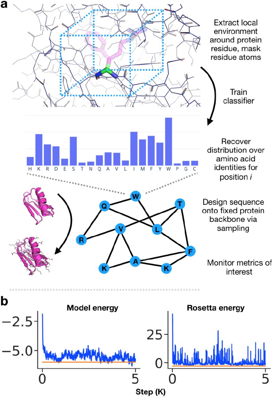
a) We train a deep convolutional neural network to predict amino acid identity given the local environment around the residue (box not to scale). The network provides a distribution over amino acid types at each residue position for the protein. Sequences are designed onto fixed protein backbones via blocked Gibbs sampling. b) Metrics of interest are monitored during sampling (orange – native, blue – samples).
Given a candidate protein backbone for which a corresponding sequence is desired, starting with a random initial sequence, we iteratively sample amino acid identities from the conditional probability distribution defined by the classifier network in order to design sequences.
2.1 Sampling algorithm
Given a backbone structure X for an n residue protein, we are interested in sampling from the true distribution of sequences Y given X,

We assume that the identity of each residue yi is entirely determined by its local context, namely the identities of its neighboring residues yNB(i) and backbone atoms X.
Under this assumption, the input backbone X defines a graph structure, where nodes correspond to residues yi and edges exist between pairs of residues (yi, yj) within some threshold distance of each other. We can think of this graph as a Markov Random Field (MRF), where each residue yi is independent of all residues conditioned on those in its Markov blanket, i.e.

Gibbs sampling
If we had access to the the true conditional distributions p(yi|yNB(i); X) for each residue, by doing Gibbs sampling over the graph, we would be able draw samples as desired from the joint distribution P (Y|X). Gibbs sampling is an MCMC algorithm and involves repeatedly sampling values for each variable conditioned on the assignments of all other variables [84].
We train a network to learn these conditional distributions from data. For a residue yi, given backbone atoms X and neighboring residues yNB(i), our trained classifier outputs pθ(yi|yNB(i); X), a distribution over amino acid types where pθ(yi|yNB(i); X) ≈ p(yi|yNB(i); X). We use the trained network to specify the conditional distributions for a Gibbs sampler over the graph. Although the learned distribution pθ(yi|yNB(i); X) is only an approximation of the true conditional distribution, if the learned conditionals were to match the true data conditionals, then a Gibbs sampler run with the learned conditionals would have the same stationary distribution as a Gibbs sampler run with the true data conditionals [85].
In order to speed up convergence, we do blocked Gibbs sampling of residues. In practice, we draw edges in the graph between nodes where corresponding residues have Cβ atoms that are less than 20 Å apart, guaranteeing that non-neighboring nodes correspond to residues that do not appear in each other’s local environments. During sampling, we use greedy graph coloring to generate blocks of independent residues. We then sample over all residues in a block in parallel, repeating the graph coloring every several iterations.
Model energy
We can approximate the joint probability of a sequence P (Y|X) with the pseudo-log-likelihood (PLL) [86] of the sequence under the model, defined as

Note that training the neural network with cross-entropy loss involves maximizing the log probability of the correct residue class given the residue environment; the PLL is the sum over these log probabilities.
Even after a burn-in period, not every sampled sequence is likely viable. We treat the negative PLL as a heuristic model energy, and use it as a metric for selecting low-energy candidate sequences. We opt not to optimize the PLL directly, as this leads to inflated PLLs that are far greater than those of native sequences. There is degeneracy in the residue prediction task, where in many cases there are multiple residues that justifiably fit a local environment with high probability. However, by explicitly optimizing the PLL via simulated annealing, it is possible to converge to sequence patterns that are outside of the input data distribution and yet have inflated probabilities under the neural network, such that, for example, the network is ~ 99% certain about nearly every residue in the sequence. Sampling regularizes against moving away from the manifold of natural sequences.
Since our model does not yet include predictions for rotamer angles (side-chain torsions), we need a way to select a rotamer after we have sampled a candidate residue at a given position. Furthermore, the choice of rotamer might require re-packing of neighboring residue rotamers in order to resolve clashes. We use PyRosetta4, a Python wrapper around Rosetta [87], to optimize all rotamers within a radius of 5 Å from the current residue. This procedure is called each time the model is used to sample a mutation at a particular position. After residues are sampled and mutated, rotamers are consecutively re-packed around each residue in a block in random order.
Runtime
The runtime for our method for sequence design is determined primarily by three steps: (1) sampling residues, (2) computing the model energy (negative PLL), and (3) rotamer repacking. The time to sample residues and compute the model energy is determined by the speed of the forward pass of the neural network, which is a function of the batch size, the network architecture, and the GPU itself. Rotamer repacking time for our method currently scales linearly with the block size.
Baselines
We assess the performance of our sequence design method by comparison with two baselines, which we refer to as Rosetta-FixBB and Rosetta-RelaxBB. The Rosetta-FixBB baseline uses the Rosetta packer [44], invoked via the RosettaRemodel [88] application, to perform sequence design on fixed backbones. This design protocol performs Monte Carlo optimization of the Rosetta energy function over the space of amino acid types and rotamers [44]. Between each design round, side-chains are repacked, while backbone torsions are kept fixed. Importantly, the Rosetta design protocol samples uniformly over residue identities and rotamers, while our method instead samples from a learned conditional distribution over residue identities. The Rosetta-RelaxBB protocol is highly similar to the Rosetta-FixBB protocol but performs energy minimization of the template backbone in addition to repacking between design cycles, allowing the template backbone to move.
The Rosetta-FixBB protocol provides the most relevant comparison to our method as both operate on fixed backbones. However, Rosetta-RelaxBB is the more commonly used mode of sequence design, and generates solutions that are more variable than those of Rosetta-FixBB. We have therefore included designs from both methods for comparison. Starting templates for both baselines have all residues mutated to alanine, which helps eliminate early rejection of sampled residues due to clashes.
2.2 Data
To train our classifier, we used X-ray crystal structure data from the Protein Data Bank (PDB) [89]. We separated structures into train, test, and validation sets based on CATH 4.2 topology classes, splitting classes into roughly 85%, 10%, and 5%, respectively (1161, 140, and 68 classes) [28, 29]. This ensured that sequence and structural redundancy between the datasets was largely eliminated. We used these CATH topology class splits to assign PDB files to train, test, or validation sets. We first applied a resolution cutoff of 3.0 Å, eliminated NMR structures from the dataset, and enforced an S60 sequence identity cutoff to eliminate sequence redundancy. Then, since CATH assignments are done at a protein domain level, we specified that no chain for any PDB in the test set could have a domain belonging to any of the train or validation set CATH topology classes and that no chain for any PDB in the validation set could have a domain belonging to any of the train set CATH topology classes. The resulting total number of PDBs for the train, test, and validation datasets were 21147, 3319, and 964, respectively. When a biological assembly was listed for a structure, we trained on the first provided assembly; otherwise we trained on the original listed crystal structure. This was so that we trained primarily on what are believed to be functional forms of the protein macromolecules, including in many cases hydrophobic protein-protein interfaces that would otherwise appear solvent-exposed.
The input data to our classifier is a 20 × 20 × 20 Å3 box centered on the target residue, and the environment around the residue is discretized into voxels of volume 1 Å3. We keep all backbone atoms, including the Cα atom of the target residue, and eliminate the Cβ atom of the target residue along with all of its other side-chain atoms. We center the box at an approximate Cβ position rather than the true Cβ position, based on the average offset between the Cα and Cβ positions across the training data. For ease of data loading, we only render the closest 400 atoms to the center of the box.
We omit all hydrogen atoms and water molecules, as well as an array of small molecules and ions that are common in crystal structures and/or possible artifacts (Supplementary data). We train on nitrogen (N), carbon (C), oxygen (O), sulfur (S), and phosphorus (P) atoms only. Ligands are included, except those that contain atoms other than N, C, O, S, and P. Bound DNA and RNA are also included. Rarer selenomethionine residues are encoded as methionine residues.
We canonicalize each input residue environment in order to maximize invariance to rotation and translation of the atomic coordinates. For each target residue, we align the N-terminal backbone N − Cα bond to the x-axis. We then rotate the structure so that the normal of the N − Cα − C plane points in the direction of the positive z-axis. Finally, we center the structure at the effective Cβ position. By using this strategy, we not only orient the side-chain atoms relative to the backbone in a consistent manner (in the positive z-direction), but also fix the rotation about the z-axis. We then discretize each input environment and one-hot encode the input by atom type.
2.3 Model training
Our model is a fully convolutional network, with six 3D convolution layers each followed by batch normalization and LeakyReLU activation with a slope of 0.2 [90]. We regularize with dropout layers with dropout probability of 10% and with L2 regularization with weight 5 × 10⁻⁶. We train our model using the PyTorch framework, with default weight initialization [91]. We train with a batch size of 513 parallelized synchronously across three NVIDIA 1080 Ti GPUs. The momentum of our BatchNorm exponential moving average calculation is set to 0.99.
We train the model using the Adam optimizer (β1 = 0.5, β2 = 0.999) with learning rate 1 × 10⁻⁴ [92]. The model starts to overfit around 4 epochs of training, which takes around 24 hours. Our final classifier is an ensemble of four models corresponding to four concurrent checkpoints around the timepoint of peak validation accuracy. Predictions are made by averaging the logits (unnormalized outputs) from each of the four networks.
3 Results
3.1 Trained classifier recapitulates expected biochemical features
We report the performance of our residue classifier in Figure 2. Our ensembled classifier achieves a 57.2% test set accuracy. Compared to other machine learning models for the same task, our model gives an improvement of 14.7% over [66] (42.5%), and similar performance to [67] (56.4%) and [68] (58.0%). We note that we do not use the same train/test sets as these studies. Figures 2a,b show that the predictions of the network correspond well with biochemically justified substitutability of the amino acids. For example, the model often confuses large hydrophobic residues phenylalanine (F), tyrosine (Y), and tryptophan (W), and within this group, more often confuses F and Y which are similarly sized compared to the bulkier W. We believe this type of learned degeneracy is necessary in order for the classifier to be useful for guiding sequence design.
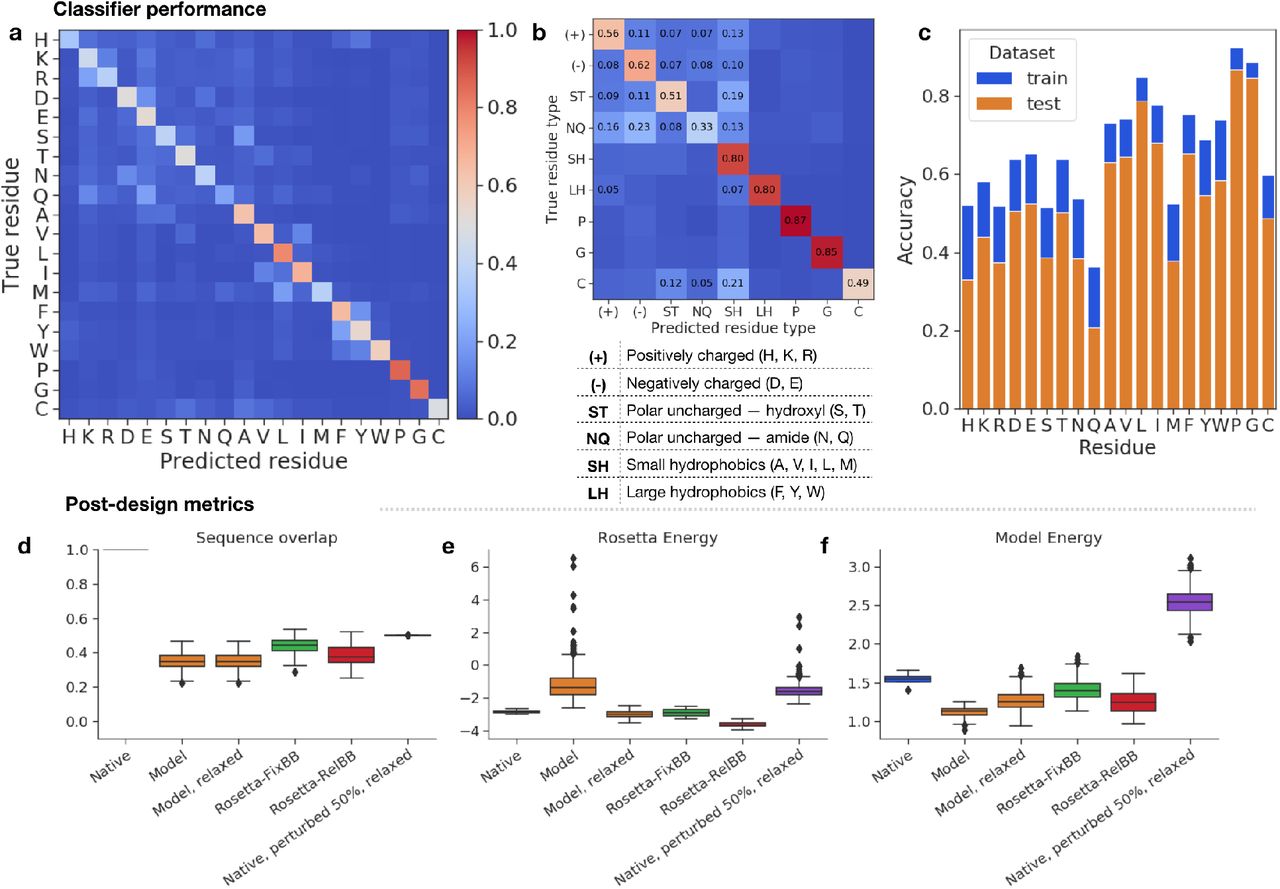
Classifier error/confusion matrices for test set data, at the level of (a) individual residues and (b) groups of biochemically similar residues. Grouping is done to separate charged, polar, and hydrophobic residues. Diagonal entries correspond to class accuracies; off-diagonal entries are errors. Percent error listed for errors ≥ 5%. c) Per-class accuracy for the train and test set. d-f) Sequence design metrics for top 100 sequences across design methods for each of four test cases. Results presented for the native sequence and sequences designed using either our model or one of two Rosetta protocols. d) Percent sequence overlap with native. e) Length-normalized Rosetta energy. f) Length-normalized model energy (negative PLL).
We report class-specific train and test accuracies in Figure 2c. On the whole, the model is more certain about hydrophobic/non-polar residue prediction compared to hydrophilic/polar; this corresponds with the intuition that exposed regions in many cases allow a variety of polar residues, while buried core regions might be more constrained and therefore accommodate a limited set of hydrophobic residues. The model does especially well at predicting glycine and proline residues, both of which are associated with distinct backbone torsion distributions.
3.2 Sampling gives native-overlapping, low-energy candidate sequences
We selected four native structures from the test set as test cases for evaluating our method: PDB entries 1acf, 1bkr, 1cc8 and 3mx7. These structures belong to the beta-lactamase (CATH:3.30.450), T-fimbrin (CATH:1.10.418), alpha-beta plait (CATH:3.30.70), and lipocalin (CATH:2.40.128) topology classes, respectively. We selected these test structures because (1) they span the three major CATH [28, 29] protein structure classes (mostly alpha, alpha-beta, and mostly beta), and (2) their native sequences were recoverable via forward folding with Rosetta AbInitio, ensuring they could serve as a positive control for later in silico folding experiments.
In order to remove potentially confounding artifacts that emerge during construction and optimization of PDB structures, we idealize and relax all inputs under the Rosetta energy function before design. This step is also necessary in order for the Rosetta protocols to in theory be able to recover the native sequence via optimization of the Rosetta energy function.
For each test case, we ran 15 independent sampling trajectories for 5000 iterations each, starting from a random initial sequence with rotamers repacked. The sampling procedure appears to generate good candidate sequences within hundreds of iterations. Sequences from concurrent timepoints of the same trajectory are correlated. Therefore, instead of blindly picking the top model energy sequences across all sampling timepoints, we first found local minima of the model energy over the course of sampling, specifying that the local minima must be below a 5% percentile cutoff of model energy and at least 50 steps apart. From this set of local minima, we selected the top 100 sequences (lowest model energy) across all trajectories for further analysis.
Sampling for 5000 steps takes between 4.5 to 6 hours for the test cases on a Tesla P100 GPU (Supplementary data). Each trajectory gives on average 20 sequences based on our local minima cutoff criteria. This corresponds to about 20-30 minutes per sequence design, which is on par with Rosetta-RelaxBB’s runtime for a single design. Rosetta-FixBB is faster, taking 5-15 minutes per design (Supplementary data).
In Figure 2d, we present post-design summary metrics for the top model-designed sequences and baselines. Over the course of burn-in, the model designs start to near the native sequence. On average, the top model designs recapitulate around 30-40% of the native sequence. The Rosetta-FixBB protocol best recapitulates the native sequence among the design methods; however, since we start with a relaxed backbone for which the native sequence is already a low Rosetta energy solution, it is not unexpected that Rosetta-FixBB should best recover the native sequence.
Although the Rosetta energy is not optimized during our design procedure, many of the designs have relatively low Rosetta energy (Figure 2e), though there is a long tail of high Rosetta energy designs primarily due to side-chain clashing. After relaxing the model designs, their Rosetta energy decreases to match the native backbone, with relatively low subsequent backbone deviation (Figure S2e); in contrast, sequences that are 50% similar to native, with random perturbations, have a high Rosetta energy, even after relax (Figure 2e). The model energy too is similarly low for the model designs and the Rosetta designs, while it is inflated for 50% perturbed native sequences, indicating that the model energy as a heuristic roughly matches Rosetta in differentiating low-energy vs. high-energy designs (Figure 2f).
3.3 Model designs achieve greater sequence diversity than Rosetta designs
One failure mode of Rosetta-FixBB is its convergence to highly similar sequences, a deficiency that is handled somewhat but not entirely by protocols that interleave backbone relaxes during design, such as our baseline Rosetta-RelaxBB protocol and Backrub [51, 52, 53].
To assess the variability of our model-designed sequences relative to Rosetta designs, we first measured the average overlap between sequences relative to the native sequence and across design methods (Figure 3a,b). While the Rosetta designs are highly convergent, the model designs are much more variable.
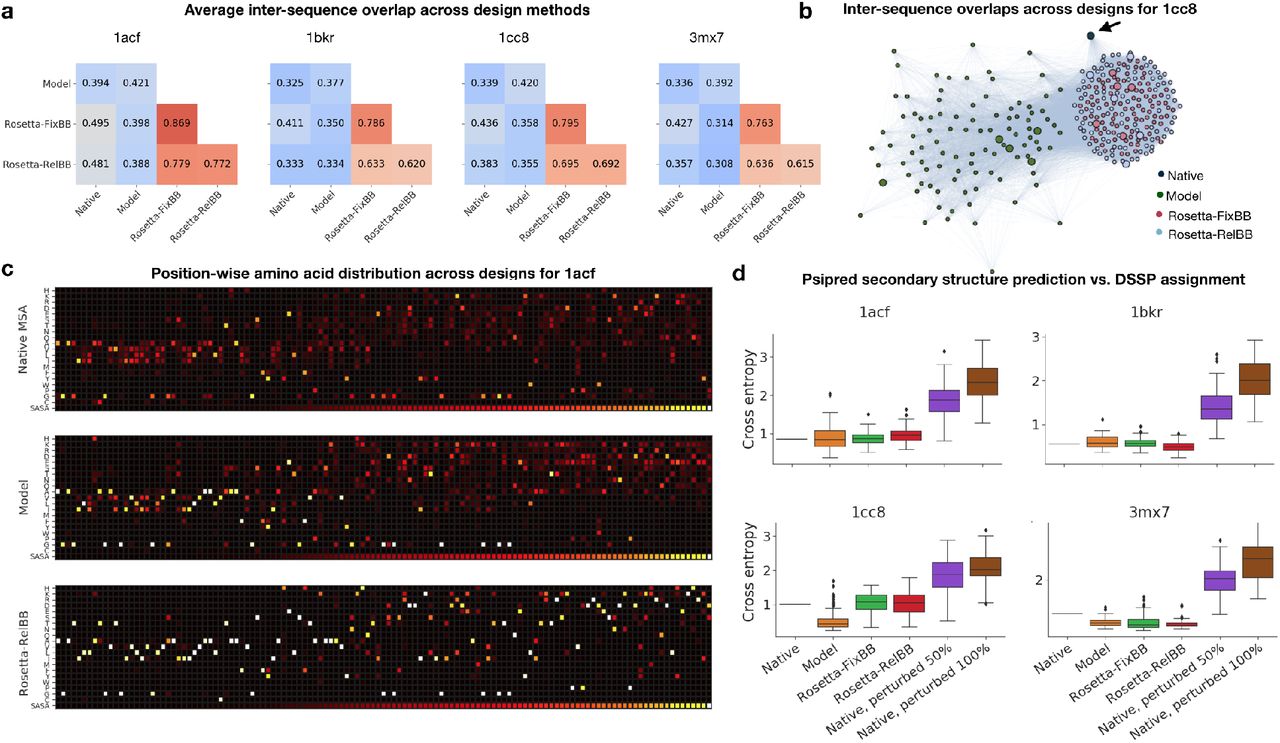
a) Average inter-sequence fractional overlap within and across top sequences from each design method. b) Cluster plot representation of top designs across methods for test case 1cc8. Edges are between sequences with greater than 40% overlap with weights proportional to percent sequence overlap. Larger nodes correspond to top 5 model or Rosetta energy sequences for model designs and Rosetta designs, respectively. Nodes are positioned using the Fruchterman-Reingold force-directed algorithm [101]. c) Position-wise amino acid distributions for test case 1acf. Columns are ordered by increasing solvent-accessible surface area (SASA) of native sequence residues from left to right. (Top) Native sequence and aligned homologous sequences from MSA (n = 424); (Middle) Model designs (n = 100); (Bottom) Rosetta-RelaxBB designs. (n = 100). MSAs obtained using PSI-BLAST v2.9, the NR50 database, BLOSUM62 with an E-value cutoff of 0.1. d) Psipred secondary structure prediction for designed sequences. Cross-entropy of Psipred [94, 95, 96, 97, 98] prediction (helix, loop, sheet) with respect to DSSP assignments [100] for native sequence (n = 1) and designs (n = 100). Psipred predictions are from sequence alone without database alignment.
We then looked into patterns of variability by position, specifically between solvent-exposed and buried regions. In Figure 3c, we show the position-wise amino acid distribution across designs for test case 1acf, sorting the positions by increasing solvent-accessible surface area (SASA) of the native residues [93]. The model designs are more variable in solvent-exposed regions, as are sequences homologous to the native found through MSA; in comparison, the Rosetta protocols are much more convergent. However, both the model designs and Rosetta designs converge to similar core (low SASA) regions (Figure S1a), indicating that perhaps the need for a well-packed core in combination with volume constraints determined by the backbone topology might limit the number of feasible core designs. In general, model designs have higher position-wise entropy (Figures 3c, S1b), while still retaining correct patterns of hydrophobic/non-polar and hydrophilic/polar residue positions at buried and solvent-exposed positions, respectively.

a) Position-wise accuracy vs. solvent accessibility across design methods for four test cases (n = 100, each). Accuracy with respect to native sequence. Solvent-accessible surface area (SASA) calculated for native residues. b) Position-wise entropy vs. solvent accessibility across design methods for four test cases (n = 100, each). Solvent-accessible surface area (SASA) calculated for native residues. c) Psipred secondary structure prediction for designed sequences. Cross-entropy of Psipred [94, 95, 96, 97, 98] prediction (helix, loop, sheet) with respect to DSSP assignments [100]. Psipred predictions from MSA features after UniRef90 [99] database alignment. d) MSA sequence identity overlap for lowest energy designs across design methods. Points represent individual aligned hits (max. 500 hits per sequence). Hits presented for native sequence (n = 1), top 5 model designs under model energy (negative PLL), top 5 Rosetta designs under Rosetta energy for Rosetta-FixBB and Rosetta-RelaxBB. MSAs obtained using PSI-BLAST v2.9, the NR50 database, BLOSUM62 with an E-value cutoff of 0.1. [119, 98, 120].
To confirm that key sequence features are retained despite the increased variability seen, we calculated Psipred [94, 95, 96, 97, 98, 99] secondary structure prediction accuracy relative to DSSP assignments [100] and found that the predictions for model-designed sequences from single sequences alone (Figure 3d) and with MSA features (Figure S1c) are comparable in accuracy to those for the native sequence and Rosetta designs, indicating that despite variation, the designed sequences retain local residue patterns that allow for accurate backbone secondary structure prediction.
Moreover, variability seen among the lowest model energy designs does not arise from the model exactly recapitulating known homologs, as indicated by the low sequence identity between the 5 minimum model energy designs (highlighted in Figure 3b) and their top hits from multiple sequence alignment (MSA) (Figure S1d).
Overall, we find that the model designs are more variable than the Rosetta designs; however, we need to ensure that, despite this variation, the designs have key biochemical features, such as hydrophobic residue packing, formation of polar networks, and helical capping.
3.4 Model designs are comparable to Rosetta designs under a range of biochemically relevant metrics
The ultimate test of any fully redesigned sequence on a fixed backbone is experimental validation that the designed sequence folds back into the intended structure. While it is infeasible to experimentally verify each sequence, we can assess the validity of designed sequences en masse using metrics that are agnostic to any energy function.
Sequences designed onto the test case backbones should ideally have the following key biochemical properties [103, 104]: (1) core regions should be tightly packed with hydrophobic residues, a feature that is important for driving protein folding and maintaining fold stability [105, 106, 107]; (2) designs should have few exposed hydrophobic residues, as these incur an entropic penalty as a result of solvent ordering under the hydrophobic effect and an enthalpic penalty from disrupting hydrogen bonding between polar solvent molecules [108, 109, 93], making it energetically favorable to place polar residues at solvent-accessible positions and apolar residues at buried positions; (3) designed side-chains should form hydrogen bonds to buried donor or acceptor backbone atoms, and if polar residues are designed in core regions, they should be supported by hydrogen bonding networks [110, 23].
To assess these properties of interest we use the following three metrics: (1) packstat, a non-deterministic measure of tight core residue packing [102], (2) exposed hydrophobics, which calculates the solvent-accessible surface area (SASA) of hydrophobic residues [93], and (3) counts of buried unsatisfied backbone (BB) and side-chain (SC) atoms, which are the number of hydrogen bond donor and acceptor atoms on the backbone and side-chains, respectively, that are not supported by a hydrogen bond. We use PyRosetta implementations of these metrics and monitor them over the course of sampling [87].
In Figure 4, we compare our designs to the Rosetta-FixBB and Rosetta-RelaxBB protocol designs, as well as the native idealized structure, across these metrics. Since the designs have less than 50% sequence overlap with the native on average (Figure 2d), we also include data for the native sequence with either 50% or 100% of the residues randomly mutated; these perturbed sequences serve as a negative control and indicate expected performance for likely non-optimal deviations from the native sequence.

Designs (n = 100) compared to native idealized structure (n = 1). 50% and 100% mutated native sequences included as negative controls. a-d) Biochemical metrics of interest. a) Packstat, a measure of core residue packing [102], averaged over 10 measurements. b) Total solvent-accessible surface area (SASA) of exposed hydrophobic residues. [93] c) Number of buried unsatisfied polar backbone (BB) atoms. d) Number of buried unsatisfied polar side-chain (SC) atoms. e) Capping residue placement. Average number of capping residues across top 100 designs for test cases with capping positions. f) Amino acid distribution of designed sequences relative to native sequence and its aligned homologs (max. 500 hits per sequence). MSAs obtained using PSI-BLAST v2.9, the NR50 database, BLOSUM62 with an E-value cutoff of 0.1.
We also report performance across these metrics for designed sequences relaxed with the RosettaRelax protocol (Figure S2). This procedure allows the backbone and rotamers to move to adopt a lower Rosetta energy conformation. Relaxing the designs allows us to assess whether alternate rotamers and deviations of the starting protein backbone can lead to an improvement in performance across the metrics considered.
Packstat. Model designs tend to have a lower packstat score compared to to the native sequence and the Rosetta designs (Figure 4a); however, on average the packstat scores are still higher relative to random perturbations of the native sequence. While this trend seems to indicate that the model designs are less optimal than the Rosetta designs, when we look at the model designs post-relax (Figure S2a), the packstat scores improve and better match those of the native sequence and Rosetta designs, while the perturbed sequence packstat scores remain low. At the same time, the post-relax Cα backbone RMSDs between design methods are also comparable. These results suggest that the designed sequences do tightly pack core regions, as slight movements of the backbone and repacked rotamers for model designs give well-packed structures.
Exposed hydrophobics. Model designs in general do not place exposed hydrophobics in solvent-exposed positions, similar to the native sequence and Rosetta designs (Figure 4b). Random perturbations of the native sequence inevitably place hydrophobic residues in exposed positions, resulting in an inflated exposed hydrophobics score. The native sequence for test case it 3mx7 has many exposed hydrophobic residues, suggesting that the native protein might bind to a target, forming a hydrophobic interface.
Buried unsatisfied backbone atoms. For all of the test cases except 1bkr, model designs have similar or fewer unsatisfied backbone polar atoms compared to the native sequence (Figure 4c). For 1bkr, although the average number of unsatisfied backbone polar atoms is greater than that of the native sequence or Rosetta designs, the distribution is fairly wide, indicating that there are many designs that have fewer unsatisfied backbone polar atoms compared to the native sequence. However, some of the 50% perturbed sequences have fewer unsatisfied backbone polar atoms than the native, suggesting that this metric alone is not sufficient for selecting or rejecting designs.
Buried unsatisfied side-chain atoms. Model designs across test cases have few unsatisfied buried side-chain polar atoms, similar to the native sequences and Rosetta designs (Figure 4d). This indicates that over the course of sampling, side-chains that are placed in buried regions are adequately supported by backbone hydrogen bonds or by design of other side-chains that support the buried residue.

50% and 100% mutated native sequences included as negative controls. As RosettaRelax is non-deterministic, procedure is run 100 times on the native idealized backbone in order to get a distribution of post-relax metrics for the starting scaffold. a-d) Biochemical metrics of interest. a) Packstat, a measure of core residue packing [102], averaged over 10 measurements. b) Total solvent-accessible surface area (SASA) of exposed hydrophobic residues [93]. c) Number of buried unsatisfied polar backbone (BB) atoms. d) Number of buried unsatisfied polar side-chain (SC) atoms. e-f) Post-relax RMSD and energies. e) Alpha carbon RMSD (Å) after relax. f) Rosetta energy post-relax (length-normalized) g) Model energy (negative PLL) post-relax (length-normalized)
Another key structural feature is the placement of N-terminal helix capping residues—typically there will be an aspartic acid (D), asparagine (N), serine (S), or threonine (T) preceding the helix starting residue, as these amino acids can hydrogen bond to the second backbone nitrogen in the helix [111, 112]. The majority of both the model designs and the Rosetta designs successfully place these key residues at the native backbone capping positions (Figure 4e). By inspection, we also see a number of specific notable features across the test cases. These include placement of prolines at cis-peptide positions, placement of glycines at positive ϕ backbone positions, and polar networks supporting loops and anchoring secondary structure elements (Supplementary data).
In Figure 4f, we see that the model designed sequences adhere to an amino acid distribution similar to the native sequence and its aligned homologs, with the most pronounced difference being an apparent overuse of glycine (G), alanine (A), and glutamatic acid (E) relative to the homolog sequences. Rosetta protocols also match this distribution well, with a tendency to overuse small hydrophobic residues, in particular alanine (A) and isoleucine (I). Since the homologous sequences discovered by MSA likely capture amino acid patterns that can anchor and support the given backbones, the similarity of the distributions suggests that the model designs retain viable sequence patterns.
Overall, we see that the model designs are comparable to both the native structures and to the Rosetta-FixBB and Rosetta-RelaxBB protocol designs across a range of metrics (Figures 4, S2).
3.5 Designed sequences are validated by blind structure prediction
We performed blind structure prediction using the AbInitio application in Rosetta [113, 114, 115] to determine whether our designed sequences could adopt structures with low RMS deviation from the starting backbone and low Rosetta energy. AbInitio uses secondary structure probabilities obtained from Psipred (with MSA features after UniRef90 [99] database alignment) to generate a set of candidate backbone fragments at each amino acid position in a protein. These fragments are sampled via the Metropolis-Hastings algorithm to construct realistic candidate structures (decoys) by minimizing Rosetta energy.
For each test case we forward-folded the lowest model energy design in addition to the lowest Rosetta energy designs from Rosetta-FixBB and Rosetta-RelaxBB (Figure 5). All designs were selected without using any external heuristics, manual filtering, or manual reassignments. As an additional benchmark, we included sequences that were randomized to have 50% sequence overlap with the native sequences. We obtained Psipred predictions, “picked” 200 fragments per residue position [115], and ran 104 trajectories per design. For each design, we highlight in red and visualize the best-quality structure as determined by a summed rank of template-RMSD and Rosetta energy (Figure 5).

Native sequences and lowest energy designs were forward folded using Rosetta AbInitio for four design test cases. 50% randomly perturbed native sequences included as a negative control. (Left) Folded structure with best summed rank of template-RMSD and Rosetta energy across 104 folding trajectories. Decoys (yellow) are aligned to the idealized native backbones (blue). Sequence identity and RMSD (Å) compared to native are reported below the structures. For Rosetta-RelaxBB, RMSD of selected design to relaxed structure post-design is given in parentheses. (Right) Rosetta energy vs. RMSD (Å) to native funnel plots. RMSD is calculated with respect to the idealized and relaxed native crystal structure. For Rosetta-RelaxBB, RMSD in funnel plot is with respect to relaxed structure post-design.
We found that, in addition to treating negative PLL as a heuristic model energy, we could use the negative sum of the unnormalized logits of the network as another heuristic to rank sequences. This is given by  where xi are the amino acids of a length n candidate sequence x and E(xi) is the logit for amino acid type xi at position i. This heuristic correlates well with the negative PLL. The scale of the logits tends to correlate with the norm of the inputs, and as a result the logits-based criterion effectively weights core regions more heavily. We found empirically that sequences with low logits-based energy had desirable features. Results for forward-folding top-ranked sequences under the logits-based criterion are given in Figure S3. Note that for test case 1bkr, the top-ranked design under both heuristics is the same.

Sequences forward folded using Rosetta AbInitio for four design test cases. 50% randomly perturbed native sequences included as a negative control. (Left) Folded structure with best summed rank of template-RMSD and Rosetta energy across 104 folding trajectories. Decoys (yellow) are aligned to the idealized native backbones (blue). Sequence identity and RMSD (Å) compared to native are reported below the structures. For Rosetta-RelaxBB, RMSD of selected design to relaxed structure post-design is given in parentheses. (Right) Rosetta energy vs. RMSD (Å) to native funnel plots. RMSD is calculated with respect to the idealized and relaxed native crystal structure. For Rosetta-RelaxBB, RMSD in funnel plot is with respect to relaxed structure post-design.
The model designs had generally low sequence identity to the native sequence (< 43%), but were able to closely recover the native backbones (Figures 5, S3). All of the model designs achieved significantly better recovery than the 50% randomly perturbed cases. Compared to Rosetta-designed structures, our designs tended to have lower sequence identity while achieving comparable or better recovery of the native backbone. These results suggest that (1) close recovery of the native backbone is due to features learned by the model and not simply due to sequence overlap with the native, and (2) that our method is able to generate solutions not accessible via Rosetta design, that differ from native sequences, and yet fold under the Rosetta energy function.
3.6 Application – Model-based sequence design of a de novo TIM-barrel
Design of de novo proteins remains a challenging task as it requires robustness to backbones that lie near, but outside the distribution of known structures. Successful de novo protein designs often lack homology to any known sequences despite the fact that de novo structures can qualitatively resemble known folds [9, 7, 116]. For a design protocol to perform well on de novo backbones it must therefore avoid simple recapitulation of homologous sequences.
To assess whether our model could perform sequence design for de novo structures, we tested our method on a Rosettagenerated four-fold symmetric de novo TIM-barrel backbone, running 25 sampling trajectories for 5000 iterations. The TIM-barrel backbone is a circularly permuted variant of the reported design, 5bvl [7] which was excluded from the training set. While we did not exclude native TIM-barrels from the training set, 5bvl is distant in sequence from any known protein, and contains local structural features that differ significantly from naturally occurring TIM-barrels [7], making it unlikely that the model would return memorized sequences found in the training set as solutions. We note that the original design 5bvl was designed using a combination of Rosetta protocols and manual specification of residues.
We generated sequences for this template using both our model and Rosetta, and found that the model designs were highly variable relative to the Rosetta designs (Figures 6a, S4a,b), rich in biochemical features (Figure S4c), exhibiting dense hydrophobic packing and helical capping, as well as extended hydrogen-bonding networks (Figure 6b). In the core region, which was noted as being highly convergent in the original study [7], designs were variable and yet densely packed (Figure 6c). Model designs also differed noticeably between symmetric units, suggesting that our model is capable of providing a range of solutions for even near-identical backbones (Figure 6d). One possible defect that we observed was the over-use of glycines in negative ϕ positions (Supplementary data).

Native here indicates original design. a) Average inter-sequence fractional overlap within and across top sequences from design methods. b) Position-wise amino acid distributions for TIM-barrel. Columns are ordered by increasing solvent-accessible surface area (SASA) of native sequence residues from left to right. (Top) Model designs; (Bottom) Rosetta-RelaxBB designs (n = 100). c) Sequence design metrics across design methods, pre-RosettaRelax (blue) and post-RosettaRelax (orange). d) Psipred secondary structure prediction for designed sequences. Cross-entropy of Psipred [94, 95, 96, 97, 98] prediction (helix, loop, sheet) with respect to DSSP assignments [100]. (Left) Psipred predictions from MSA features after UniRef90 [99] database alignment. (Right) Psipred predictions from single sequence without database alignment. e) MSA sequence identity overlap for lowest energy designs per design method. Points represent individual aligned hits (max. 500 hits per sequence). Hits presented for native sequence (n = 1), top 5 model designs under model energy (PLL) and logits-based criterion (n = 10), top 5 Rosetta designs under Rosetta energy for Rosetta-FixBB and Rosetta-RelaxBB (n = 5, each). MSAs were obtained using PSI-BLAST v2.9, the NR50 database, BLOSUM62 with an E-value cutoff of 0.1. Sequence alignment for 5bvl was removed. f) Forward folding of baseline designs. Rosetta-FixBB and Rosetta-RelaxBB designs are forward folded using Rosetta AbInitio (Left) Rosetta energy vs. RMSD (Å) to native funnel plots. RMSD is calculated with respect to the idealized and relaxed native crystal structure. For Rosetta-RelaxBB, RMSD of selected design to relaxed structure post-design is given in parentheses. (Right) Reporting folded structure with best summed rank of template-RMSD and Rosetta energy across 104 folding trajectories. Decoy (yellow) aligned to idealized native backbone (blue). Sequence identity overlap with native sequence and RMSD (Å) reported below structure. For Rosetta-RelaxBB, RMSD in funnel plot is with respect to relaxed structure post-design.

a) Variability of designed TIM-barrel sequences. A cluster plot representation of top designs across design methods. The native sequence is shown in blue and indicated with an arrow. Larger nodes correspond to top sequences that are forward folded and shown in (e). Edges are shown between sequences with greater than 40% overlap with weights proportional to percent sequence overlap. Nodes are positioned using the Fruchterman-Reingold force-directed algorithm [101]. b-d) Designed Biochemical Features. The top design (under logits criterion) is shown in (b) with each four-fold symmetric unit shown in a different color. The insert shows an example of a multi-residue polar network designed at the border of two symmetric units. c) Sphere-rendering of the TIM-barrel core. Identical colors between (b) and (c) indicate the same symmetric unit. d) An overlay of the four symmetric units, with the aligned backbone shown in grey, and side chains rendered as sticks. Oxygen atoms are colored red and nitrogen atoms blue. e) Forward folding of designs. Sequences are forward folded using Rosetta AbInitio. (Left) Rosetta energy vs. RMSD (Å) to native funnel plots. RMSD is calculated with respect to the idealized and relaxed native crystal structure. (Right) Reporting folded structure with best summed rank of template-RMSD and Rosetta energy across 104 folding trajectories. Decoy (yellow) aligned to idealized native backbone (blue). Sequence identity overlap with native sequence and RMSD (Å) reported below structure.
Psipred secondary structure predictions from model-designed sequences were fairly accurate (Figure S4d), and a homolog search of the best 3 model energy (negative PLL) and best 3 logits-based energy sequences yielded few hits with low sequence identity, indicating that these designs are novel (Figure S4e)
We performed AbInitio forward-folding of the best three model energy (negative PLL) and best three logits-based energy designs. All of the six selected designs outperformed the 50% randomized sequence baseline in recovering the target backbone, and four of the six designs achieved better or comparable recovery (< +1 Å RMSD) with respect to the original designed sequence (3.5 Å RMSD). Even with low (< 35%) sequence identity to the original design, model designs performed comparably to Rosetta designs that had significantly higher overlap (> 50%) with the native sequence (Figure S4f).
Overall, these results suggest that our method can produce plausible designs with significant variability, even for protein backbones outside the space of known native structures.
4 Discussion
In this paper, we show that sampling with an entirely learned potential encoded by a deep convolutional neural network can give a distribution of possible sequences for a fixed backbone. Our method is able to design sequences which are comparable to those designed by Rosetta protocols across a range of key biochemical metrics, but are far more variable than both. The primary limitation to using a deep neural network to guide sampling is the possibility of artifacts due to the model learning non-robust features from the data [117]. We see indications of this, for example, when our model predicts glycine at some non-standard positions.
There are several possibilities for extending and improving this method. The underlying classifier could be improved by exploring new network architectures, optimization schemes, and input representations. We note that previously reported models for the same task, such as those that use spherical convolutions [67], or improved models that emerge in the future could trivially be swapped in for the classifier network presented without any fundamental change to the method. Similarly, other methods for rotamer repacking could be substituted in as well. Small modifications to the sampling procedure such as introducing ϵ – greedy sampling [118] for exploration noise or resampling lower probability residue positions in a biased manner could give improved designs. We note that the sampling protocol easily allows for adding position-specific constraints during design.
Having the classifier predict side-chain torsions jointly with residue identity would allow us to eliminate the Rosettaguided rotamer repacking step. Then, by parallelizing the sampling procedure across several GPUs, constant scaling as a function of the length of the protein should be feasible, if the batch size per GPU is kept constant. Compressing the network or modifying the architecture could also give speed-ups. These changes should open up avenues for even faster sequence discovery.
We believe that transformer models [74], including graph transformer models like that presented in [73], could be a promising way to model distal sequence patterns. Our results suggest that a convolutional network that looks at a canonicalized local residue environments might be a good way to featurize inputs to such networks and that training via autoencoding conditioned on larger portions of the sequence rather than sequential autoregressive training might be more amenable to modeling protein sequences. Finally, using energy-based models (EBMs) similar to that presented in [79] might also be a promising complementary approach to our method.
Though we evaluated our method against Rosetta in this paper, in practice our method could be combined with Rosetta in a natural way. Rosetta design protocols run MCMC with a uniform proposal distribution over amino acid types and rotamers. One could imagine using the distribution provided by the classifier as a proposal distribution for Rosetta design protocols, potentially speeding up convergence. The model energy, along with other metrics, could also be used to guide early stopping to avoid over-optimization of the Rosetta energy function.
Finally, the ultimate test of any designed sequence is experimental validation in the laboratory. We intend to validate our designed sequences not only by traditional crystal structure determination, but also by high-throughput enzymatic assays as a proxy for folding. Since our approach gives us a range of variable designs, we hope to run high-throughput experiments that allow us to test folding at scale; results from such experiments could help us learn features that predict folding of designed sequences.
Although we have shown in this paper how sampling with a trained deep neural network classifier can be used for sequence design, the framework we have outlined has many possible applications beyond fixed backbone sequence design—we anticipate that the sampling procedure we have established could be used to guide interface design, design of protein-RNA and protein-DNA complexes, and ligand binding site design.
Acknowledgements
We thank Wen Torng for helpful discussion, Tudor Achim and Sergey Ovchinnikov for detailed discussion and feedback, and Frank DiMaio for providing a set of decoys from which we selected test case structures.
This project was supported by the U.S. Department of Energy, Office of Science, Office of Advanced Scientific Computing Research, Scientific Discovery through Advanced Computing (SciDAC) program. Additionally, cloud computing credits were provided by Google Cloud. We acknowledge support from NIH GM102365, GM61374, and the Chan Zuckerberg Biohub.
R.R.E acknowledges support from the Stanford ChEM-H Chemistry/Biology Interface Predoctoral Training Program and the National Institute of General Medical Sciences of the National Institutes of Health under Award Number T32GM120007. A.D. acknowledges support from the National Library of Medicine BD2K training grant LM012409.
References
- [1].↵
- [2].↵
- [3].↵
- [4].↵
- [5].↵
- [6].↵
- [7].↵
- [8].↵
- [9].↵
- [10].↵
- [11].↵
- [12].↵
- [13].↵
- [14].↵
- [15].↵
- [16].↵
- [17].↵
- [18].↵
- [19].↵
- [20].↵
- [21].↵
- [22].↵
- [23].↵
- [24].↵
- [25].↵
- [26].↵
- [27].↵
- [28].↵
- [29].↵
- [30].↵
- [31].↵
- [32].↵
- [33].↵
- [34].↵
- [35].↵
- [36].↵
- [37].↵
- [38].↵
- [39].↵
- [40].↵
- [41].↵
- [42].↵
- [43].↵
- [44].↵
- [45].↵
- [46].↵
- [47].↵
- [48].↵
- [49].↵
- [50].↵
- [51].↵
- [52].↵
- [53].↵
- [54].↵
- [55].↵
- [56].↵
- [57].↵
- [58].↵
- [59].↵
- [60].↵
- [61].↵
- [62].↵
- [63].↵
- [64].↵
- [65].↵
- [66].↵
- [67].↵
- [68].↵
- [69].↵
- [70].↵
- [71].↵
- [72].↵
- [73].↵
- [74].↵
- [75].↵
- [76].↵
- [77].↵
- [78].↵
- [79].↵
- [80].↵
- [81].↵
- [82].↵
- [83].↵
- [84].↵
- [85].↵
- [86].↵
- [87].↵
- [88].↵
- [89].↵
- [90].↵
- [91].↵
- [92].↵
- [93].↵
- [94].↵
- [95].↵
- [96].↵
- [97].↵
- [98].↵
- [99].↵
- [100].↵
- [101].↵
- [102].↵
- [103].↵
- [104].↵
- [105].↵
- [106].↵
- [107].↵
- [108].↵
- [109].↵
- [110].↵
- [111].↵
- [112].↵
- [113].↵
- [114].↵
- [115].↵
- [116].↵
- [117].↵
- [118].↵
- [119].↵
- [120].↵


