

Abstract
Motivation Metagenomic sequencing has led to the identification and assembly of many new bacterial genome sequences. These bacteria often contain plasmids, which are less studied or understood. In order to assist in the study of these plasmids we developed SCAPP (Sequence Contents Aware Plasmid Peeler) - an algorithm and tool to assemble plasmid sequences from metagenomic sequencing.
Results SCAPP builds on some key ideas from the Recycler plasmid assembly algorithm while improving plasmid assemblies by integrating biological knowledge about plasmids. We compared performance of SCAPP to Recycler and metaplasmidSPAdes on simulated metagenomes, real human gut microbiome samples, and a human gut plasmidome that we generated. We also created a parallel plasmidome-metagenome cow rumen sample and used it to create a novel assessment procedure. In most cases SCAPP performed better than or similar to Recycler and metaplasmidSPAdes across this wide range of datasets.
Availability https://github.com/Shamir-Lab/SCAPP
1 Introduction
Plasmids are important due to their involvement in bacterial antibiotic resistance and horizontal gene transfer in the microbiome. However, their evolution and ecology across different microbial environments and populations are not very well characterized or understood. Thousands of plasmids have been sequenced and assembled directly from isolate bacteria, but constructing complete plasmid sequences is an extremely challenging task. (A recent benchmark and review was titled “On the (im)possibility of reconstructing plasmids from whole-genome short-read sequencing data” (Arredondo-Alonso et al., 2017).) The task of assembling plasmid sequences in the context of shotgun metagenomic sequencing is even more daunting.
There are a number of tools that can be used to assemble or detect plasmids in isolate bacterial samples, such as plasmidSPAdes (Antipov et al., 2016), PlasmidFinder (Carattoli et al., 2014), cBar (Zhou and Xu, 2010), gPlas (Arredondo-Alonso et al., 2019), and others. However, there are currently only two tools that attempt to reconstruct complete plasmid sequences in metagenomic samples: Recycler (Rozov et al., 2017) and metaplasmidSPAdes (Antipov et al., 2019). Here we present SCAPP (Sequence Contents Aware Plasmid Peeler), a new algorithm building on Recycler that leverages external biological knowledge about plasmid sequences.
The main idea behind Recycler was that a single shortest circular path through each node in the metagenomic assembly graph can be found efficiently. The circular paths that have uniform k-mer coverage are iteratively “peeled” off the graph and reported as possible plasmids. The peeling may reduce coverage of each involved node, or remove it altogether. In SCAPP the assembly graph is annotated with plasmid-specific genes and a plasmid score based on a plasmid sequence classifier (Pellow et al., 2019). In the annotated assembly graph we prioritize circular paths that include plasmid genes and highly probable plasmid sequences. SCAPP also uses the plasmid-specific genes and plasmid scores to filter out likely false positives from the set of potential plasmids.
We demonstrate on diverse simulated and real metagenomic data that SCAPP performed better than the original Recycler tool and similar to or better than metaplasmidSPAdes.
2 Methods
SCAPP accepts as input a metagenomic assembly graph, with nodes representing the sequences of assembled contigs and edges representing k-long sequence overlaps between contigs, and the paired- end reads from which the graph was assembled. SCAPP processes each component of the assembly graph and assembles plasmids from them. The output of SCAPP is a set of cyclic sequences representing confident plasmid assemblies.
A high-level overview of SCAPP is provided in Box 1. The full algorithm is presented as Algorithm 1 in Supplement S2. The details of the algorithm are explained below. Usage instructions and documentation for SCAPP are presented in Supplement S4. SCAPP is available from https://github.com/Shamir-Lab/SCAPP.
2.1 Read mapping
The first step in creating the annotated assembly graph is to create an alignment of the reads to the contigs in the graph. By default, read mapping is performed using BWA (Li, 2013) and the alignments are filtered to retain only primary read mappings, sorted, and indexed using SAMtools (Li et al., 2009). The user has the option of providing a sorted and indexed BAM alignment file created by any other method.
Overview of SCAPP
Annotate the assembly graph:
Map reads to nodes of the assembly graph
Find nodes with plasmid gene matches
Assign plasmid sequence score to nodes
for each strongly connected component do
Iteratively peel uniform coverage cycles through plasmid gene nodes
Iteratively peel uniform coverage cycles through high scoring nodes
Iteratively peel shortest cycle through each remaining node if it meets plasmid criteria
Output the set of confident plasmid predictions
2.2 Plasmid-specific gene annotation
We created sets of plasmid-specific genes curated by experts in plasmid microbiology from the Mizrahi Lab (Ben-Gurion University). Information about these plasmid-specific gene sets is found in Supplement S1. The sequences themselves are available from https://github.com/Shamir-Lab/SCAPP/data. Other user-supplied sets of plasmid-specific genes can also be integrated into SCAPP.
Nodes in the assembly graph are annotated as containing a plasmid-specific gene hit if there is a BLAST match between one of the gene sequences and the sequence corresponding to the node (≥ 75% sequence identity along ≥ 75% of the length of the gene by default).
Plasmid score annotation
By default, we use PlasClass (Pellow et al., 2019) to annotate each node in the assembly graph with a plasmid score. PlasFlow (Krawczyk et al., 2018) scores are also supported. We re-weight the node scores according to the sequence length as follows. For a given sequence of length L and plasmid probability p assigned by the classifier, the re-weighted plasmid score, s is:  . This tends to pull scores towards 0.5 for short sequences, for which there is lower confidence, while leaving scores of longer sequences practically unchanged.
Long nodes (L > 10 kbp) with low plasmid score (s < 0.2) are considered to be probable chromosome nodes and are removed, simplifying the assembly graph. Similarly, long nodes (L > 10 kbp) with high plasmid score (s > 0.9) are considered to be probable plasmid nodes. The user can change these default thresholds if desired.
2.4 Assigning node weights
Plasmid score and plasmid-specific gene annotations are incorporated into the node weights. Each node is assigned a weight w(v) = (1 − s)/C · L where C is the depth of coverage of the node’s sequence and L is the sequence length. This gives lower weight to more highly covered, longer nodes that have higher plasmid scores. Additionally, nodes with plasmid-specific gene hits are assigned a weight of zero, making them more likely to be integrated into any lowest-weight cycle in the graph that can pass through them.
2.5 Finding low-weight cycles in the graph
The core of the SCAPP algorithm is to iteratively find the lowest weight (“lightest”) cycle going through each node in the graph for consideration as a potential plasmid. We use the bidirectional single-source, single-target shortest path implementation of the NetworkX Python package (Schult, 2008).
The order that nodes are considered matters since in each iteration potential plasmids are peeled from the graph, affecting which cycles may be found in subsequent iterations. The plasmid annotations are used to decide the order that nodes are considered: first all nodes with plasmid-specific genes, then all probable plasmid nodes, and then all nodes in the graph. If the lightest cycle going through a node meets certain criteria described below, it is peeled off, changing the coverage of nodes in the graph, and potentially affecting what cycles will subsequently be found. Performing the search for light cycles in this order ensures that the cycles through annotated nodes will be considered before other cycles.
2.6 Assessing coverage uniformity
The lightest cyclic path, weighted as described above, going through each node is found and evaluated. The Recycler algorithm sought a cycle with near uniform coverage, reasoning that all contigs that form a plasmid should have roughly the same coverage. However, this does not take into account the overlap of the cycle with other paths in the graph (see Figure 1). To account for this, we compute instead a discounted coverage score for each node in the cycle based on its interaction with other paths as follows:

Evaluating and peeling cycles. Numbers inside nodes indicate coverage. Cycles (a, e, f) and (c, e, g) have the same average coverage (13.33) and CV (0.35), but their discounted CV values differ: The discounted coverage of node a is 6, and the discounted coverage of node e is 10 in both cycles. The left cycle has CV=0.22 and the right has CV=0. By peeling off the mean discounted coverage of the right cycle (10) one gets the right graph. Note that nodes g, c were removed from the graph since their coverage was reduced to 0, and the coverage of node e was reduced to 10.
For a node v in the cycle C with coverage cov(v), its discounted coverage is cov(v) times the fraction of the coverage on all its neighbors (both incoming and outgoing), 𝒩(v), that is on those neighbors that are in the cycle (see Figure 1):

A node v in cycle C whose contig length is len(v) is assigned a weight, f corresponding to its fraction of the length of the cycle:

These weights are used to compute the weighted mean and standard deviation of the discounted coverage of the nodes in the cycle:

The coefficient of variation of C is the ratio of the standard deviation to the mean:

2.7 Finding potential plasmid cycles
Once the set of lightest cycles has been generated, each cycle is evaluated as a potential plasmid. A cycle is a potential plasmid if one of the following criteria is met:
The cycle is formed by an isolated “compatible” self-loop node v, i.e. len(v) > 1000, indeg(v) = outdeg(v) = 1, and at least one of the following conditions holds:
v has a high plasmid score s(v) > 0.9.
v has a plasmid gene hit.
< 10% of the paired-end reads with a mate on v have the other mate on a different node.
The cycle is formed by a connected compatible self-loop node v, i.e. len(v) > 1000, indeg(v) > 1 or outdeg(v) > 1, and < 10% of the paired-end reads with a mate on v have the other mate on a different node.
The cycle is not formed by a self-loop and has:
Uniform coverage: CV (C) < 0.5, and
Consistent mate-pair links: a node in the cycle is defined as an “off-path dominated” node if the majority of the paired-end reads with one mate on the node have the other mate on a node that is not in the cycle. If less than half the nodes in the cycle are “off-path dominated”, then we consider the mate-pair links to be consistent.
The default values of these thresholds can be changed by the user.
These potential plasmid cycles are peeled from the graph in each iteration (see Figure 1).
2.8 Filtering confident plasmid assemblies
In the final stage of SCAPP, plasmid-specific genes and plasmid scores are used to filter out likely false positive plasmids from the output to create a set of confident plasmid assemblies. All potential plasmids are assigned a length-weighted plasmid score and are annotated with plasmid-specific genes as was done for the contigs during graph annotation. Potential plasmids that belong to at least two of the following sets are reported as confident plasmids: (a) potential plasmids containing a match to plasmid-specific gene; (b) potential plasmids with plasmid score > 0.5; (c) self-loop nodes.
3 Results
We tested SCAPP on simulated metagenomes, human gut metagenomes, a human gut plasmidome that we generated and also on a parallel metagenome-plasmidome cow rumen microbiome specimen that we generated. (Sequencing data will be made available upon publication.) The test settings and evaluation methods are described below.
4 Experimental settings and evaluation
All metagenomes were assembled using the SPAdes assembler (v3.13) with the --meta option. The default of 16 threads were used, and the maximum memory was set to 750 GB. metaplasmidSPAdes (mpSpades) was run with these same parameters. mpSpades internally chooses the values of k to use for the k-mer length in the assembly graph. We matched the values of k used in SPAdes to these values for each dataset. In practice, the maximum k value was 77 for the simulations and human metagenomic samples, and 127 for the plasmidome and parallel metagenome-plasmidome samples.
For a simulated metagenome, the set of plasmids used in the simulation was the gold standard. We used BLAST to match the assembled plasmids to the reference plasmid sequences. A plasmid assembled by one of the tools was considered to be a true positive if > 90% of its length was covered by BLAST matches to a reference (> 80% sequence identity). The rest of the assembled plasmids were considered to be false positives. Gold standard plasmids that did not have assembled plasmids matching them were considered to be false negatives. Precision was defined as TP/(TP + FP) and recall was defined as TP/(TP + FN), where TP, FP, and FN were the number of true positive, false positive, and false negative plasmids, respectively. The F1 score was defined as the harmonic mean of precision and recall.
For the human microbiome and plasmidome samples, the set of plasmids serving as the gold standard was selected from PLSDB (v.2018 12 05) (Galata et al., 2018). The contigs from the metaSPAdes assembly were matched against the plasmids in PLSDB using BLAST. Matches between a contig and a reference plasmid with sequence identity > 85% were marked and a contig was said to match a reference if > 85% of its length was marked. Reference plasmids with > 90% of their lengths covered by marked regions of the matching contigs were used as the gold standard. The set of plasmids assembled by a method was compared to the gold standard set using BLAST.
A predicted plasmid was considered a true positive if there were sequence matches (> 80% identity) between the plasmid and a gold standard plasmid that covered more than 90% of their lengths.
Note that in the case of the real samples, if two assembled plasmids matched to the same reference gold standard plasmid sequence(s), then one of them was considered to be a false positive. However, if there were multiple gold standard reference plasmids that were matched to a single assembled plasmid, then none of them was considered as a false negative. Given the number of true positive, false positives, and false negatives, the precision, recall, and F1 score were calculated as for the simulation.
For the parallel metagenome-plasmidome sample, plasmidomic reads were aligned to the plasmid sequences and metagenome assembly contigs using BWA (Li, 2013). Coverage at each base of each metagenomic contig was called using bedtools (Quinlan and Hall, 2010).
4.1 Simulated metagenomes
We created five read datasets simulating metagenomic communities of bacteria and plasmids and assembled them. We randomly selected bacterial genome references from NCBI along with their associated plasmids and used realistic distributions for genome abundance and plasmid copy number. For genome abundance we used the log-normal distribution, normalized so that the relative abundances sum to 1. For plasmid copy number we used a geometric distribution with parameter p = min(1, log10(L)/7) where L is the plasmid length. This makes it much less likely for a long plasmid to have a copy number above 1, while shorter plasmids can have higher copy numbers. Paired-end short reads (read length = 126 bp) were simulated from the genome references using InSilicoSeq (Gourlé et al., 2018) with the HiSeq error model and assembled. 25M paired-end reads were generated for Sim1, Sim2 and Sim3, and 50M for Sim4 and Sim5.
Table 1 presents features of the simulated datasets and reports the performance of Recycler, mpSpades, and SCAPP on them. SCAPP outperformed Recycler, but both did poorly due to fragmentation of the assembly graphs. mpSpades, which modifies and updates its own assembly graph, did better on the smaller simulations, but its performance was lower on the more complex samples. SCAPP performed better than mpSpades on two of the more complex simulations.
Performance on simulated metagenome datasets. The number of unique plasmids accounts for plasmids with copy number greater than one.
4.2 Human gut microbiomes
We assembled plasmid sequences in twenty publicly available human gut microbiome samples selected from the study of Vrieze et al. (2012) (accession numbers are listed in S3). There is no gold standard set of plasmids for these samples to measure performance against. Instead, we matched all assembled contigs to PLSDB (Galata et al., 2018) and considered database plasmdis that had more than 90% of their length covered as the gold standard.
Figure 2 summarizes the results of the three algorithms. The mean F1 score of SCAPP across the 20 samples was 16.1, while mpSpades and Recycler achieved mean F1 scores of 10.3 and 10.9, respectively. SCAPP performed best in more cases, with mpSpades failing to assemble true positive plasmid sequences in over half the samples. We note that all of the failures of SCAPP occurred when the number of gold standard plasmids was very small and the other tools also failed to assemble true positive plasmids. SCAPP also performed best on the largest samples with the most gold standard plasmids.
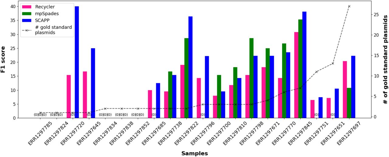
F1 scores of the plasmids assembled by Recycler, mpSpades and SCAPP in human gut microbiome samples, calculated using PLSDB plasmids as the gold standard. The dashed line shows the number of gold standard plasmids in each sample.
4.3 Human gut plasmidome
The human gut microbiome from a fecal sample of a healthy adult male was extracted, enriched for plasmids and sequenced following the protocol outlined in Brown Kav et al. (2013) (approved by local ethics committee of Clalit HMO, approval number 0266-15-SOR). This protocol was assessed to achieve samples with at least 65% plasmid contents by Krawczyk et al. (2018).
We determined the gold standard set of plasmids as in the gut microbiome samples, resulting in 74 plasmids with > 90% of their length covered. Performance was computed as for the metagenomic samples and is shown in Table 2. mpSpades had lower precision and much lower recall than the other tools. SCAPP achieved better overall performance as a result of higher precision.
Performance on the human gut plasmidome.
Notably, though the sample was obtained from a healthy donor, some of the reconstructed plasmids matched reference plasmids annotated with virulence-associated hosts such as Klebsiella pneumoniae, pathogenic serovars of Salmonella enterica, and Shigella sonnei. The detection of plasmids previously isolated in pathogenic hosts in bacteria in the healthy gut indicates potential pathways for transfer of virulence genes.
We used MetaGeneMark (Zhu et al., 2010) to find potential genes in the plasmids assembled by SCAPP (294 genes) and then annotated them with the NCBI non-redundant (nr) protein database. 46 of the plasmids contained 170 (58%) annotated genes, of which 77 (45%) had known functional annotations, which we grouped manually in Figure 3A. There are five antibiotic and toxin resistance genes, all on plasmids that were not in the gold standard set, highlighting SCAPP’s ability to find novel resistance carrying plasmids. Most of the genes with functional annotations are for plasmid functions covering 29 out of 33 of the plasmids with functionally annotated genes (88%). This provides a strong indication that SCAPP succeeded in assembling true plasmids.
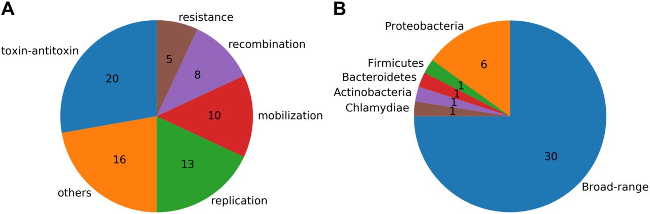
Annotation of genes in the plasmids identified by SCAPP on the human gut plasmidome sample. A) Functional annotations of the plasmid genes. B) Host annotations of the plasmids. Broad-range plasmids had genes annotated with hosts from more than one phylum.
We also examined the hosts that were annotated for the plasmid genes, shown in Figure 3. Almost all of the annotated plasmids had genes that were from a broad range of hosts, defined as being identified in hosts from more than one phylum. This demonstrates the broad host range of many of the plasmids that SCAPP finds and highlights the importance of plasmids in transferring genes, such as the antibiotic resistance genes we detected across a range of bacteria.
4.4 Parallel metagenomic and plasmidome samples
We performed two sequencing assays on the same cow rumen microbiome sample (4 month old calf, approvals by the local ethics committee of the Volcani Center, numbers 412/12IL and 566/15IL). In one subsample we performed metagenomic sequencing. The other subsample underwent plasmid enrichment before sequencing according to the protocol of Brown Kav et al. (2013). (see Figure 6A). This enabled us to assess the plasmids assembled in the metagenome using the plasmidome. Because the plasmidome was from the same sample as the metagenome, it could provide a better assessment of performance than using PLSDB matches as the gold standard, especially as PLSDB tends to under-represent plasmids in non-clinical contexts.

Comparison of the plasmids assembled by each tool. A) Overlap between plasmids found in the metagenomic sample. B) Overlap between plasmids found in the plasmidomic sample.

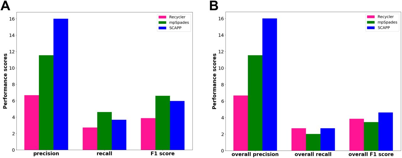
Performance on the parallel dataset. A) Precision, recall and F1 score of each tool on the plasmids assembled from the metagenome compared to the plasmids assembled from the plasmidome. B) Overall precision, recall, F1 score of the tools on the plasmids assembled from the metagenome compared to the union of all plasmids assembled by all tools in the plasmidome.

Using the plasmidome reads to evaluate the quality of metagenome assembly. A) Plasmidome (I) and metagenome reads (II) are obtained from subsamples of the same sample. III: The metagenome reads are assembled into a graph. IV: The graph is used to detect and report plasmid by the algorithm of choice. V. The plasmidome reads are matched to assembled plasmids. Nearly fully matched plasmids (red) are used to calculate plasmid read-based precision. VI. The plasmidome reads are matched to the assembly graph contigs. Nearly fully covered contigs (red) are considered plasmidic. The fraction of total length of plasmidic contigs included in the detected plasmids gives the plasmidome read-based recall. B) Plasmidome read-based performance.
We ran the three plasmid discovery algorithms on each of the subsamples. The results are presented in Table 3. In both subsamples, mpSpades made the least predictions and Recylcer made the most. To compare the plasmids identified by the different tools, we considered two plasmids to be the same if their sequences matched at > 80% identity across > 90% of their length. The comparison is shown in Figure 4. On the plasmidome subsample, fifty one plasmids were identified by all three methods. Seventeen were common to the three methods in the metagenome. In both subsamples, the Recycler plasmids included almost all those identified by each of the other two methods and also a large number of additional plasmids. In the plasmidome, SCAPP and Recycler shared many more plasmids than mpSpades and Recycler.
Number of plasmids assembled by each tool and their median lengths (in kbp) for the parallel metagenome and plasmidome samples.
Comparison of the assemblies to PLSDB (as was done for the human gut samples) gave very few results. The metagenome contained only one matching PLSDB reference plasmid, and none of the tools assembled it. The plasmidome had only seven PLSDB matches, and mpSpades, Recycler, and SCAPP had F1 scores of 2.86, 2.67, and 1.74, respectively. The low numbers of PLSDB matches compared to the number of plasmids assembled demonstrate the ability of the tools to identify novel plasmids that are not in the database.
We next compared the plasmids assembled by each tool in the two subsamples. For each tool, we considered the plasmids it assembled from the plasmidome to be the gold standard set, and computed scores as above for the plasmids it reported for the metagenome. The results are presented in Figure 5A. SCAPP had the highest precision. Since mpSpades had a much smaller gold standard set, it achieved higher recall and F1. Recycler output many more plasmids than the other tools in both samples, but had much lower precision, suggesting that many are spurious.
Next, we considered the union of the plasmids assembled across all tools to be the gold standard set and recomputed the scores as before. We refer to them as the “overall” scores. The results in Figure 5B show that overall precision scores were the same as in Figure 5A, while overall recall was lower for all the tools. mpSpades underperformed because of its smaller set of plasmids and SCAPP had the highest overall F1 score.
Finally, in order to fully leverage the power of parallel samples, we computed the performance of each tool on the metagenomic sample, using the reads of the plasmidomic sample, and not just the plasmids that the tools were able to assemble. We calculated the plasmidome read-based precision by mapping the plasmidomic reads to the plasmids assembled from the metagenomic sample (Figure 6A). A plasmid with > 90% of its length covered by more than one plasmidomic read was considered to be a true positive. The plasmidome read-based recall was computed by mapping the plasmidomic reads to the contigs of the metagenomic assembly. Contigs with > 90% of their length covered by plasmidomic reads at depth > 1 were considered to be plasmidic. Plasmidic contigs that were integrated into the assembled plasmids were counted as true positives, and those that were not were considered false negatives. The recall was the total fraction of the plasmid contigs that was covered by integrated contigs. Note that the precision and recall here are measured using different units (plasmids and base pairs, respectively) so they are not directly related. For mpSpades, which does not output a metagenomic assembly, we mapped the contigs from the metaSPAdes assembly to the mpSpades plasmids using BLAST (> 80% sequence identity matches along > 90% of the length of the contigs).
The pasmidome read-based performance is presented in Figure 6B. All tools achieved a similar recall of around 12. SCAPP and mpSpades performed very similarly, with SCAPP having slightly higher precision (24.0 vs 23.1) but slightly lower recall (11.9 vs 12.2). Recycler had a bit higher recall (13.1), at the cost of much lower precision (11.7). Hence, a much lower fraction of the plasmids assembled by Recycler in the metagenome are actually supported by the parallel plasmidome sample, adding to the other evidence that Recycler makes many more false positive calls than the other tools.
We assessed the significance of the improved plasmid assembly by SCAPP. Only one plasmid in PLSDB was covered by contigs in the metagenomic assembly, demonstrating the ability of SCAPP to identify novel plasmids that are not in the databases. Four of the plasmids assembled by SCAPP in the metagenome sample were also assembled with the same sequence in the plasmidome sample.
There were 293 contigs in the metagenomic assembly that were covered by plasmidomic reads, with a total length of 146.6 kbp. 17.4 kbp of this length were incorporated into plasmids assembled by SCAPP. In contrast, the plasmidome assembly had a total length of 8.9 Mbp. This clearly shows the potential advantage of plasmidome sequencing for determining plasmids. This is also apparent from the low recall seen in Figure 5A.
We detected potential genes in the plasmids assembled by SCAPP in the plasmidome sample and annotated them as we did for the human gut plasmidome. Out of 242 genes, only 34 genes from 17 of the plasmids had annotations, and only 18 of these had known functions, highlighting that many of the plasmids in the cow rumen plasmidome are as yet unknown. These functions are shown in Figure 7A. The high concentration of genes of plasmid function indicates that SCAPP succeeded in assembling novel plasmids. Unlike in the human plasmidome, most of the plasmids with known host annotations have hosts from a single phylum, see Figure 7B.

Annotation of genes in the plasmids identified by SCAPP on the rumen plasmidome sample. A) Functional annotations of the plasmid genes. B) Host annotations of the plasmids.
4.5 Summary
We summarize in Table 4 the performance of the tools across all the datasets. We say the per-formance of two tools is similar (denoted ≈) if their scores are within 5% of each other, and that one has much higher performance than the other (≫) if its score is > 30% more. Unless otherwise stated, F1 score is used.
Summary of performance. Comparison of the performance of the tools on each of the datasets. When multiple samples were tested, the number of samples appears in parentheses, and average performance is reported. For the parallel samples results are for the evaluation of the metagenome based on the plasmidome.
We see that in most cases SCAPP is the highest performing, and other than in the case of the small simulations, SCAPP performs close to the top performing tool.
4.6 Resource usage
We compared the runtime and memory usage of the three tools, presented in 5. Recycler and SCAPP require assembly by metaSPAdes and pre-processing of the reads and resulting assembly graph. SCAPP also requires post-processing of the assembled plasmids. mpSpades requires post-processing of the assembled plasmids with the plasmidVerify tool. The reported runtimes are for the full pipelines necessary to run each tool – from reads to assembled plasmids.
In almost all cases assembly was the most memory intensive step, with metaSPAdes and mpSpades reaching very similar peak RAM usage (within 0.01 GB), and so we report the RAM usage for this step. The assembly step was also the longest step in all cases.
The runtimes and memory usage for each of the tools are shown in Table 5. Performance measurements were made on a 44-core, 2.2 GHz server with 792 GB of RAM. 16 processes were used where possible. Recycler is single-threaded, so only one process could be used for that step. Note that mpSpades does not output a metagenomic assembly graph, so users interested in both the plasmid and non-plasmid sequences in a sample would need to run metaSPAdes as well, practically doubling the runtime.
Resource usage comparison for the three methods. Peak RAM of the assembly step (metaSPAdes for Recycler and SCAPP, metaplasmidSPAdes for mpSpades) in GB. Runtime (wall clock time, in minutes) is reported for the entire pipeline including assembly and any pre-processing and post-processing required. Metagenome results are an average across the 20 samples.
5 Conclusion
Plasmid assembly from metagenomic sequencing is extremely difficult as seen by the low numbers of plasmids found in real samples. This is true even in samples of the human gut microbiome, which is widely studied – relatively few plasmids from the extensive PLSDB plasmid database were covered in assemblies of these samples. Despite the challenges, SCAPP succeeded in assembling plasmids in real samples. SCAPP demonstrated generally improved performance over Recycler and metaplasmidSPAdes in a wide range of contexts. By applying SCAPP across large sets of samples, many new plasmid reference sequences can be assembled, enhancing our understanding of plasmid biology and ecology.
Funding
PhD fellowships from the Edmond J. Safra Center for Bioinformatics at Tel-Aviv University and Israel Ministry of Immigrant Absorption (to DP). Israel Science Foundation (ISF) grant 1339/18, US - Israel Binational Science Foundation (BSF) and US National Science Foundation (NSF) grant 2016694 (to RS), ISF grant 1947/19 and ERC Horizon 2020 research and innovation program grant 640384 (to IM).
Supplementary information
S1 Plasmid-specific genes
We used five sets of plasmid-specific genes:
MOB genes 1: 331 amino acid sequences of plasmid maintenance genes curated by plasmid biologists and filtered computationally (see details of filtering below).
MOB genes 2: Larger set of 559 amino acid sequences of plasmid maintenance genes curated by plasmid biologists and filtered computationally.
Plasmid ORFs: 4276 nucleotide sequences corresponding to ORFs annotated with ‘mobilization’, ‘conjugation’, ‘partitioning’, ‘toxin-antitoxin’, ‘replication’, or ‘recombination’ from a large set of putative plasmids found by the Mizrahi Lab and then filtered computationally.
ACLAME plasmid genes: 4813 nucleotide sequences of genes that make up 96 gene families in the ACLAME (Leplae et al., 2009) database that were manually selected as being possibly plasmid-specific. The set of genes was deduplicated and filtered computationally.
PLSDB-specific ORFs: 94478 plasmid-specific sequences determined as follows: We used MetaGeneMark (Zhu et al., 2010) to predict genes in the plasmid sequences from PLSDB (v.2018 12 05) (Galata et al., 2018). We then counted the number of BLAST matches (> 75% identity match along > 75% of the gene length) to these genes in both PLSDB and bacterial reference genomes from NCBI (downloaded January 9, 2019). We considered each predicted gene that appeared in the plasmids more than 20 times and was > 20× more prevalent in the plasmids than in the genomes to be plasmid-specific.
Sets 1–4 were filtered as follows: We counted matches between the sequences and PLSDB plasmids and NCBI bacterial reference genomes as for the PLSDB-specific ORFs (set 5). We excluded any gene that had more than 4 matches to bacterial genes and met one of the following conditions: (1) ≤ 4 matches to plasmid genes and > 4× as many matches to bacterial genes as plasmid genes; or, (2) > 4 plasmid gene matches, but ≤ 4× as many matches to plasmid genes as to bacterial genes.
All of these gene sets are available in the SCAPP release from https://github.com/Shamir-Lab/SCAPP/data in the following locations:
MOB genes 1: aa/aa2
MOB genes 2: aa/aa1
Plasmid ORFs: nt/nt3
ACLAME plasmid genes: nt/nt1
PLSDB-specific ORFs: nt/nt2
S2 The SCAPP algorithm
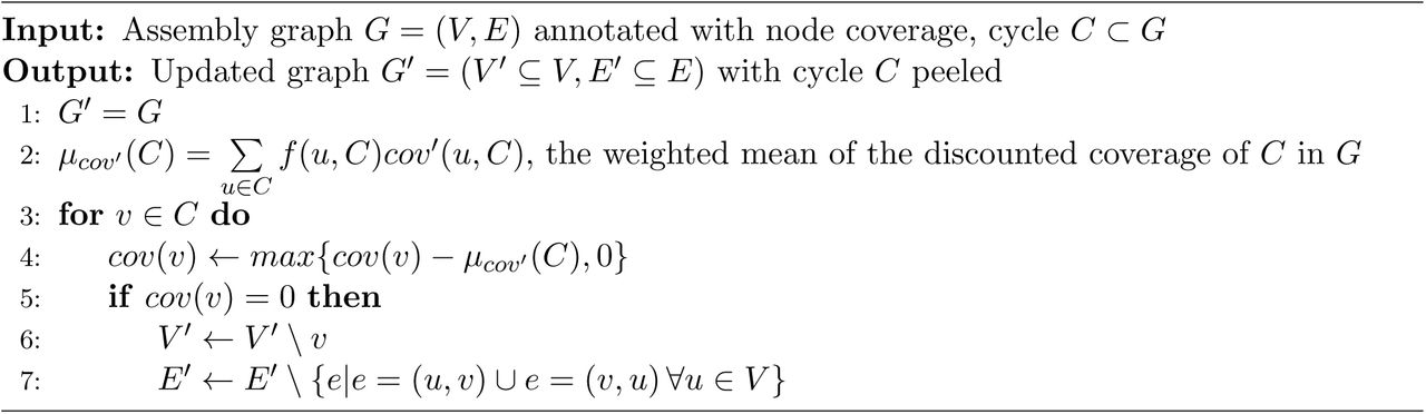
The full SCAPP algorithm is detailed in Algorithm 1. The helper function peel(G, C) which defines how cycle C is peeled from the graph is given in Algorithm 2.
S3 List of real human gut microbiome samples
The accessions of the publicly available human metagenomic samples assembled are:

S4 Software documentation
SCAPP is fully documented at https://github.com/Shamir-Lab/SCAPP. We outline the installation and usage instructions here.
S4.1 Installing SCAPP
SCAPP is written in Python3 and requires a number of packages which will be installed by the setup script.
SCAPP requires BWA, the NCBI BLAST+ executables, and samtools. We also highly recommend installing PlasClass to use full functionality of the SCAPP pipeline (available from: https://github.com/Shamir-Lab/SCAPP).
To install PlasClass do:
git clone https://github.com/Shamir-Lab/SCAPP.git cd SCAPP python setup.py installWe recommend using a virtual environment.
S4.2 Configuring SCAPP paths
SCAPP requires configuration variables specifying the paths to the BWA, BLAST+, and samtools executables for the system it is being run on.
Set the paths to these executables in the file bin/config.json.
This information can be configured once when first installing SCAPP and then used for all SCAPP runs provided the locations of those executables do not change.
Alternatively, the locations of these executables can be added to the PATH environment variable. If these executables are in the PATH environment variable so that they can be run from any location on the system without specifying the path, then the SCAPP configuration variables can be left blank and there is no need to alter the file config.json.
S4.3 Running SCAPP: Basic Usage
SCAPP is run using the script SCAPP.py in the bin directory as follows: python scapp.py -g <assembly graph> -o <output directory> -k <max k value> -r1 <reads 1> -r2 <reads 2>
If a BAM file aligning the reads to assembly graph nodes already exists (for example from a previous run of SCAPP), then the BAM file can be used instead of the reads files rather than having the pipeline redo the alignment: python scapp.py -g <assembly graph> -o <output directory> -k <max k value> -b <BAM>
The basic command line options are:
-g/--graph: Assembly graph fastg file.
-o/--output_dir: Output directory.
-k/--max_k: Maximum k value used by the assembler. Default: 55.
-p/--num_processes: Number of processes to use. Default: 16.
-r1/--reads1: Paired-end reads file 1.
-r2/--reads2: Paired-end reads file 2.
-b/--bam: BAM alignment file aligning reads to graph nodes. -b and -r1,-r2 are mutually exclusive.
The -g, -o and either -r1,-r2 or -b options are required for every run of SCAPP.
S4.4 SCAPP output files
SCAPP creates a number of subdirectories and outputs files in the output directory specified by the user. Key output files are highlighted:
The primary output is the file <prefix>.confident_cycs.fasta which contains the confident plasmid predictions (prefix is the name of the input assembly graph file less the suffix).
The scapp.log file contains a log of the SCAPP run.
<prefix>.cycs.fasta contains all the potential plasmids – cycles that pass the cycle criteria. The confident cycles that are predicted as plasmids are a subset of these. Users may want to examine these potential plasmids.
<prefix>.cycs.paths.txt contains the paths for each potential plasmid. The name of the plasmid is listed. On the next line, the names of the set of edges that are contained in the cycle are listed in order. The third line for each entry lists the numbers of those edges (for easier use with visualisation tools).
The files reads_pe_primary.sort.bam, reads_pe_primary.sort.bam.bai, and plasclass.out contain the outputs of preprocessing steps in the SCAPP pipeline. These steps are the most time consuming, and the files can be passed into the pipeline (using the -b and -pc parameters) in order to skip these steps in case SCAPP is run multiple times on the same sample.
S4.5 Advanced options
The SCAPP pipeline is configurable and there are many advanced options to set different thresholds and inputs in the algorithm. In most cases, we advise using the default settings and pipeline configurations.
There are a number of ways the stages of the SCAPP can be modified with the following parameters:
-sc/--use_scores: Flag to determine whether to use plasmid scores. Use value False to turn off plasmid score use. Default True.
-gh/--use_gene_hits: Flag to determine whether to use plasmid specific genes. Use value
False to turn off plasmid gene use. Default True.
-pc/--plasclass: PlasClass score file. If PlasClass classification of the assembly graph nodes has already been performed, provide the name of the PlasClass output file.
-pf/--plasflow: PlasFlow score file. To use PlasFlow scores for the nodes instead of Plas-Class, provide the name of the PlasFlow output file. -pf, -pc are mutually exclusive.
The following parameters change thresholds used in the algorithm:
-m/--max_CV: Maximum allowed coefficient of variation for coverage. Default: 0.5.
-l/--min_length: Minimum allowed length for potential plasmid. Default: 1000.
-clft/--classification_thresh: Threshold for classifying a potential plasmid as a plasmid. Default: 0.5.
-gm/--gene_match_thresh: Threshold for % identity and fraction of length covered to determine plasmid gene matches. Default: 0.75.
-sls/selfloop_score_thresh: Threshold plasmid score above which a self-loop is considered a potential plasmid. Default: 0.9.
-slm/--selfloop_mate_thresh: Threshold fraction of off-loop mate-pairs, below which a self-loop is considered a potential plasmid. Default: 0.1.
-cst/--chromosome_score_thresh: Threshold score, below which a long node is considered a chromosome node. Default: 0.2.
-clt/--chromosome_length_thresh: Threshold length, above which a low scoring node is considered a chromosome node. Default: 10000.
-pst/--plasmid_score_thresh: Threshold score, above which a long node is considered a plasmid node. Default: 0.9.
-plt/--plasmid_length_thresh: Threshold length, above which a high scoring node is considered a plasmid node. Default: 10000.
-cd/--good_cyc_dominated_thresh: Threshold for the maximum fraction of nodes with most mate-pairs off the cycle allowed for the cycle to be considered a potential plasmid. Default: 0.5.
Note that instead of setting each of these parameters on the command line, they can instead be set using the file bin/params.json. Simply set each variable in this file to the desired value and it will be used in SCAPP. Any value passed as a command-line parameter will override the values set in this file.
Acknowledgements
We thank members of the Shamir Lab for their help and advice – Roye Rozov, Hagai Levi, Lianrong Pu, and Nimrod Rappoport.


