

Abstract
Freshwater ecosystems are experiencing greater variability due to human activities, necessitating new tools to anticipate future water quality. In response, we developed and operationalized a near-term iterative water temperature forecasting system (FLARE – Forecasting Lake And Reservoir Ecosystems) that is generalizable for lakes and reservoirs. FLARE is composed of: water quality and meteorology sensors that wirelessly stream data, a data assimilation algorithm that uses sensor observations to update predictions from a hydrodynamic model and calibrate model parameters, and an ensemble-based forecasting algorithm to generate forecasts that include uncertainty. Importantly, FLARE quantifies the contribution of different sources of uncertainty (parameters, driver data, initial conditions, and process) to each daily forecast of water temperature at multiple depths. We applied FLARE to a temperate reservoir during a 100-day period that encompassed stratified and mixed thermal conditions and found that daily forecasted water temperatures were on average within 0.91℃ at all depths of the reservoir over a 16-day forecast horizon. FLARE successfully predicted the onset of fall turnover eight days in advance, and identified meteorology driver data and downscaling as the dominant sources of forecast uncertainty. Overall, FLARE provides an open-source and easily-generalizable system for water quality forecasting for lakes and reservoirs to improve management.
Key Points
We created a near-term iterative lake water temperature forecasting system that uses sensors, data assimilation, and hydrodynamic modeling
FLARE quantifies the uncertainty in each daily forecast and provides an open-source, generalizable system for water quality forecasting
16-day forecasted temperatures were within 0.91°C over 100 days in a reservoir case study
1 Introduction
As a result of human activities, ecosystems around the globe are increasingly changing [Stocker et al. 2013, Ummenhofer and Meehl 2017], making it challenging for resource managers to consistently provision vital ecosystem services [West et al. 2009]. In particular, managers of freshwater ecosystems, which have been more degraded than any other ecosystem on the planet [Millennium Ecosystem Assessment 2005], are seeking new tools to anticipate future change and ensure clean water for drinking, fisheries, irrigation, industry, and recreation [Brookes et al. 2014].
In response to this need, near-term iterative ecological forecasting has emerged as a solution to provide stakeholders, managers, and policy-makers crucial information about future ecosystem conditions [Clark et al. 2001, Dietze et al. 2018, Luo et al. 2011]. Here, we define a near-term iterative forecast as a projection of future ecosystem states with fully-specified uncertainties, generated from predictive models that can be constantly updated with new data as they become available [Clark et al. 2001]. Importantly, a near-term iterative forecast is not created from merely one ecosystem simulation, but an ensemble of simulations that enable quantification of the uncertainty in the forecast contributed by different sources [i.e., parameters, driver data, initial conditions, and process; Dietze 2017a, Dietze 2017b]. Because quantifying the sources of forecast uncertainty is a major goal of ecological forecasting research, multiple approaches have been developed to estimate and reduce forecast uncertainty [e.g., Bayesian state-space modeling, particle filters, and ensemble filters; Dietze 2017a]. Fully-specified uncertainty provides both an assessment of confidence in a forecast for managers as they interpret the forecasts for decision-making and valuable information for researchers about how to improve forecasts.
Forecasts of water temperature are particularly valuable for managers that oversee drinking water supply lakes and reservoirs, as waterbody temperatures can be very dynamic due to meteorological forcing, management, and seasonality [e.g., Klug et al. 2012, Mi et al. 2019, Schmidt et al. 2018, Sharma et al. 2015]. Because water temperature is closely related to many water quality metrics, including microbial and algal growth, dissolved oxygen saturation, the release of chemical constituents from sediments into the water column, and habitat suitability for organisms [e.g., fish; Butcher et al. 2015, Carey et al. 2012, Delpla et al. 2009, Jöhnk et al. 2008], water temperature profile data are used to determine withdrawal depths for water treatment, extraction schedules for hydropower generation, and in situ water quality management [Çalışkan and Elçi 2008, Casamitjana et al. 2003, Weber et al. 2017]. Water temperature depth profiles also determine the strength of thermal stratification, i.e., if there are discrete epilimnetic (surface) and hypolimnetic (bottom) layers or isothermal (fully-mixed) conditions [Read et al. 2011]. When waterbodies transition from stratified to mixed conditions during the onset of fall turnover, reduced nutrients and metals that accumulated in the hypolimnion during the summer are mixed throughout the water column, decreasing water quality [Cooke et al. 2005, Effler and Matthews 2008]. Consequently, near-term iterative forecasts of water temperature profiles would allow managers to preemptively respond to impending poor water quality during fall turnover and other episodic events (e.g., storms) that alter water temperature and thermal stratification.
Here, we introduce a forecasting system (FLARE, Forecasting Lake And Reservoir Ecosystems) that generates automated 16-day water temperature forecasts and is generalizable to many lakes and reservoirs (Figure 1). FLARE is composed of: 1) water quality and meteorology sensors deployed in a lake or reservoir that wirelessly stream data, 2) a data assimilation algorithm that uses sensor observations to update water temperature predictions from a hydrodynamic model and to calibrate model parameters, and 3) an ensemble-based forecasting algorithm to generate forecasts that quantify the sources of forecast uncertainty. FLARE quantifies uncertainty from model process (i.e., the capacity of a calibrated model to reproduce past observations), model parameters, initial conditions (i.e., the uncertainty observed in water temperatures on the first day of the forecast), and driver data (i.e., the uncertainty in future weather forecasts that are needed to run the hydrodynamic model). The forecasting system samples from these sources of uncertainty to generate probability distributions for water temperature at multiple depths and can generate probability distributions of hydrodynamic events such as the occurrence of fall turnover.
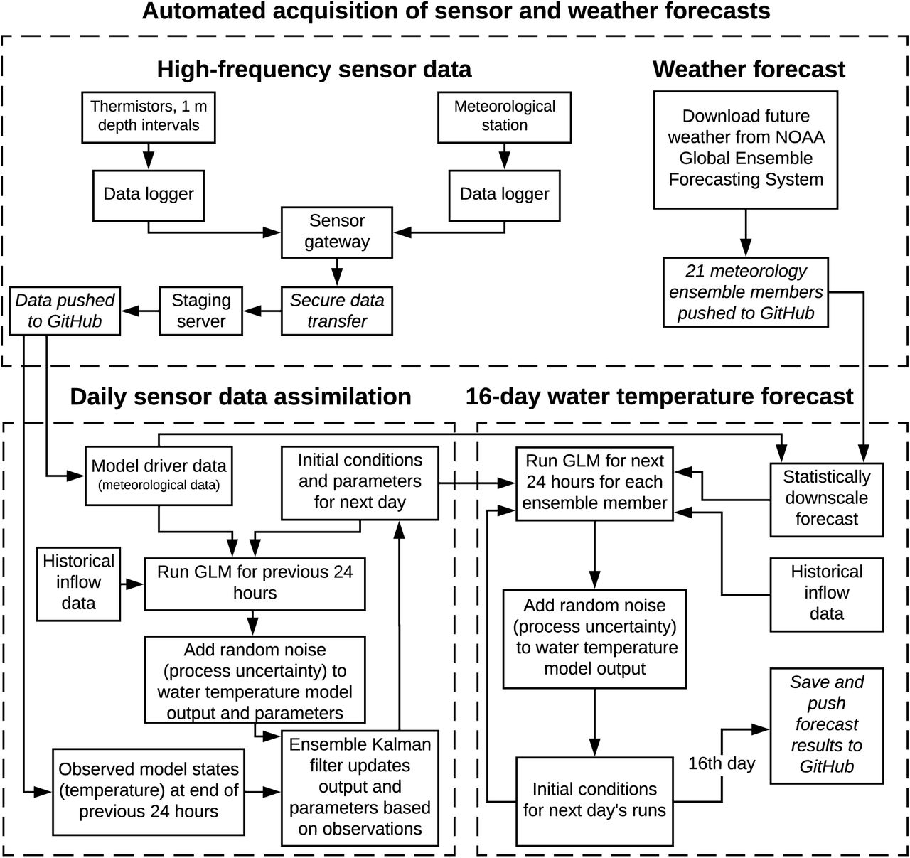
A conceptual diagram describing the data assimilation and forecasting workflow for the FLARE (Forecasting Lake And Reservoir Ecosystems) system. The high-frequency sensor data and NOAA 16-day weather forecasts are transferred to a GitHub repository where the data assimilation algorithm uses the output of the previous day’s data assimilation as initial conditions for the current day, assimilates the new sensor observations to update water temperature predictions and model parameters, and passes the updated temperatures and parameters to the forecasting algorithm as initial conditions for generating predictions of future ecosystem states with their uncertainty. The forecasting system spatially and temporally downscales the 16-day NOAA Global Ensemble Forecasting System forecasts to local site conditions at the hourly scale and propagates the process uncertainty through the 16-day forecast horizon.
We set up the forecasting system to automatically generate probabilistic water temperature forecasts for a drinking water reservoir over 100 days to address the following questions: 1) How does forecasting performance differ among three key stages of lake thermal dynamics (summer stratification, fall turnover, and fall mixing)?, 2) How well does the forecasting system predict the onset of fall turnover?, and 3) What are the contributions of different sources of uncertainty to the forecasts?
2 Methods
We developed a forecasting system (FLARE; Forecasting Lake And Reservoir Ecosystems) that predicts water temperature at any set of specified depths in a lake or reservoir for a 16-day time horizon using a physics-based hydrodynamic model. The system uses observed data and data assimilation techniques to generate the initial conditions, parameters, and uncertainty estimates for a forecast into a 16-day future. We describe the forecasting methods below and the data assimilation methods in Supporting Information A.
2.1 Hydrodynamic model
FLARE simulated reservoir hydrodynamics with the General Lake Model (GLM), a one-dimensional (1-D) vertical stratification model [Hipsey et al. 2019]. We used GLM because: 1) the model has successfully reproduced observed water temperature profiles in lakes around the world with varying mixing regime, climate, and morphology [Bruce et al. 2018]; 2) GLM is an open-source, community-developed model and thus scalable to other waterbodies for future forecasting applications [Snortheim et al. 2017]; and 3) GLM has low computational needs, enabling many model ensemble members to be run quickly and efficiently, a requirement for near-term iterative forecasting.
To enable generalization to other lakes or reservoirs, we set all but three highly sensitive parameter values equal to the values reported in the default GLM version 3.0 model [Hipsey et al. 2019]. The three parameters, selected using the methods described in Supplemental Information A), were: a scalar for incoming shortwave radiation (sw_factor) and two parameters defining the sediment temperature in the deep and shallow reservoir zones (zone1temp: 5 – 9.3 m deep; zone2temp: 0 – 5 m deep). For driver data, GLM requires hourly meteorological data on downwelling shortwave radiation (W m-2), downwelling longwave radiation (W m-2), air temperature (℃), wind speed (m s-1), relative humidity (%), and precipitation (m day-1) as well as daily rates of water inflow (m3 day-1), inflow temperature (℃), and daily rates of outflow (m3 day-1) [Hipsey et al. 2019].
2.2 Ensemble forecasting approach
The FLARE system uses an ensemble approach to numerically simulate and propagate forecast uncertainty into the future. The ensemble forecasting is based on eqn. 1:
 where G() is the GLM model that requires a vector of water temperatures at the modeled depths as initial conditions
  , a vector of the four calibrated model parameters
  , and a set of model drivers (i.e., weather, inflows, and outflows). The index i in eqn. 1 represents the ith ensemble member and the subscript f is the day in the future (e.g., if f=1, this would be referring to tomorrow). The t subscript denotes the time step in the daily in the data assimilation. MVN is the multivariate normal distribution with a mean of zero and a covariance matrix of Σt.
The contribution of process uncertainty to the total forecast uncertainty is represented by adding a multivariate normal random variable to the GLM predictions (MVN(0, Σt) in eqn 1). This process uncertainty is centered on zero with a covariance matrix (Σt) that represents the uncertainty at each depth (the diagonals of Σt) and the covariance of uncertainty between depths (the off-diagonals of Σt). Σt is calculated from the residuals in the data assimilation before the states were updated using the observations. Eqn. 1 is applied at the daily time step and the random process uncertainty is added each day of the forecast. In eqn. 1, the subscript t on Σt signifies that the covariance matrix does not change through the forecast because t does not incrementally increase when forecasting into the future (t only increments in the daily data assimilation that sets the initial conditions, parameters, and process uncertainty for the forecast).
The 16-day forecasts require initial conditions of the water temperature at each modeled depth ( , where t equals the time step of the data assimilation when the forecast into the future was initialized) and initial model parameters
  on day 0 (f = 0) of the forecast. The variance in xt and αt across ensemble members when the forecast was initialized represents the contribution of initial conditions and parameters, respectively, to the total forecast uncertainty. To generate these initial conditions while also calibrating the three focal parameters, FLARE assimilates temperature sensor observations from the previous day into the GLM using an Ensemble Kalman Filter [EnKF; Evensen 2003, Evensen 2009]. We used data assimilation rather than simply specifying the initial conditions from the observations because the EnKF: 1) enabled the generation of initial conditions when sensor data were not available (e.g., during maintenance), 2) mechanistically-interpolated water temperature between sensor depths, 3) enabled the calibration of model parameters, and 4) generated a historical data product of water temperature with spatial and temporal gap-filling. The EnKF method of data assimilation is well-suited for non-linear mechanistic models like the GLM and enables ensemble-based forecasts of future states [Dietze 2017a]. Our implementation of the EnKF with state augmentation to calibrate parameters (Supporting Information A) follows Zhang et al. (2017).
To quantify the contribution of future meteorological conditions to the total forecast uncertainty, each water temperature ensemble member was assigned one of the ensemble members from the National Oceanic and Atmospheric Administration Global Ensemble Forecasting System (NOAA GEFS). NOAA GEFS provides 21 different modeled representations of future weather conditions at a 16-day time horizon. Each day that a forecast was generated, we downloaded the meteorological driver data required by the GLM from NOAA GEFS for the 0:00:00 UTC forecast using the rNOMADS package in R [Bowman 2019].
Additionally, our forecasts included the uncertainty in temporally and spatially-downscaling the gridded NOAA GEFS meteorological forecasts. NOAA GEFS forecasts were available for 6-hour periods over a 16-day horizon at a 1×1° spatial resolution, which needed to be translated into hourly meteorology driver data for GLM that was specific to local site conditions. Detailed information on the meteorology downscaling are available in Supporting Information B and summarized here. First, we estimated the linear relationship between the daily mean observed value for a variable (e.g., daily mean air temperature) and the mean of the NOAA GEFS ensemble on the 1st day of the NOAA GEFS forecast. We used observations between April 4, 2018 and December 6, 2018 in the linear regression. Second, we calculated the residuals in the linear regression for each day and meteorological variable. Third, we calculated the covariance matrix in the residuals among the meteorological variables. Fourth, to propagate the uncertainty in the downscaling process for the meteorology variables, we sampled from a multivariate distribution with the mean equal to a vector of daily means for the meteorology variables from a NOAA GEFS forecast ensemble member and the covariance equal to the covariance of residuals described above. We repeated the sampling from the multivariate distribution for each day within each NOAA GEFS ensemble member, resulting in an ensemble of meteorological drivers that represented both NOAA GEFS forecast and downscaling uncertainty. For example, 21 draws from this multivariate distribution for each of the 21 NOAA ensemble members resulted in 441 unique ensemble members describing uncertainty in the weather drivers for a particular day in the future. Finally, we converted the daily downscaled value for each meteorological variable to the hourly time resolution needed as model driver data. We used the sub-daily variation inherent in the original 6-hour NOAA forecast to first linearly convert the daily downscaled data to the 6-hour time scale and then second, used a linear spline function to convert the 6-hour data to 1-hour time resolution. In the case of shortwave radiation, we used solar geometry to convert the daily downscaled shortwave radiation to a 1-hour time resolution.
2.3 Application of forecasting system
2.3.1 Site description
We applied and evaluated FLARE at Falling Creek Reservoir (FCR), a dimictic, eutrophic reservoir located in Vinton, Virginia, USA (37.30°N,79.84°W). FCR is a shallow (maximum depth=9.3 m, mean depth=4 m), small (surface area=0.119 km2) reservoir [Chen et al. 2018]. The lake exhibits summer thermal stratification from May to October and is ice-covered from January to February or March [Carey et al. 2019c]. FCR is primarily fed by one upstream tributary and was maintained at full pond throughout this study by the Western Virginia Water Authority (WVWA), who own and manage the reservoir as a drinking water supply [Gerling et al. 2014, Gerling et al. 2016].
We monitored FCR water temperature [Carey et al. 2019b] and meteorology [Carey et al. 2019a] with high-frequency sensors during 11 July to 19 December 2018 and measured the inflow discharge rate of the primary tributary entering FCR through a weir [Carey et al. 2018]. Descriptions of the sensor array and methods for real-time wireless transfer of data to cloud storage are in Supporting Information C. Because we were unable to wirelessly connect the weir sensor to the cloud to transmit the inflow data in real-time, we averaged the previous five years’ data measured on a given day to serve as inflow driver data for forecasting.
2.3.2 Description of forecasting analysis
Our application of the forecasting system was divided into two periods: the spin-up period and the forecasting period. The spin-up period was from 11 July to 25 August 2018 and was used to develop the Σt process uncertainty covariance matrix and to constrain the three parameters that were calibrated using the EnKF. In this period, the EnKF was used to update the states and parameters using observed meteorology as the drivers. We used N=441 ensemble members in the EnKF so that each ensemble member can be associated with one of the 441 weather ensemble members when forecasting (e.g., 21 NOAA GEFS ensemble members each with 21 downscaling ensemble members). We modeled water temperature on 0.33-m depth intervals starting at the surface at 0.1 m through 9.3 m at the sediments. This resulted in 29 model states of water temperature depths in the x matrix (eqn. 1). We had sensor observations for 10 of the 29 model depths (0.1, 1, 2, 3, 4, 5, 6, 7, 8, and 9 m; Supporting Information C).
The second period was the forecasting period when 16-day forecasts were generated each day between 26 August and 3 December 2018. The 100 daily forecasts developed over this period included summer stratified, fall turnover, and fall mixed conditions in the reservoir. During this period, the model states and parameters were advanced one day using observed meteorology and updated using the EnKF. These updated states and parameters were used as the initial conditions for each 16-day forecast, which started at midnight of the current day.
2.3.3 Evaluation of forecasts
We evaluated the forecasts using three metrics that assessed the skill, bias, and quality of confidence intervals. Skill was assessed using the root mean square error (RMSE) of the mean forecasted water temperature and the observed water temperature at each day in the 16-day forecast horizon. Bias was assessed using the absolute difference between the mean forecasted water temperature and the observed water temperature at each day in the 16-day forecast. We averaged the RMSE and bias for each day within the 16-day forecast horizon over the 100 forecasts generated between 26 August and 3 December. We compared the forecast RMSE to the RMSE of a null persistence model that assumed water temperature did not change over the 16-day horizon. The quality of the confidence intervals was assessed by calculating the total number of observations contained in a specific confidence interval. We considered a forecast to be well-calibrated if its 90% confidence intervals contained 90% of the observations over the 100 days of forecasts. The confidence interval would be over-confident if fewer than 90% of observations were contained in this interval and would be under-confident if more than 90% observations were contained. We calculated the proportion of observations in the 10, 20, 30, 40, 50, 60, 70, 80, and 90th confidence intervals for 1-day, 7-day, and 16-day time horizons.
We evaluated the ability of the forecasting system to predict the day that fall turnover was first observed at the reservoir. Following McClure et al. [2018], we defined fall turnover as the first day in autumn when water temperatures at 1 m and 8 m depths are within 1℃. In the forecasts prior to turnover, we calculated the proportion of ensemble members that predicted the 1 m and 8 m water temperatures to be ≤1℃ different on each day in the forecast. We expected this proportion to increase for the day of turnover relative to other days as the onset of turnover approached.
2.3.4 Partitioning of uncertainty
To compare the contributions of the different sources of forecast uncertainty, we simulated each uncertainty source individually and compared the variance in each source to the variance in the total forecast uncertainty. Initial condition uncertainty was isolated by only including uncertainty in the  on the first day of the forecast – i.e., no process error was added, the mean parameter values were used, and only one NOAA GEFS ensemble member was used without downscaling uncertainty. Additionally, we examined the influence of gaps in high-frequency water temperature sensor data availability on forecast uncertainty by again isolating initial condition uncertainty but only allowing weekly observations to update model states in the EnKF (simulating if only weekly sampling data were available for EnKF updating instead of 10-minute resolution data). In this case, we set initial condition uncertainty equal to the uncertainty in the EnKF after six days without observations.
Model process uncertainty was isolated by sampling from the process uncertainty while initializing all ensemble members with the ensemble mean (removing initial condition uncertainty), using the mean parameter values, and using one member of the NOAA GEFS without downscaling. Parameter uncertainty was isolated in a similar way to process uncertainty.
The meteorological driver data uncertainty was separated into two components. First, the uncertainty in the NOAA forecast was isolated by using the 21 ensemble members without downscaling, process, parameters, and initial conditions uncertainty included. The downscaling uncertainty was isolated by adding downscaling uncertainty to a single NOAA ensemble member while not adding process, parameters, and initial conditions uncertainty.
We repeated the forecasting uncertainty partitioning for three different forecasts (1 September, 18 October, and 1 December) to represent the three different stages of lake thermal dynamics that occurred during the forecasting period.
3. Results
3.1 Observational water temperature data
Falling Creek Reservoir exhibited summer thermal stratification from the beginning of the monitoring period in July until the onset of fall turnover on 21 October, and then remained mixed until the end of December 2018 (Figure 2A). During the summer thermally-stratified period, observed water temperatures at the surface reached up to 29.6°C on 11 July before cooling in mid-September. Fall turnover was preceded by cooling surface water temperatures, which decreased from 25.0°C to 15.2°C in the 14 days prior to 21 October. After turnover, the 1 and 8 m depth thermistors recorded water temperatures that had a mean difference of 0.51°C (±0.4°C, 1 S.D) throughout the fall mixing period.

Water temperature in Falling Creek Reservoir during the spin-up period (11 July – 25 August 2018) and forecasting period (26 August to 3 December 2018). (a) A heat map showing the observed temperatures through the water column for the spin-up period when only data assimilation was used to update model temperatures and parameters and the forecasting period when data assimilation was used and a 16-day forecast was generated each day. White values designate days with missing water temperature sensor data. (b) A comparison of the observed water temperature for two depths (0.1 m: red, 8 m: blue) with the modeled temperature (0.1 m: black, 8 m: gray) following updating with data assimilation. The 95% confidence intervals are shown as dashed lines.
3.2 GLM and ensemble Kalman filter (EnKF) performance
The GLM simulation of water temperature with the daily EnKF parameter and initial condition updating was able to successfully simulate reservoir water temperatures throughout the spin-up period (11 July – 25 August) and forecasting period (26 August – 3 December; Figure 2B). Following daily assimilation of observed water temperature data, the RMSE for the water temperature predicted by GLM at the surface (0.1 m) and 8.0 m depth were both 0.01 °C during the spin-up and forecasting periods. During the forecasting period, these post-assimilation water temperature predictions were used as initial conditions for the 16-day forecasts. There were two 1-day thermistor data gaps due to sensor maintenance in September (Figure 2B) that highlight the value of the EnKF for updating initial conditions when observational data are unavailable. The three GLM parameters were well-constrained by data assimilation (Supporting Information Figure 1).
3.3 Forecast performance
Every day between 26 August and 3 December, the forecasting system generated 16-day forecasts of water temperature for the entire water column, successfully capturing summer stratified, fall turnover, and fall mixed conditions (Figure 3). In general, the forecast accuracy was high throughout the 16-day forecast horizon, with forecasted water temperatures within 0.14°C for 0.1 m and 0.41°C for 8.0 m of observed temperatures throughout August-December, averaged across all forecast time horizons (Figure 4A). Aggregated over the entire forecasting period, the forecast bias for 0.1 m remained consistently low regardless of forecast horizon, while the 8-m forecasts showed a small increase in bias from −0.27°C at the 7-day horizon to −0.41°C at the 16-day horizon (Figure 4A). Forecast skill declined as the forecast horizon increased, though it was notable that the forecasted water temperature consistently had lower RMSE than a null persistence model, especially for 0.1 m temperatures throughout the 16-day horizon (Figure 4B). Forecast confidence intervals generally were well-calibrated, though the forecast confidence at the 16-day horizon for 0.1 m depth tended to have more observations within the 40-80% forecast confidence intervals than expected (Figure 4C).

Forecasts successfully predicted water temperature across different lake thermal conditions (summer stratification, fall turnover, and fall mixing) in Falling Creek Reservoir. The forecasts for water temperature at the surface (0.1 m: a, b, c) and at the bottom of the reservoir (8.0 m: d, e, f) in the three thermal regime periods are shown. The vertical black line designates the day when that particular forecast was initialized. The red circles show sensor observations that were used in the data assimilation prior to the forecast generation and the blue circles show the observations during the forecast horizon and represent an independent assessment of forecast performance with data that were not used in data assimilation. The mean water temperature forecast (solid) and 95% forecast intervals (dashed) from each day’s 441 forecast ensemble members are shown.

Water temperature forecasts for 0.1 m (red) and 8.0 m (blue) had low bias, high skill (relative to a null persistence model), and well-calibrated confidence intervals. (a) The absolute difference between the forecasted and observed water temperatures at two depths averaged across all forecasts generated during the 100-day forecasting period. (b) The root mean squared error (RMSE) of the forecasts at two depths averaged across the entire forecasting period in comparison to a null persistence model. The null model assumed that water temperature did not change over the 16-day forecast horizon. (c) The proportion of observations during the forecasting period that were within the forecast confidence interval that is specified on the x-axis. For example, the 90% forecast confidence interval is the 5th to 95th percentile of the 441 forecast ensemble members and ideally should contain 90% of water temperature observations. Values for 1, 7, and 16-day forecast horizons for the 0.1 m depth are shown.
In a comparison of forecasting performance during the different thermal structure periods, the RMSE for 0.1 m depth water temperature forecasts improved after fall turnover for all forecast horizons, while the forecast bias was generally similar for all depths during the summer stratified and fall mixing periods (Table 1). Surface water temperature forecasts after fall turnover had 41-52% lower RMSE than forecasts before turnover for 1, 7, and 16-day horizons, while RMSE for forecasts at 8.0 m did not substantially vary among forecast horizons (Table 1). Bias at the two depths was similar between stratified and mixed conditions across forecast horizons (Table 1). The proportion of observations within the 90% confidence intervals increased by 2-30% in the post-turnover mixed period for both depths at all forecast horizons, except for 0.1 m depth at the 1-day horizon (Table 1).
Forecast evaluation metrics for the forecasting period before fall turnover (during thermally-stratified conditions) and after fall turnover (during mixed conditions) at the water’s surface (0.1 m) and near-sediment (8 m) depths. RMSE (the root mean squared error between observations and forecasted temperatures); bias (the difference between observations and forecasted temperatures); and the proportion of observations within the 90% confidence intervals (CI) are presented.
The forecasts successfully predicted the onset of fall turnover on 21 October ∼8 days in advance (Figure 5). At two weeks prior to turnover (7 October), the predicted chance of turnover occurring on 18, 19, 20, or 21 October ranged from 31.5-45.1%. By 13 October, the predicted chance of turnover occurring on 21 October increased up to 72.8%, 27.4% higher than any of the other potential days. The chance of turnover on 21 October continued to increase over the following 8 days, while the chance of turnover occurring on the preceding days decreased to below 52% on 18 October.

The forecasting system was able to anticipate the day of fall turnover 8 days in advance. (a) An example of a 16-day forecast starting on 15 October that shows the percentage of forecast ensemble members that predict the difference in temperature between 1 m and 8 m to be less than 1℃ (the operational definition of turnover). The vertical line designates the day when turnover occurred (21 October). (b). The % chance of turnover for a particular day changed over time. For example, the forecast initiated on 6 October shows a relatively low and equal probability of turnover occurring on any day between 18 – 21 October. In subsequent forecasts, the probability of turnover occurring on the date when it was ultimately observed (21 October) separates from the other dates ∼8 days before turnover occurred.
3.4 Uncertainty partitioning
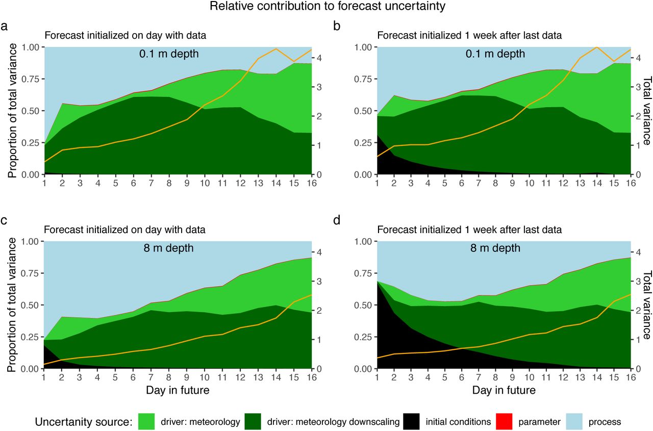
Aggregated over the three 16-day forecasts when uncertainty was partitioned (1 September 1, 18 October, and 1 December), the total forecast uncertainty was approximately two times higher for forecasts at 0.1 m than 8.0 m, but the relative importance of different components to total forecast uncertainty were similar between depths (Figure 6; Supporting Information Figures 2, 3, and 4 show the three forecasts separately). For both depths, the meteorology downscaling uncertainty and NOAA GEFS meteorology driver uncertainty were the largest contributors to the total forecast uncertainty (Figure 6). The meteorology downscaling contribution remained fairly large and constant over time, whereas the meteorology driver data uncertainty grew from near zero at the 7-day horizon to be the largest contributor of uncertainty at the 16-day horizon for the 0.1 m depth and near-equal contributor with meteorology downscaling at the 8.0 m depth. Initial condition uncertainty only contributed to total forecast uncertainty if there was a data gap on the day the forecast was generated, which decreased to near zero at the 8-day horizon for 0.1 m forecasts and the 13 day-horizon for 8.0 m forecasts (Figure 6B,D). As a result of the contributions of each of these components, total uncertainty in the 8.0 m forecasts remained fairly constant for the first 7 days in the forecast and then increased until the end of the 16-day horizon, while the total uncertainty in the 0.1 m forecasts exhibited a linear increase over time.
The relative contribution of the individual sources of uncertainty (left axis) to the total forecast uncertainty (right axis, orange line) varies through the 16-day forecast horizon. The relative contributions and total forecast variance for each day are averaged across the three 16-day forecasts shown in Figure 3: one during summer stratification (Supporting Information Figure 2), one during fall turnover (Supporting Information Figure 3), and one during the fall mixed period (Supporting Information Figure 4). Two depths are shown (0.1 m – a, b; 8.0 m – c, d) and the relative contributions of initial condition uncertainty without (left) and with (right) gaps in water temperature sensor observations are shown in the two columns.
4 Discussion
Overall, FLARE was able to forecast the water temperature on average within 0.91±0.3°C (RMSE±1 S.D.) at all depths of the reservoir over a 16-day horizon during a 100-day period that encompassed both stratified and mixed thermal conditions. Importantly, the forecasting system was able to both predict observed temperatures and identify the transition between stratified and mixed periods with high accuracy. In general, the forecasting system performance was similar between stratified and mixed periods (Table 1), suggesting that the system is likely robust in a range of reservoir conditions, though additional forecasts are necessary to provide a full assessment of FLARE performance. Generally, 1-D hydrodynamic models used for hindcasting aim to predict water temperature within an RMSE of 2°C [e.g., Bruce et al. 2018, Read et al. 2014], so the level of accuracy associated with FLARE future forecasts exceeds expectations.
We found that process uncertainty was the most important source of uncertainty early in the 16-day forecast but that driver data uncertainty dominated by the end of the forecasting period. This finding is consistent between the surface and deep depths at the reservoir and across summer stratified to fall mixed conditions. Importantly, this finding does not mean that process uncertainty declines through the forecast horizon, rather, the total uncertainty grows while the relative importance of process uncertainty diminishes. Within meteorological driver data uncertainty, the role of uncertainty in the NOAA ensemble forecast is comparable to the role of uncertainty in downscaling the coarse-scale NOAA forecast to the local site using data from the meteorological station located at the reservoir. This highlights that future work should focus on evaluating whether more advanced downscaling methods, such as neutral networks [Kumar et al. 2012], can build better relationships between the NOAA forecasts and the local meteorological station.
Our uncertainty results are comparable to Dietze [2017b], who partitioned the uncertainty in net ecosystem exchange carbon flux forecasts in a forest over 16-day horizons. In both studies, the NOAA ensemble driver data uncertainty dominated total forecast uncertainty at the end of the 16-day horizon. Dietze [2017b] found that process uncertainty was more important than the meteorological driver data uncertainty early in the 16-day forecast horizon, though that study did not include NOAA forecast downscaling uncertainty. Overall, while that study [Dietze 2017b] and ours are only two examples of forecast uncertainty partitioning, they do provide insight from very different ecosystems (reservoir water temperatures vs. forest carbon fluxes) and together suggest that meteorological driver data are an important contributor of uncertainty in near-term iterative forecasts.
We found that initial condition uncertainty in the forecasts was relatively small and well-constrained by assimilating high-frequency temperature sensor data using the ensemble Kalman filter. However, high-frequency temperature data are rarely available in real-time for most lakes and reservoirs because of cost and logistics [Marce et al. 2016]. Here, we show that daily iterative forecasting using only weekly observational data to constrain initial conditions increases the role of initial condition uncertainty in the total forecast uncertainty but its role declines to zero through the 16-day forecast horizon. Moreover, the total uncertainty early in the forecast horizon is still low relative to the end of the 16-day horizon regardless of using a daily or weekly water temperature sampling frequency. This highlights that automated temperature sensors may not be a requirement for developing water temperature forecasts, depending the level of acceptable forecast uncertainty over the 1 to 10-day forecast horizon. Thus, it is still possible to generate accurate water temperature forecasts using only manually-collected, weekly temperature profiles.
We anticipate that FLARE may be of interest to managers of other lakes and reservoirs where water temperature forecasts up to 16 days in advance can provide decision support. For Falling Creek Reservoir, an 8-day window to anticipate fall turnover provides sufficient time for managers to buy additional chemicals in preparation for the water quality impairment that occurs during turnover, change staffing schedules, and reprioritize management operations [WVWA, unpubl. data]. Given FCR’s small surface area and shallow depth, it would be expected that the forecasting system would be more accurate in larger, deeper lakes that are less sensitive to meteorological forcing. However, the difference in forecasts generated from the null persistence model and FLARE would likely be smaller in those bigger systems. We anticipate that FLARE would be most useful for managing water bodies that experience dynamic mixing throughout the year and systems where water quality, fish habitat, and reservoir withdrawals are tightly coupled to water temperature.
While the FLARE forecasting system presented here was able to predict water temperature over the 16-day time horizon with low bias and an RSME substantially better than a null persistence model, there are important areas for potential improvement. First, FLARE is using a physics-based, 1-D hydrodynamic model for predictions. Other approaches, such as machine learning or hybrids between machine learning and physics-based models [e.g., Jia et al. 2019], could reduce forecast uncertainty. However, machine learning-based methods must be able to fully quantify forecast uncertainty to be comparable to our process model-based approach. Second, our parameter uncertainty is likely unrealistically low because we only included three parameters in the EnKF data assimilation. While the ability to estimate parameters using EnKF is well-established, the EnKF method is not specifically designed to estimate parameter distributions like Bayesian Monte-Carlo Markov Chain methods [Dietze 2017a]. A current limitation to implementing a Bayesian Monte-Carlo Markov Chain approach is the computation time to execute the GLM simulation within a daily iterative workflow. Future work that uses emulators of GLM may be able to speed computation and allow for more robust estimation of the joint distribution model of parameters that represent both prior knowledge and observed data [e.g., Fer et al. 2018]. Finally, our implementation of FLARE at FCR used historical inflow data in the forecast. Ideally, the forecasts would use a watershed hydrology model to link the precipitation forecast to inflow driver data.
Overall, our study demonstrates the utility of a workflow for lake and reservoir water temperature forecasting that can be applied to other waterbodies. In addition, FLARE builds the foundation for future water quality data assimilation and forecasting because ecosystem models can easily be coupled to the hydrodynamic model, enabling predictions of dissolved oxygen, algal blooms, and biogeochemical cycling with uncertainty [e.g., Hipsey et al. 2013, Page et al. 2018, Zwart et al. 2019]. Importantly, FLARE provides a method for partitioning uncertainty in forecasts that identifies how to prioritize future research to increase confidence in forecasts. Given the pressing need for tools to anticipate the increasing variability of freshwater ecosystems, near-term iterative forecasting systems such as FLARE provide the ability to anticipate future change for stakeholders, managers, and policy-makers.
Acknowledgments, Data, and Author Contributions
Data and Code Availability
All data used in this study are available in the Environmental Data Initiative repository [Carey et al. 2019a, Carey et al. 2019b, Carey et al. 2018]. Code for FLARE can be found at: https://github.com/CareyLabVT/FLARE/releases/tag/v1.0_beta.1.03
Author Contributions
RQT, CCC, and RJF co-developed the forecasting system framework and workflow. RQT developed the data assimilation system, RJF and VD developed the cyberinfrastructure, CCC and BJB deployed the water quality sensors, BJB and VD maintained the data workflows, and LKP and RQT developed and applied the meteorology downscaling technique. CCC and RQT wrote the manuscript; all authors provided feedback and approved the final version.
Funding and Support
This work was supported by the U.S. National Science Foundation (CNS-1737424, DEB-1753639, and EF-1702506); the Virginia Tech Global Change Center; and Fralin Life Institute. We thank the Smart Reservoir team for their helpful feedback on the project; the Western Virginia Water Authority for their long-term support and access to field sites; and Mary Lofton, Ryan McClure, and Whitney Woelmer for their critical help in the field. The authors declare no conflicts of interest.
References


