

ABSTRACT
A problem ubiquitous in almost all scientific areas is escape from a metastable state, or relaxation from one stationary distribution to a new one1. More than a century of studies lead to celebrated theoretical and computational developments such as the transition state theory and reactive flux formulation. Modern transition path sampling and transition path theory focus on an ensemble of trajectories that connect the initial and final states in a state space2, 3. However, it is generally unfeasible to experimentally observe these trajectories in multiple dimensions and compare to theoretical results. Here we report and analyze single cell trajectories of human A549 cells undergoing TGF-β induced epithelial-to-mesenchymal transition (EMT) in a combined morphology and protein texture space obtained through time lapse imaging. From the trajectories we identify parallel reaction paths with corresponding reaction coordinates and quasi-potentials. Studying cell phenotypic transition dynamics will provide testing grounds for nonequilibrium reaction rate theories.
INTRODUCTION
Transition path theories and transition path sampling techniques have been developed to investigate transition dynamics between equilibrium and nonequilibrium attractors of nonlinear dynamical systems2, 3. Basically one divides the state space into regions containing the initial (A) and final (B) attractors, and an intermediate (I) region. A reactive trajectory is one that originates from region A, and enters region I then B before re-entering region A (Fig. 1A). The reactive trajectories form an ensemble of transition paths that connect regions A and B, and those that fail to arrive at B before returning to A form an ensemble of nonreactive trajectories. The ensembles of reactive and nonreactive trajectories are subject to various theoretical analyses.

(A) Example reactive and nonreactive trajectories in a quasi-potential system. Also shown is a valley (tube) connecting regions A and B that most reactive trajectories fall in. (B) Discrete representation of a 1-D reaction coordinate (colored dots) on the filled contour map with corresponding Voronoi cells. The cyan line is a reactive trajectory that starts from A and ends in B.
Central to rate theories is a one-dimensional variable called the reaction coordinate (RC, denoted as s), which is a geometric parameter describing the progression along a reaction path4. Continuous efforts have been made on defining an optimal RC for a dynamical system5. In practice, one often approximates the RC as a string of discrete points, and divides the generally multi-dimensional state space into an 1-D array of Voronoi cells that connects the initial and final states, so the system transits between neighboring Voronoi cells (Fig. 1B). Theoretically, for a stochastic system, one can define an action S, e.g., the Onsager-Machlup action, for a reactive trajectory, so the probability of observing this trajectory is ∝ exp(−S) . Minimization of the action through variational analysis leads to one or more most probable paths (MPPs), and reactive trajectories mainly fluctuate around each MPP forming a tube in the state space that connects A and B. Correspondingly algorithms such as finite temperature string method have been developed to define a RC as the center of the tube6.
Advances of the field of transition rate theories would undoubtedly benefit from direct experimental recording of the multi-dimensional trajectories, which unfortunately is technically challenging especially for a chemical system. To address this challenge, we studied instead a cellular process in which cells change between different phenotypes7. A cell is a nonlinear dynamical system, and a cell phenotype is a stable or metastable state of the system8. Cells of multicellular organisms can be induced to undergo cell phenotypic transitions (CPTs) such as differentiation and reprogramming.
RESULTS
Applying rate theories to cell phenotypic transitions first requires a mathematical representation of the cell states and cell trajectories. Mathematically one can represent a cell state by a point in a multi-dimensional space defined by gene expression9 or other cell properties10. Noticing that cells have phenotype-specific morphological features that can be monitored even with transmission light microscopes, recently we developed a framework that defines cell states in a combined morphology and texture feature space7. The framework allows one to trace individual cell trajectories during a CPT process through live-cell imaging.
We applied the framework to study the TGF-β induced EMT with a human A549 cell line with mCherry fused to endogenous vimentin7. Vimentin is a type of intermediate filament protein commonly used as a mesenchymal marker11. We performed time lapse imaging of the EMT process of A549 induced by TGF-β continuously for two days sampled every 10 minutes (Fig. 2A), and performed single cell segmentation and tracking on the acquired images (Fig. 2B). We then quantified the images and performed principal component analysis (PCA) to form a set of orthonormal basis vectors of collective variables, which include cell body shape of 296 degrees of freedom (DoF) quantified by an active shape model12, and texture features of cellular vimentin distribution quantified by 13 Haralick features13 (Fig. 2C). Then the state of a cell at a given instant is represented as a point in the composite morphology/texture feature space (Fig. 2D), and the temporal evolution of the state forms a continuous trajectory in the space. Before TGF-β treatment, a population of cells assumes a localized stationary distribution in this 309 dimensional composite space, and most cells are epithelial. TGF-β treatment destabilizes such distribution, and the cells relax into a new stationary distribution dominated by mesenchymal cells. We recorded 196 continuous trajectories in the state space. Figure 2E (left) and Fig. S1 show such a trajectory revealing how a cell transits step-by-step from an epithelial cell with round polygon shapes and a localized vimentin distribution, to the mesenchymal phenotype with elongated spear shapes and a dispersive vimentin distribution. For transition path analyses we divided the space into epithelial (E), intermediate (I), and mesenchymal (M) regions (Fig. 2E right)7. With this division of space we identified a subgroup of 139 recorded single cell trajectories that form an ensemble of reactive trajectories that connect E and M by day 2.

(A) Time lapse imaging of A549-Vimentin-RFP cells treated with TGF-β. (B) Deep-learning aided single cell segmentation and tracking on the acquired time lapse images. (C) Extraction of morphology and vimentin features of single cells. (D) Representation of single cell states in a multidimensional morphology/texture feature space. (E) Transition path analyses over recorded trajectories. Right: A representative single cell trajectory of EMT in the feature space. Color represents time (unit: hour). Left: the same trajectory colored by the regions in the feature space (E, I, and M) each data point resides. Reduced units are used in this and all other figures.
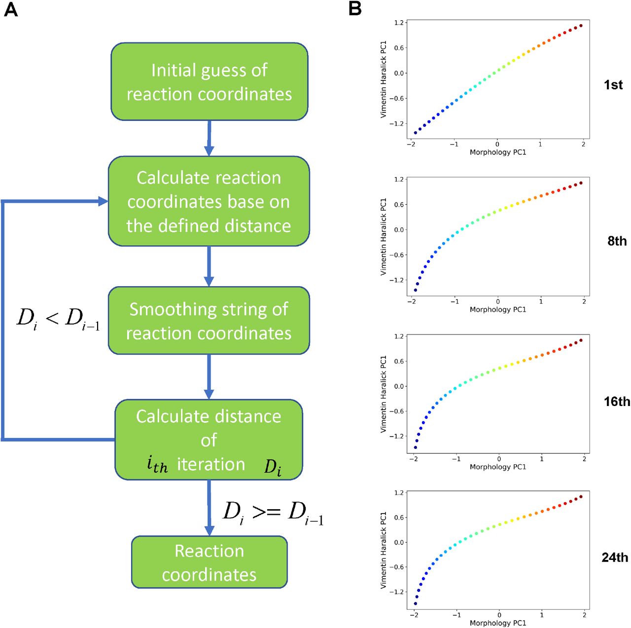
First, we set to identify the RC using a modification of the finite temperature string method6, 14, 15. The procedure starts with a trial RC to define the initial division of the Voronoi cells. One then optimizes the trial RC iteratively by minimizing the distance dispersion between the string point and sample points within each Voronoi cell. Since here we have an ensemble of continuous trajectories, we modified the iteration procedure slightly. Specifically, we minimized both the distance between the ensemble of measured reactive trajectories and the string point within each individual Voronoi cell, as well as the overall distance between each individual trajectory and the trial RC (Fig. S2, see Methods for details). The iteration procedure gives the RC of TGF-β induced EMT in A549 cells (Fig. 3A left, Fig. S3), which characterizes common features of the reactive trajectories (Fig. 3A right). Along the curve s the cell shape changes dominantly through elongation and growth (Fig. 3B top), and most of the 13 vimentin Haralick features increase or decrease monotonically and continuously over time (Fig. 3B bottom).

(A) Reconstructed RC. Left: representation of RC in the plane of morphology PC1 and vimentin Haralick PC1. Smaller cyan dots are single cell data points. Right: superimposition of the RC with four reactive trajectories (each with distinct line color) in the space of morphology PC1, vimentin Haralick PC1, and vimentin Haralick PC3. The two ends of the RC are extrapolated from epithelial and mesenchymal attractors (see Methods for details). (B) Cell shape (top) and viment Haralick feature (bottom) evolution along the RC. Haralick feature 1: Angular Second Moment; 2: Contrast; 3: Correlation; 4: Sum of Squares: Variance; 5: Inverse Difference Moment; 6: Sum Average; 7: Sum Variance; 8: Sum Entropy; 9: Entropy; 10: Difference Variance; 11: Difference Entropy; 12: Information Measure of Correlation 1; 13: Information Measure of Correlation 2. (C) Enlarged view of the red box region in Fig. 2D. The arrow associated with each data point (cyan dot) represents the value of ds/dt (white: >0, yellow: = 0, black: <0). (D) Theoretical framework of dynamics reconstruction along the RC. (E) Reconstructed dϕ/ds along the RC s (given by image point indices). (F) The RC superimposed with single cell data without TGF-β treatment (cyan dots). G) Reconstructed quasi-potentials along the RC with and without TGF-β treatment. The latter is arbitrarily shifted vertically relative to the potential with treatment. The colors of the curves in panels A, E-F, and the cell shapes in B top represent progression of EMT (starts from blue and ends in red).
For quantitative analysis, it is reasonable to assume that dynamics of the collective variables (x) can be described by a set of Langevin equations in the morphology/texture feature space, dx/ dt = F(x) + η(t), where F(x) is a governing vector field, and η are white Gaussian noises with zero mean. Then in principle one can reconstruct F(x) from the single cell trajectory data, F(x) = ⟨dx/ dt⟩. Specifically we restricted to reconstructing the dynamics along the RC, and the ansatz becomes a 1-D convection-diffusion process, ds / dt = −dϕ / ds + η. Notice that for a 1D system even without detailed balance one can define a quasi-scalar potential ϕ16, 17. Figure 3C presents an enlarged view of an area in Fig. 3A, which shows the instant velocities (ds/dt) of various trajectories segments. Numerically we related the potential gradient with the mean velocity within the i-th Voronoi cell by (Fig. 3D),

The sum was over all Ni recorded trajectory segments that locate within the i-th Voronoi cell at any time t (Fig. 3A & C). On the obtained curve of dϕ/ds v.s. s (Fig. 3E), the zeroes correspond to stationary points of the potential. We then reconstructed the quasi-potential through integrating over s,  (Fig. 3G). Also shown in Fig. 3G is the quasi-potential of the untreated cells, defined from the steady state distribution of untreated cells along the RC, ϕ0(si)∝ − log pss (si) (Fig. 3F).
The quasi-potentials in Fig. 3G provide mechanistic insights on the TGF-β induced EMT. Before TGF-β induction, cells reside on the untreated cell potential centered with a potential well corresponding to the epithelial attractor. After induction, the system relaxes following the new potential into a new well corresponding to the mesenchymal attractor. Notably in the new potential the original epithelial attractor almost disappears, reflecting that the epithelial phenotype is destablized under the applied TGF-β concentration.
One might question whether by approximating a complex dynamical process such as EMT along the 1D RC one may miss some key dynamical information. To examine such possible limitation, we adopted a different strategy of dimension reduction over the original reactive trajectories using self-organizing map (SOM). SOM is an unsupervised artificial neural network that utilize neighborhood function to represent the topology structure of input data18. The algorithm clusters the recorded cell states into 144 discrete states (Fig. 4A), and represents the EMT process as a Markovian transition process among these states (Fig. 4B). Shortest path analysis using the Dijkstra algorithm 19 over the transition matrix reveals two groups of paths: vimentin Haralick PC1 varies first, and concerted variation of morphology PC1 and vimentin Haralick PC1, with finite probabilities of transition between the two groups (Fig. 4C). This result is consistent with our previous trajectory clustering analysis using soft dynamics time warping (DTW) distance between reactive trajectories20, and suggests that indeed the 1D approximation misses some dynamical features of the process. To further support this conclusion, we also examined the density of reactive trajectories, ρR, in the plane of morphology PC1 and vimentin Haralick PC1. The contour map of ρR shows two peaks corresponding of the two groups of shorted paths in the directed network (Fig. 4D). The peak that vimentin Haralick PC1 varies firstly is higher than the peak of concerted variation, indicating more reactive trajectories along this path.

(A) Space approximation of the whole single cell data set (cyan dots) with self-organizing map into 12×12 discrete states (clusters). Red dots are centers of the clusters. (B) Directed network generated base on the self-organizing map and the transition between states. The distance between two states is defined as the negative logarithm of transition probability. (C) Shortest paths (white lines) between epithelial states (purple stars) and mesenchymal states (red stars). Green dots are the states that the shorted paths passed by. The size of a dot stands for the frequency of this dot passed by shortest paths. The width of a white line represents the frequency that these shortest paths passed by. (D) Contour map (top, superimposed with the shortest paths in panel C) and 3D surface-plot (bottom) of density of reactive trajectories in the plane of morphology PC1 and vimentin Haralick PC1. (E) RCs of the two parallel paths. (F) Cell shape (top), Haralick feature (middle), and quasi-potential evolution along RC s1. (F) Similar to E but along RC s2. The colors of the curves in panels E, F/G bottom, and the cell shapes in F/G top represent progression of EMT (starts from blue and ends in red).
To go beyond the 1D RC formalism, we grouped the reactive trajectories based on the DTW distance, then identified the RCs for each group separately following the modified string method (Fig. 4E). The two RCs first diverge from the E region to follow two distinct paths, then converge within the M region. In one group (Fig. 4F), most of the Haralick feature changes take place before major morphology change. The two segments of the quasi-potential curve with shallow and steep slopes also reflect the two-stage dynamics. For the group with concerted dynamics (Fig. 4G), both cell shape and Haralick features vary gradually along the RC. The quasi-potential also decreases steadily, only interrupted by a short transition region. These analyses provide direct evidence that TGF-β induced EMT proceeds through parallel paths with distinct dynamical features.
DISCUSSIONS
In summary, through analyzing experimentally measured single cell trajectories with dynamical systems theories we obtained quantitative mechanistic insights of TGF-β induced EMT. The dynamics can be mapped to that of a chemical system transiting from the ground to an excited potential then relaxing to a new stable state. This work demonstrates the existence of a unified theoretical framework describing transition and relaxation dynamics in systems with and without detailed balance. CPTs, with relevant spatial and temporal scales orders of magnitude larger than typical molecular systems and thus more accessible for multiplex quantitative measurements, can serve as an ideal test ground for reaction rate theories.
AUTHOR CONTRIBUTIONS
J. X. designed the research; W. W. and J. X. performed the research and wrote the paper.
SUPPLEMENTAL FIGURE CAPTION

(A) Representation in the Morphology PC1-Vimentin Haralick PC1 space. (B) Representation in the Vimentin Haralick PC3-Vimentin Haralick PC4 space.

(A) Flow chart of the procedure. (B) Example RC curves obtained at different iteration cycle.

The RC is shown in the Vimentin Haralick PC3-Vimentin Haralick PC4 spacesuperimposed with data points (cyan dots) under TGF-β treatment (A) and under control condition (B), respectively.
METHODS
1) Procedure for determining a reaction coordinate
We followed a procedure adapted from what used in the finite temperature string method for numerical searching of reaction coordinate and non-equilibrium umbrella sampling14, 15, with a major difference that we used experimentally measured single cell trajectories (Fig. S2).
Identify the starting and ending points of the reaction path as the means of data points in the epithelial and mesenchymal regions, respectively. The two points are fixed in the remaining iterations.
Construct an initial guess of the reaction path that connects the two ending points in the feature space through linear interpolation. Discretize the path with N (= 35) points (called images, and the k-th image denoted as sk with corresponding coordinate X(sk)) uniformly spaced in arc length.
Collect all the reactive single cell trajectories that start from the epithelial region and end in the mesenchymal region.
Divide the multi-dimensional state space by a set of Voronoi polyhedra containing individual images. Associate each point of measured single cell trajectories, denoted as
 for the point on trajectory u at time tα, to a polyhedron containing the image closest to the point. Define the distance between image sk and a given single cell reactive trajectory, dk,u, as the distance between each image on the path to the closest point on the trajectory, . Then the reaction coordinate is the path (image set) that minimizes the following score function, , where w is a parameter that specifies the relative weights between the two terms in the right hand of the expression, and we used w = 30 in our calculations. We carried out the minimization procedure through an iterative process. For a given trial path defined by the set of image points, we calculated a set of average points using the following equations,. Next we updated the continuous reaction path through cubic spline interpolation of the average positions21, and generated a new set of N images {X(sk)} that are uniformly distributed along the new reaction path. We set a smooth factor, i.e., the upper limit of , as 0.05 for calculating the RC in Fig. 3, and 0.1 for the paths in Fig. 4. We used a larger smooth factor for the latter to avoid overfitting as there is less data in each of the two groups compared to the overall data set used in Fig. 3.
We iterated the whole process in step 3 until there was no further change of Voronoi polyhedron assignments of the data points.
For obtaining the quasi-potential of a larger range of s, extrapolate the obtained reaction path forward and backward by adding additional image points (5 for the single reaction path and 2 for the two parallel reaction paths) beyond the two ends of the path linearly, respectively. These new image points are also uniformly distributed along s as the old image sets do. Re-index the whole set of image points as {s0, s1,…, si ,…, sN ,sN+1}.


2) Reconstruction of quasi-potential along the reaction coordinate
Based on the theoretical framework in Fig. 3D, we followed the procedure below:
The N + 2 image points of an identified RC divide the space in N + 2 Voronoi cells that data points can assign to. Ignore the first and last Voronoi cells, and use the remaining N cells for the remaining analyses.
Within the i-th Voronoi cell, calculate the mean drift speed (and thus dϕ / ds) at si approximately by
where s(X) is the assumed value along s for a cell state X in the morphology/texture feature space. The sum is over all time and all data points from all the recorded trajectories that lie within the i-th Voronoi cell (s(X(t)) = si), and ∆t =1 is one recording time interval. Using data points from all instead of just reactive trajectories is necessary for unbiased sampling within each Voronoi cell withCalculate the quasi-potential through numerical integration,
. The exact value of ϕ(s0) does not affect the quasi-potential shape.


3) calculation of dynamics of morphology and Haralick features along reaction path
The reaction path is calculated in the principal component (PC) space of morphology PC1, vimentin Haralick PC1, PC3 and PC4. Distribution of cells show significant shift before and after TGF-β treatment in these dimensions7. To reconstruct dynamics in the original features space from PCs, the reaction path’s coordinates on the other dimensions of PC are set as means of data in the corresponding Voronoi cell of each point on the reaction path. We obtain the reaction path in full dimension of PC space. The dynamics of morphology and Haralick features are calculated by inverse-transform of coordinates of PCs.
4) Self-organizing map and shortest transition paths in the directed network
The self-organizing map is an unsupervised machine learning method to represent the topology structure of date sets. We used a 12×12 grid (neurons) to perform space approximation of all reactive trajectories (Fig. 4A). The SOM was trained for 50 epochs on the data with Neupy (http://neupy.com/pages/home.html). We set the learning radius as 1 and standard deviation 1. These neurons divide the data into 144 micro-clusters ({ψ}). With the single cell trajectory data, we counted the transition probabilities from cluster i to cluster j (including self), with  .If the transition probability is smaller than 0.01, the value is then reset as 0. With the transition probability matrix, we built a directed network of these 144 neurons (Fig. 4B). The distance (weight) of the edge between neuron ψi and neuron ψj is defined as the negative logarithm of transition probability (− log pi,j). We ignored the connection between two clusters. We set the neurons that close to the center of epithelial and mesenchymal state (sphere with radius = 0.7) as epithelial community and mesenchymal community, respectively, and used Dijkstra algorithm to find the shortest path between each pair of epithelial and mesenchymal neurons19 with NetworkX22. We recorded the frequency of neurons and edge between these neurons that are past by these shortest paths.
5) Calculation of density of reactive trajectory
The density of reactive trajectory on the plane of morphology PC1 and vimentin Haralick PC1 is calculated with the following procedure:
Divide the whole plane into 200×200 grids.
In each grid, count the number of reactive trajectory (only the parts of each reactive trajectory that are in the intermediate region are taken into consideration) that enters and leaves it. If a reactive trajectory passes certain grid multiple times, only 1 is added in this grid’s density. Thus, the density matrix is obtained.
Use Gaussian filter to smooth the obtained density matrix. The standard deviation is 2 and the truncation is 2 (truncate at twice of the standard deviation).
6) Reconstruction of quasi-potential along parallel paths
We used tslearn to calculate the DTW distance between two reactive trajectories, then performed K-Means clustering23 on the DTW distance matrix7, 20 to cluster the reactive trajectories into two groups. We set DTW γ (parameter of the kernel in the algorithm) as 50. We then followed the procedure in Methods (1) to reconstruct the RC for each group. We reconstructed the quasi-potentials using all trajectories. For a trajectory not belonging to the reactive trajectory ensemble, we assigned it to one of the two group associated to the two RCs, {s1} = {s1,1,…, s1,i, …, s1,N} and {s2} = {s2,1,…, s2,i, …, s2,N} as follows. We first assigned data points of this trajectory to the Voronoi cells of {s1} and {s2}, respectively, and identified its maximum coordinates s1,m and s2,m on the RCs. We then calculated the DTW distances between this non-reactive trajectory and {s1,1,…, s1,i, …, s1,m} , and {s2,1,…, s2,i ,…, s2,m} , respectively. This trajectory was grouped into the reaction path that has smaller DTW distance with it. After grouping all the trajectories, we calculated the drift speed ⟨ds / dt⟩ and quasi-potential ϕ(s) of each path using their corresponding trajectories, following the definition and procedure described in Methods (2).
ACKNOWLEDGMENTS
This work was partially supported by the National Science Foundation [DMS-1462049], National Cancer Institute [R01CA232209], National Institute of Diabetes and Digestive and Kidney Diseases (R01DK119232) to JX.
Reference


