

Abstract
The massive growth of single-cell RNA-sequencing (scRNAseq) and methods for its analysis still lacks sufficient and up-to-date benchmarks that would guide analytical choices. Moreover, current studies are often focused on isolated steps of the process. Here, we present a flexible R framework for pipeline comparison with multi-level evaluation metrics and apply it to the benchmark of scRNAseq analysis pipelines using datasets with known cell identities. We evaluate common steps of such analyses, including filtering, doublet detection (suggesting a new R package, scDblFinder), normalization, feature selection, denoising, dimensionality reduction and clustering. On the basis of these analyses, we make a number of concrete recommendations about analysis choices. The evaluation framework, pipeComp, has been implemented so as to easily integrate any other step or tool, allowing extensible benchmarks and easy application to other fields (https://github.com/plger/pipeComp).
Background
Single-cell RNA-sequencing (scRNAseq) and the set of attached analysis methods are evolving fast, with more than 560 software tools available to the community [1], roughly half of which are dedicated to tasks related to data processing such as clustering, ordering, dimension reduction or normalization. This increase in the number of available tools follows the development of new sequencing technologies and the growing number of reported cells, genes and cell populations [2]. As data processing is a critical step in any scRNAseq analysis, affecting downstream analysis and interpretation, it is critical to evaluate the available tools.
A number of good comparison and benchmark studies have already been performed on various steps related to scRNAseq analysis and can guide the choice of methodology [3,4,5,6,7,8,9,10,11,12,13,14,15,16,17,18]. However these recommendations need constant updating and often leave open many details of an analysis. Another missing aspect of current benchmarking studies is their limitation to capture all aspects of scRNAseq processing workflow. Although previous benchmarks already brought valuable recommendations for data processing, some only focused on one aspect of data processing (e.g., [11]), did not evaluate how the tool selection affects downstream analysis (e.g., [14]) or did not tackle all aspects of data processing, such as doublet identification or cell filtering (e.g., [15]). A thorough evaluation of the tools covering all major processing steps is however urgently needed as previous benchmarking studies highlighted that a combination of tools can have a drastic impact on downstream analysis, such as differential expression analysis and cell-type deconvolution[15,3]. It is then critical to evaluate not only the single effect of a preprocessing method but also its positive or negative interaction with all parts of a workflow.
Here, we develop a flexible R framework for pipeline comparison and evaluate the various steps of analysis leading from an initial count matrix to a cluster assignment, which are critical in a wide range of applications. We collected real datasets of known cell composition (Table 1) and used a variety of evaluation metrics to investigate in a multilevel fashion the impact of various parameters and variations around a core scRNAseq pipeline. Although we use some datasets based on other protocols, our focus is especially on droplet-based datasets that do not include exogenous control RNA (i.e. spike-ins); see Table 1 and Figure 1 for more details. In addition to previously-used benchmark datasets with true cell labels [6,12], we simulated two datasets with a hierarchical subpopulation structure based on real 10x human and mouse data using muscat [19]. Since graph-based clustering [20] was previously shown to consistently perform well across several datasets [6,12], we used the Seurat pipeline as the starting point to perform an integrated investigation of: 1) doublet identification, 2) cell filtering, 3) normalization, 4) feature selection, 5) dimension reduction, 6) clustering. We compared competing approaches and also explored more fine-grained parameters and variations on common methods. Importantly, the success of methods at a certain analytical step might be dependent on choices at other steps. Therefore, instead of evaluating each step in isolation, we developed a general framework for evaluating nested variations on a pipeline and suggest a multilevel panel of metrics. Finally, we evaluate several recent methods and provide concrete recommendations.

Results
A flexible framework for pipeline evaluation
The pipeComp package defines a pipeline as, minimally, a list of functions executed consecutively on the output of the previous one (Figure 2A). In addition, optional benchmark functions can be set for each step to provide standardized, multi-layered evaluation metrics. Given such a PipelineDefinition object, a set of alternative parameters (which might include different subroutines) and benchmark datasets, the runPipeline function then proceeds through all combinations of arguments, avoiding recomputing the same step twice and compiling evaluations (including running time) on the fly. Variations in a given parameter can be evaluated using all metrics from this point downward in the pipeline. This is especially important because end-point metrics, such as the adjusted Rand index (ARI) [21] for clustering, are not perfect. For example, although the meaning of an ARI score is independent of the number of true subpopulations [22], the number of clusters called is by far the most important determinant of the score: the farther it is from the actual number of subpopulations, the worse the ARI (Supplementary Figure 17). In this context, one strategy has been to cluster across various resolutions and only consider the results that have the right number of clusters [6]. While this has the virtue of making the results comparable, in practice the number of subpopulations is typically unknown and tools that operate well in this optimal context might not necessarily be best overall. Clustering results are also very sensitive and might not always capture improvements in earlier steps of the pipeline. We therefore favour monitoring several complementary metrics across multiple steps of the process.

A: The package is built around a PipelineDefinition S4 class which defines a set of functions to be executed consecutively, as well as optional evaluation functions for each step. Each step can accept of number of parameters whose alternative values are provided as a list. All (or subsets of) combinations of parameters can then be simultaneously ran and evaluated using the runPipeline function. B: Scheme representing the application of pipeComp to evaluate a range of methods that are commonly used in scRNAseq studies and some of the metrics monitored at various steps.
A clustering output is relatively fragile to variations in the pipeline. We therefore wanted to capture whether the effect of a given parameter alteration is robust to changes in the rest of the pipeline, or rather specific to a set of other pipeline parameters. We proceeded in a step-wise fashion, first testing a large variety of parameters at the early steps of the pipeline along with only a set of mainstream options downstream, then selecting main alternatives and proceeding to a more detailed benchmark of the next step (Figure 2B).
Filtering
Doublet detection
Doublets, defined as two cells sequenced under the same cellular barcode (e.g., being captured in the same droplet), are fairly frequent in scRNAseq datasets, with estimates ranging from 1 to 10% depending on the platform and cell concentration used [23,24]. While doublets of the same cell type are relatively innocuous for most downstream applications due to their conservation of the relative expression between genes, doublets formed from different cell types or states are likely to be misclassified and could potentially distort downstream analysis. In some cases, doublets can be identified through their unusually high number of reads and detected features, but this is not always the case (Supplementary Figure 2). A number of methods were developed to identify doublets, in most cases by comparing each cell to artificially-created doublets [25,26,27]. We first evaluated the capacity of these methods to detect doublets using the two 10x datasets with cells of different genetic identity [12], using SNP genotypes as the ground truth. For the sole purpose of this section, we included an additional dataset with SNP information but lacking true cell labels [24]. Of note, SNP-based analyses also call doublets created by cells of the same cell type (but from different individuals) and which are generally described as homotypic (as opposed to neotypic or heterotypic doublets, i.e. doublets from different cell types). These homotypic doublets might not be identifiable from the mere gene counts, and their identification is not generally the primary aim of doublet callers since they are often considered innocuous and, when across individuals, can be identified through other means (e.g., SNPs). We therefore do not expect a perfect accuracy in datasets involving cells of the same type across individuals (as in the demuxlet dataset).
We tested DoubletFinder [25] and scran’s doubletCells [26], both of which use similarity to artificial doublets, and scds [27], which relies on a combination of co-expression and binary classification. DoubletFinder integrates a thresholding based on the proportion of expected doublets, while scran and scds return scores that must be manually thresholded. In these cases, we ensured that the right number of cells would be called doublets. In addition to these methods, we reasoned that an approach such as DoubletFinder could be simplified by being applied directly on counts and by using a pre-clustering to create neotypic/heterotypic doublets more efficiently. We therefore developed a simple and fast Bioconductor package implementing this method for doublet detection, scDblFinder, with the added advantage of accounting for uncertainty in the expected doublet rate and using meta-cells from the clusters to even include triplets (see Methods).
While most methods accurately identified the doublets in the 3 cell lines dataset (mixology10×3cl), the other two datasets proved more difficult (Figure 3A). scDblFinder achieved comparable or better accuracy than top alternatives while being the fastest method (Figure 3B). Across datasets, cells called as doublets tended to be classified in the wrong cluster more often than other cells (Figure 3C). We also found that scDblFinder improved the accuracy of the clustering across all benchmark datasets even when, by design, the data contained no heterotypic doublet (Figure 4).
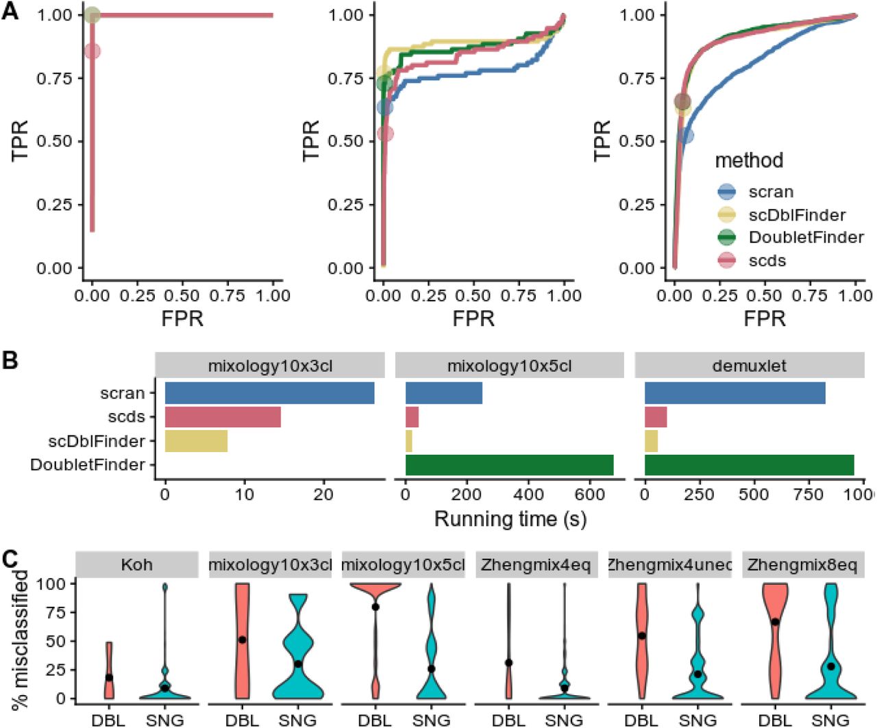
A: Receiver operating characteristic (ROC) curves of the tested doublet detection methods for three datasets with SNP-identified doublets. Dots indicate threshold determined by the true number of doublets. B: Running time of the different methods (DoubletFinder failed on one of the datasets). C: Rate of misclassification of the cells identified by scDblFinder as doublets (DBL) or singlets (SNG), across a large range of clustering analysis. Even in datasets which should not have neotypic doublets, the cells identified as such tend to be misclassified.

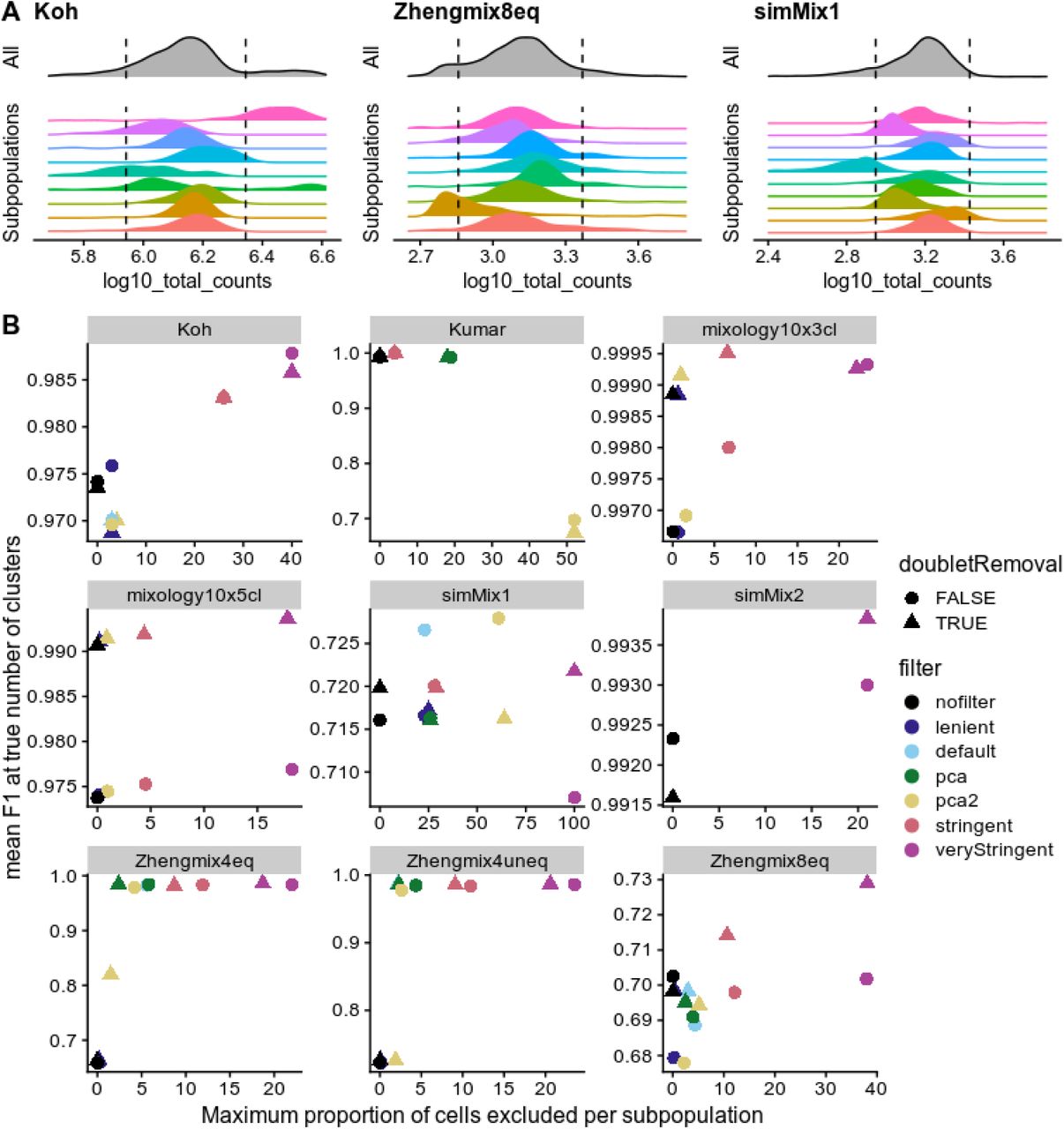
A: Filtering on the basis of distance to the whole distribution can lead to strong bias against certain subpopulations. The dashed line indicates a threshold of 2.5 median absolute deviations (MADs) from the median of the overall population. B: Relationship between the maximum subpopulation exclusion rate and the average clustering accuracy per subpopulation across various filtering strategies. Of note, doublet removal appears to be desirable even when, due to the design, there are no heterotypic doublets in the data. The PCA methods refer to multivariate outlier detected as implemented in scater (see Methods for details).
Excluding more cells is not necessarily better
Beyond doublets, a dataset might include low-quality cells whose elimination would reduce noise. This has for instance been demonstrated for droplets containing a high content of mitochondrial reads, often as a result of cell degradation and resulting loss of cytoplasmic mRNAs [28]. A common practice is to exclude cells that differ considerably from most other cells on the basis of such properties. This can for instance be performed through the isOutlier function from scater that measures, for a given control property, the number of median absolute deviations (MADs) of each cell from the median of all cells. Supplementary Figure 1 shows the distributions of some of the typical cell properties commonly used. Of note, these properties tend to be correlated, with some exceptions. For example, while a high proportion of mitochondrial reads is often correlated with a high proportion of the counts in the top features, there can also be other reasons for an over-representation of highly-expressed features (Supplementary Figure 3), such as an over-amplification in non-UMI datasets. In our experience, 10X datasets also exhibit a very strong correlation between the total counts and the total features even across very different cell types (Supplementary Figure 4). We therefore also measure the ratio between the two and treat cells strongly departing from this trend with suspicion.
Reasoning that the cells we wish to exclude are the cells that would be misclassified, we measured the rate of misclassification of each cell in each dataset across a variety of clustering pipelines, correcting for the median misclassification rate of the subpopulation and then evaluated what properties could be predictive of misclassification (Supplementary Figures 5-7). We could not identify any property or simple combination thereof that would be consistently predictive of misclassification; the only feature that consistently stood out across multiple datasets (the Zheng datasets) was that cells with very high read counts have a higher chance of being misclassified.
We next investigated the impact of filtering according to various criteria (see Methods). An important risk of excluding cells on the basis of their distance from the whole distribution of cells on some properties (e.g., library size) is that these properties tend to have different distributions across subpopulations. As a result, thresholds in terms of number of MADs from the whole distribution can lead to strong biases against certain subpopulations (Figure 4A). We therefore examined the tradeoff between the increased accuracy of filtering and the maximum proportion of cells excluded per subpopulation (Figure 4B and Supplementary Figure 8). Since filtering changes the relative abundance of the different subpopulations, global clustering accuracy metrics such as ARI are not appropriate here. We therefore calculated the per-subpopulation precision and recall using the Hungarian algorithm [29] and monitored their mean F1 score. A first observation was that, although the stringent filtering tended to be associated with an increase in accuracy, it could also become deleterious and most of the benefits could be achieved without very stringent filtering and minimizing subpopulation bias (Figure 4B). Applying the same filtering criteria on individual clusters of cells (identified through scran’s quickCluster method) resulted in nearly no cell being filtered out. This suggests that filtering on the global population tends to discard cells of subpopulations with more extreme properties (e.g. high library size), rather than low-quality cells. Finally, by changing the distributions, the doublet removal step in conjunction with filtering sometimes resulted in a net decrease in the proportion of excluded cells while retaining or improving accuracy. We therefore recommend the use of doublet removal followed by relatively mild filtering, such as is implemented in our ‘default’ filtering (see Methods).
Filtering features by type
Mitochondrial reads have been associated with cell degradation and there is evidence that ribosomal genes can influence the clustering output, hiding other biological structure in the analysis [7]. We therefore investigated whether excluding one category of features or the other, or using only protein-coding genes, had an impact on the ability to distinguish subpopulations (Supplementary Figure 9). Removal of ribosomal genes robustly reduced the quality of the clustering, suggesting that they represent real biological differences between subpopulations. Removing mitochondrial genes and restricting to protein-coding genes had a very mild impact.
Normalization and scaling
We next investigated the impact of different normalization strategies. Beside the standard log-normalization included in Seurat, we tested scran’s pooling-based normalization [30], sctransform’s variance-stabilizing transformation [31], and normalization based on stable genes [32,33]. In addition to log-normalization, the standard Seurat clustering pipeline performs per-feature unit-variance scaling so that the PCA is not too strongly dominated by highly-expressed features. We therefore included versions of the different normalization procedures, with or without a subsequent scaling (sctransform’s variance-stabilizing transformation involves an approach analogous to scaling). Seurat’s scaling function also includes the option to regress out the effect of certain covariates. We tested its performance by using the proportion of mitochondrial counts and the number of detected features as covariates. Finally, it has been proposed that the use of stable genes, in particular cytosolic ribosomal genes, can be used to normalize scRNAseq[33]. We therefore evaluated a simple linear normalization based on the sum of these genes, as well as nuclear genes.
An important motivation for the development of sctransform was the observation that, even after normalization, the first principal components of various datasets tended to correlate with library size, suggesting an inadequate normalization [31]. However, as library size tends to vary across subpopulations, part of this effect can simply reflect biological differences. We therefore assessed to what extent the first principal component still retained a correlation with the library size and the number of detected features, removing the confounding covariation with the subpopulations (Figure 5A). The simple step of scaling tended to remove much of the correlation with these features and, in the absence of scaling, standard Seurat normalization resulted in fairly high correlation with technical covariates. sctransform led to the lowest correlation but most methods, including normalization based on stable genes, were able to remove most of the correlation when combined with scaling. The only exception is Seurat normalization with scaling regressing out covariates, which surprisingly increased the correlation in 8 of the 9 datasets.

‘Seurat.feat_mt_regress’ regresses out the number of features and proportion of mitochondrial reads during scaling; ‘Seurat.feat_regress’ regresses out the number of features only. Residual correlation of the first principal component with library size (left) and detection rate (right), after accounting for biological differences between subpopulations. B: Average silhouette width per true subpopulation, where higher silhouette width means a higher separability. C: Clustering accuracy (Seurat clustering), measured by the ARI at the true number of cluster (left) and by the average mutual information (MI) of the cluster assignment with true subpopulations.
We further evaluated normalization methods by investigating their impact on the separability of the subpopulations (Figure 5B-C). Since clustering accuracy metrics such as the ARI are very strongly influenced by the number of clusters, we complemented it with silhouette width [34] and mutual information. We found most methods (including no normalization at all) to perform fairly well in most of the subpopulations. Scaling tended to reduce the average silhouette width of some subpopulations and to increase that of some less distinguishable ones and was generally, but not always, beneficial on the accuracy of the final clustering. Regressing out covariates systematically gave poorer performance on all metrics. sctransform systematically outperformed other methods and, even though it was developed to be applied to data with unique molecular identifiers (UMI), it also performed fairly well with the Smart-seq protocol (Koh and Kumar datasets).
Finally, we monitored whether, under the same downstream clustering analysis, different normalization methods tended to lead to an over- or under-estimation of the number of clusters. Although some methods had a tendency to lead to a higher (e.g., sctransform) or lower (e.g., stable genes) number of clusters, the effect was very mild and not entirely systematic (Supplementary Figure 10).
Feature selection
A standard clustering pipeline typically involves a step of highly-variable genes selection, which is complicated by the digital nature and the mean-variance relationship of (sc)RNAseq. Seurat’s earlier approaches involved the use of dispersion estimates standardized for the mean expression levels, while more recent versions (≥3.0) rely on a different measure of variance, again standardized. While adjusting for the mean-variance relationship removes much of the bias towards highly-expressed genes, it is plausible that this relationship may in fact sometimes reflects biological relevance and would be helpful in classifying cell types. Another common practice in feature selection is to use those with the highest mean expression. Recently, [35] instead suggested to use deviance, while sctransform provides its own ordering of genes based on transformed variance.
Reasoning that a selection method should ideally select genes whose variability is higher between subpopulations than within, we first assessed to what extent each method selected genes with a high proportion of variance or deviance explained by (real) subpopulation. As the proportion of variability in a gene attributable to subpopulations can be measured in various ways, we first compared three approaches: ANOVA on log-normalized count, ANOVA on sctransform normalization, and deviance explained. The ANOVAs performed on a standard Seurat normalization and on sctransform data were highly correlated (Supplementary Figure 11A). These estimates were also in good agreement with the deviance explained, although lowly-expressed genes could have a high deviance explained without having much of their variance explained by subpopulation (Supplementary Figure 11B-D). We therefore compared the proportion of the cumulative variance/deviance explained by the top X genes that could be retrieved by each gene ranking method (Supplementary Figures 12-13). We first focused on the first 1000 genes to highlight the differences between methods, although a higher number of selected genes decreased the differences between methods (Supplementary Figures 12-14). The standardized measures of variability were systematically worse than their non-standardized counterparts in selecting genes with a high proportion of variance explained by subpopulation. Regarding the percentage of deviance explained however, the standardized measures were often superior (Figure 6A and Supplementary Figures 12-13). Deviance proved the method of choice to prioritize genes with a high variance explained by subpopulations (with mere expression level proving surprisingly good) but did not perform so well to select genes with a high deviance explained.

A: Ability of different feature ranking methods to capture genes with a high proportion of variance (left) or deviance (right) explained by real subpopulations. The asterix denotes the default Seurat method. B: Accuracy of clusterings (at the true number of clusters) when selecting 1000 genes using the given methods. Based on standard Seurat normalization (left) or sctransform (right). The vst.varExp and devianceExplained methods correspond to the estimates used in A to evaluate the selection methods and were included here only for validation purpose.
We next evaluated how the use of different feature selection methods affected the clustering accuracy (Figure 6B). To validate the previous assay on the proportion of variance/deviance explained by real populations, we included genes that maximized these two latter measures. Interestingly, while these selections were on average the top-ranking methods, they were not systematically best for all datasets. The previous observations were reflected in the ARI of the resulting clustering (Figure 6B): non-standardized measures of variability, including mere expression level, tended to outperform more complex metrics. In general, we found deviance and unstandardized estimates of variance to provide the best results across datasets and normalization methods. Increasing the number of features selected also systematically led to an increase in the accuracy of the clustering, typically plateauing after 4000 features (Supplementary Figure 14).
Dimensionality reduction
Since the various PCA approaches and implementations were recently benchmarked in a similar context [14], we focused on widely used approaches which had not yet been compared: Seurat’s PCA, scran’s denoisePCA, and GLM-PCA [35]. When relevant, we combined them with sctransform normalization. Given that Seurat’s default PCA weights the cell embeddings by the variance of each component, we also evaluated the impact of this weighting with each method.
The impact of the choice of dimensionality reduction method was far greater than that of normalization or feature selection (e.g., Supplementary Figure 15). GLM-PCA tended to increase the average silhouette width of already well-defined subpopulations, but Seurat’s PCA procedure however proved superior on all metrics (Figure 7). Overall, weighting the principal components by their variance (as Seurat does) had a positive impact on silhouette widths and ARI scores.

A: Average silhouette width per subpopulation resulting from combinations of normalization and dimension reductions. B: Clustering accuracy, mean proportion of the variance in the first 5 components explained by real subpopulations (center), and median ARI of the resulting clustering (right).
Estimating the number of dimensions
A common step following dimension reduction is the selection of an appropriate number of dimensions to use for downstream analysis. Since Euclidean distance decreases as the number of non-discriminating dimensions increases, there is usually a trade-off between selecting enough dimensions to keep most information and excluding smaller dimensions that may represent technical noise or other unwanted sources of variation. Overall, increasing the number of dimensions robustly led to a decrease in the number of clusters (Supplementary Figures 10 and 15). This tended to affect the accuracy of the clustering (Supplementary Figure 16), although in both cases (number of clusters and ARI) Seurat’s resolution parameter had a much stronger impact.
Different approaches have been proposed to select the appropriate number of dimensions, from the visual identification of an ‘Elbow’ (inflexion point) of the variance explained, to more complex algorithms. We evaluated the performance of dimensionality estimators implemented in the intrinsicDimension package [36], as well as common procedures such as the ‘elbow’ method (inflexion point in the variance explained by each component), some scRNAseq-specific methods such as the JackStraw procedure [37] or scran’s denoisePCA [26], and the recent application of Fisher Separability analysis [38].
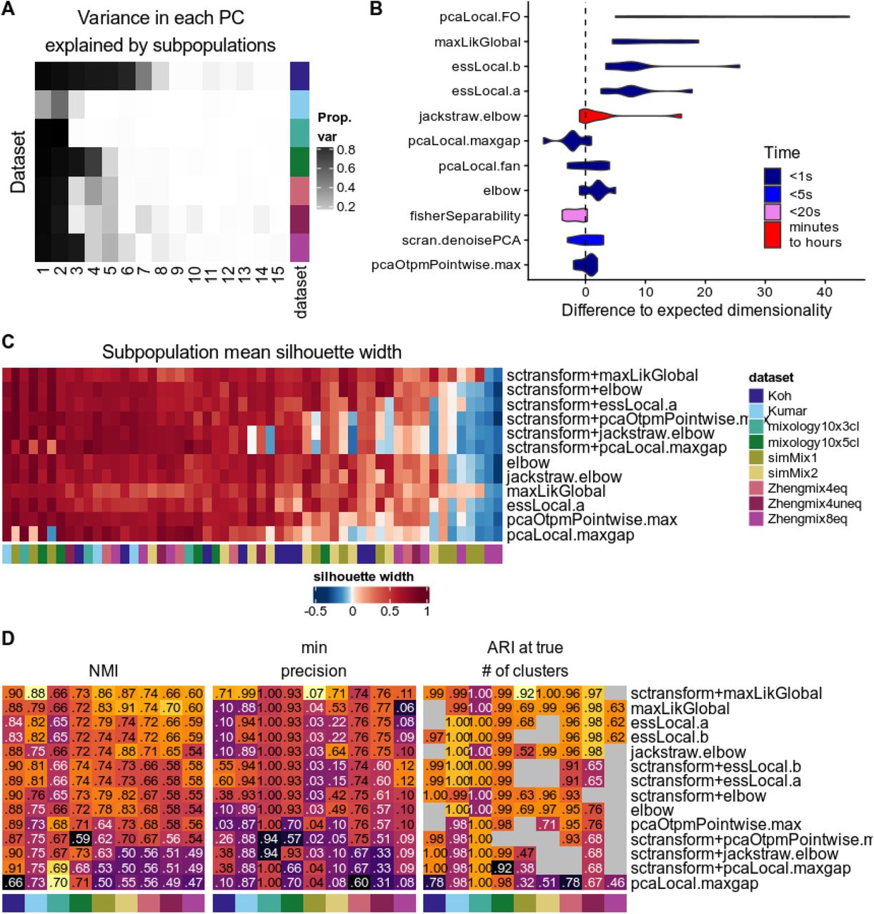
We compared the various estimates of dimensionality in their ability to retrieve the intrinsic number of dimensions in a dataset, based on Seurat’s weighted PCA space. As a first approximation of the true dimensionality, we computed the variance in each principal component that was explained by the subpopulations, which sharply decreased after the first few components in most datasets (Figure 8A). Figure 8B shows the difference between the dimension estimates of the above methods and that based on the subpopulations (i.e. from Figure 8A). Of note, the methods differ widely in view of their computing time (Figure 8B) and we saw no relationship between the accuracy of the estimates and the complexity of the method. Reasoning that over-estimating the number of dimensions is less problematic than under-estimating it, we kept the former methods for a full analysis of their impact on clustering (Figure 8C-D), when combined with sctransform or the standard Seurat normalization. Although most methods performed well on the various clustering measures, the global maximum likelihood based on translated Poisson Mixture Model (maxLik-Global) provided the dimensionality estimate that best separated the subpopulations (Figure 8C) and resulted in the best clustering accuracy (Figure 8D). This method systematically selected many more components than were associated with the subpopulations, suggesting that although these additional components appear individually uninformative, in combination they nevertheless contribute to classification.

A: Estimated dimensionality using the proportion of variance in each component explained by the true subpopulations. B: Difference between ‘real’ dimensionality (from A) and dimensionality estimation methods, along with computing time. C: Average silhouette width per subpopulation across a selection of methods, combined with sctransform or standard Seurat normalization. D: Clustering accuracy across the normalization/dimensionality estimation methods.
Clustering
The last step evaluated in our pipeline was clustering. Given previous works on the topic [6,7] and the success of graph-based clustering methods for scRNAseq, we restricted our evaluation to Seurat’s method and two scran SNN-based clustering approaches, based on random walks (walktrap method) or on the optimization of the modularity score (fast_greedy). Again, the tested methods were combined with Seurat’s standard normalization and sctransform, otherwise using the parameters found optimal in the previous steps.
Since ARI is dominated by differences in the number of clusters (Supplementary Figure 17) and no single metric is perfect, we diversified them (Figure 9). Mutual information (MI) has the virtue of not decreasing when a true subpopulation is split into two clusters, which is arguably less problematic (and might well reflect unknown biological subgroups), but as a consequence it can be biased towards methods producing higher resolution clustering. Similarly, precision per true subpopulation is considerably more robust to differences in the number of clusters. We also tracked the mean F1 score and the ARI at the true number of clusters.

Clustering accuracy of common clustering tools in combination with sctransform and standard Seurat’s normalization.
The MI score and minimum precision, which are largely independent of the estimated number of clusters, were overall higher for the walktrap method (Figure 9), while the mean F1 score favored both scran methods (walktrap and fast greedy) over Seurat. Finally, the ARI score at the true number of clusters, when available, showed similar performances. However, because Seurat’s resolution parameter had a large impact on the number of clusters identified (Supplementary Figure 18), Seurat could always be coerced into producing the right number of clusters. Instead, the number of clusters found by scran was considerably less influenced by the available parameters (number of nearest neighbors or steps in the random walk - see Supplementary Figure 18), and as a result scran-based clustering sometimes never produced a partitioning with the right number of clusters. This observation, along with scran’s higher MI score, suggest that scran sometimes simply divides a real subpopulation into two clusters (possibly tracking some unknown biological differences) rather than committing misclassification errors. Overall, the walktrap method appeared superior to the fast greedy algorithm and was generally less prone to misclassification than Seurat clustering, although the latter offered more control over the resolution. Finally, some poorly distinguishable subpopulations from both the Zhengmix8eq and simMix1 datasets remained very inaccurately classified by all methods and in regards to all metrics.
Further extensions to the pipeline: imputation/denoising
The basic pipeline presented here can be extended with additional analysis steps while keeping the same evaluation metrics. To demonstrate this, we evaluated various imputation or denoising techniques based on their impact on classification. Since preliminary analysis showed that all methods performed equally well or better on normalized data, we applied them after filtering and normalization, but before scaling and reduction. Although some of the methods (e.g., DRImpute_process and alra_norm) did improve the separability of some more elusive subpopulations, no method had a systematically positive impact on the average silhouette width across all subpopulations (Figure 10A). When restricting ourselves to clustering analyses that yielded the ‘right’ number of clusters, all tested methods improved classification compared to a scenario with no imputation step (‘none’ label, Figure 10B). However, the situation was not so straightforward with alternative metrics, where some methods (e.g., enhance) consistently underperformed. 10X datasets, which are typically characterized by a lower per-cell coverage and feature detection rate, benefited more from imputation and, in this context, DrImpute and dca tended to show the best performance. On the contrary, imputing on normalized counts originating from Smart-seq technology was instead rather deleterious to the clustering accuracy.
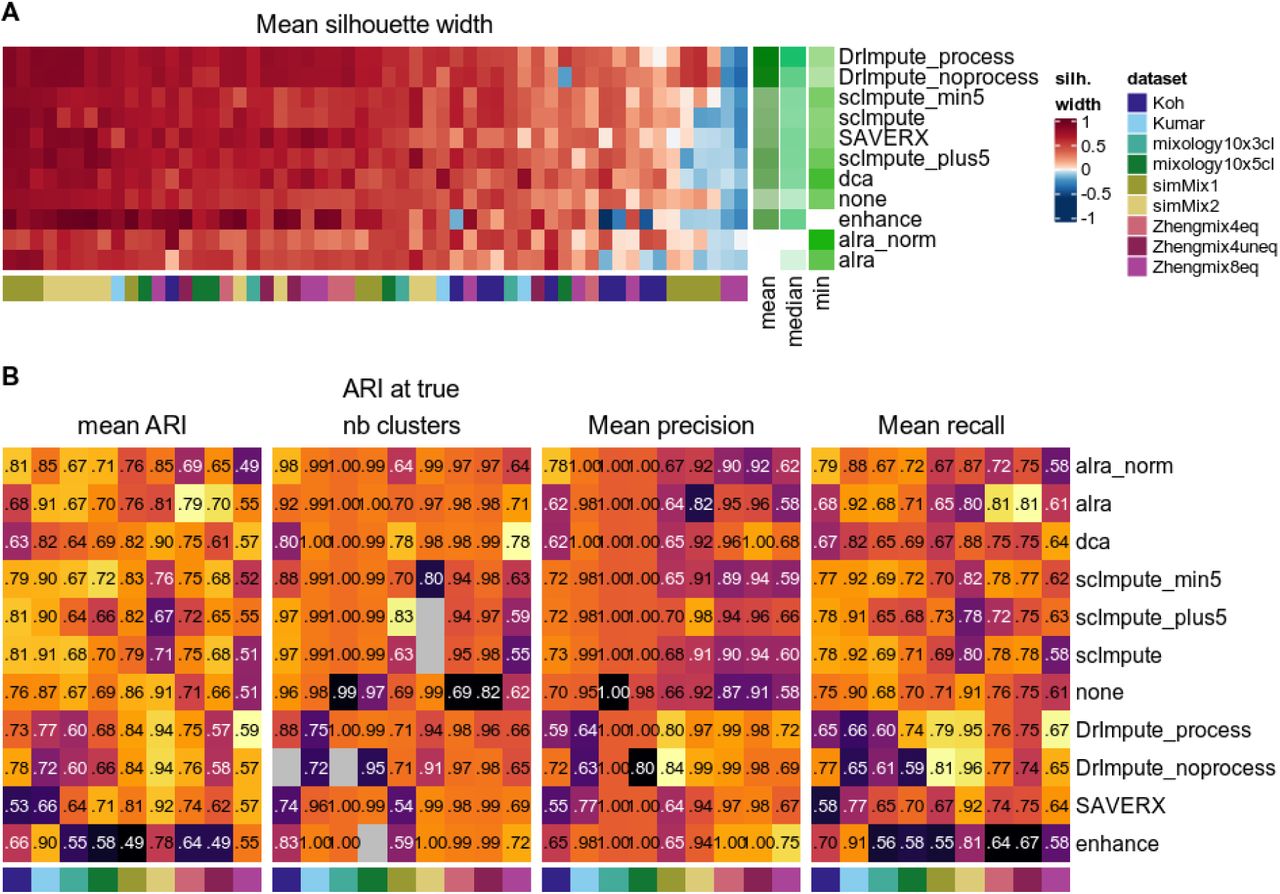
Average silhouette width per subpopulation (A) and clustering accuracy (B) with or without (indicated as none) application of a denoising/imputation method.
Discussion
Concrete recommendations
On the basis of our findings, we can make a number of concrete analysis recommendations, also summarized in Figure 11:
Filtering
Doublet detection and removal is advised and can be performed at little computing cost with software such as scDblFinder or scds.
Distribution-based cell filtering fails to capture doublets and should use relatively lenient cutoffs (e.g., 5 MADs, or 3 MADs in at least 2 distributions) to exclude poor-quality cells while avoiding bias against some subpopulations.
Features filtering based on feature type did not appear beneficial.
Normalization and scaling
Most normalization methods tested yielded a fair performance, especially when combined with scaling, which tended to have a positive impact on clustering.
sctransform offered the best overall performance in terms of the separability of the subpopulations, as well as removing the effect of library size and detection rate.
The common practice of regressing out cell covariates, such as the detection rate or proportion of mitochondrial reads nearly always had a negative impact, leading to increased correlation with covariates and decreased clustering accuracy. We therefore advise against this practice.
Feature selection
Deviance [35] offered the best ranking of genes for feature selection.
Increasing the number of features included tended to lead to better classifications, plateauing from 4000 features in our datasets.
Denoising/imputation
Denoising appeared beneficial to the identification of subpopulations in 10x datasets, but not in Smart-seq datasets.
We found especially alra (with prior normalization), DrImpute (with prior processing) and dca to offer the best performances.
PCA
Similarly to previous reports [11], we recommend the irlba-based PCA using weighting of the components, as implemented in Seurat.
Instead of the common elbow or jackstraw methods for deciding on the components to include, we recommend the global maximum likelihood based on translated Poisson Mixture Model method (e.g., implemented in the maxLikGlobalDimEst function of intrinsicDimension).
Clustering
We found scran-based walktrap clustering to show good performances.
In cases where prior knowledge can guide the choice of a resolution, Seurat can be useful in affording manual control of it while, in the absence of such knowledge, scran-based walktrap clustering provided reasonable estimates.

Limitations and open questions
In this study, we evaluated tools commonly used for the processing of scRNAseq with a focus on droplet-based datasets, namely from the 10x technology. Although this platform has been used in almost half of the scRNAseq studies in 2019 [2], other popular technologies such as Drop-seq, InDrops or Smart-seq2/3 were not represented in the present benchmarking. Differences between such protocols, even among droplet-based technologies, can have a very large impact on cell capture efficiency, cell numbers and clustering [39,40,41]. Although most top-ranking methods in our comparison performed well on both Smart-seq and 10x datasets that we tested, future benchmarking efforts should strive to include less represented technologies. In addition, we did not compare any of the alignment and/or quantification methods used to obtain the count matrix, which was for instance discussed in [15]. Some steps, such as the implementation of the PCA, were also not explored in detail here as they have already been the object of recent and thorough study elsewhere [11,14]. We also considered only methods relying on Euclidean distance, while correlation was recently reported to be superior[42] and would require further investigation.
Here, we chose to concentrate on what could be learned from datasets with known cell labels (as opposed to labels inferred from the data, as in [39]). In contrast to Tian et al. [12], who used RNA mixtures of known proportions, we chose to rely chiefly on real cells and their representative form of variability. Given the limited availability of such well-described datasets however, several aspects of single-cell analysis could not be compared, such as batch effect correction or multi-dataset integration. For these aspects of scRNAseq processing that are critical in some experimental designs, we refer the reader to previous evaluations [13,43]. In addition, a focus on the identification of the subpopulations might fail to reveal methods that are instead best performing for tasks other than clustering, such as differential expression analysis or trajectory inference. Several informative benchmarks have already been performed on some of these topics [19,5,9,44,10,16]. Yet, such evaluations could benefit from considering methods not in isolation, but as parts of a connected workflow, as we have done here. We believe that the pipeComp framework is modular and flexible enough to integrate new steps in the pipeline, as shown by an example with imputation/denoising methods.
We developed pipeComp to address the need of a framework that can simultaneously evaluate the interaction of multiple tools. The work of Vieth and colleagues[15] already offered an important precedent in this respect, evaluating the interaction of various steps in the context of scRNAseq differential expression analysis, but did not offer a platform for doing so. Instead, the CellBench package was recently proposed to address a similar need [45], offering an elegant piping syntax to combine alternative methods at successive steps. A key additional feature of pipeComp is its ability to perform evaluation in parallel to the pipeline and offering on-the-fly evaluation at any step. This avoid the need to store potentially large intermediate data for all possible permutations and thus allowing a combinatorial benchmark. In addition, the fact that benchmark functions are stored in the PipelineDefinition makes the benchmark more smoothly portable, making it easy to modify, extend with further methods, or apply to other datasets.
With respect to the methods themselves, we believe there is still space for improvement in some of the steps. Concerning cell filtering, we noticed that the current approach based on whole-population characteristic (e.g., MAD cut-off) can be biased against certain subpopulations, suggesting that more refined methods expecting multimodal distributions should be used rather than relying on whole-population characteristics. In addition, most common filtering approaches do not harness the relationship between cell QC properties. Finally, imputation had a varied impact on the clustering analysis and seemed to be linked to the technology that was used to generate the data. Also, the good performance of DrImpute is in line with a previous study focused on the preservation of data structure in trajectory inference from scRNAseq [18] (alra was however not included in this previous benchmark). Our results also align with the hypothesis of this study on the respective strengths of linear and non-linear models and their use to different types of data, such as the highest performance of non-linear methods in developmental studies.
Conclusion
pipeComp is a flexible R framework for evaluating methods and parameter combinations in a complex pipeline, computing on-the-fly multilevel evaluation metrics. Applying this framework to scRNAseq clustering enabled us to make concrete recommendations on the steps of filtering, normalization, feature selection, denoising, dimensionality reduction and clustering. We demonstrate how a diversity of multilevel metrics can be more robust, more sensitive, and more nuanced than simply evaluating the final clustering performance. In addition, we provide a new and efficient Bioconductor package for doublet detection, scDblFinder. We hope that the pipeComp framework can be applied to extend the current field of benchmarking, as well as to apply it to other range of methods.
Methods
Code and data availability
All analyses were performed through the pipeComp R package, which implements the pipeline framework described here. All code to reproduce the simulations and figures is available in the https://github.com/markrobinsonuzh/scRNA_pipelines_paper repository, which also includes the basic datasets with a standardized annotation.
The gene counts for the two mixology datasets were downloaded from the CellBench repository, commit 74fe79e. For the other datasets, we used the unfiltered counts from [6], available on the corresponding repository https://github.com/markrobinsonuzh/scRNAseq_clustering_comparison. For simplicity, all starting SingleCellExperiment objects with standardized metadata are available on https://github.com/markrobinsonuzh/scRNA_pipelines_paper.
Software and package versions
Analyses were performed in R 3.6.0 (Bioconductor 3.9) and the following packages were installed from GitHub repositories: Seurat (version 3.0.0), sctransform (0.2.0), DoubletFinder (2.0.1), scDblFinder (1.1.1), scds (1.0.0), SAVERX (1.0.0), scImpute (0.0.9), ALRA (commit 7636de8), DCA (0.2.2), DrImpute (1.2), ENHANCE (R version, commit 1571696), SAVERX (1.0.0). The code for the glmPCA was obtained from https://github.com/willtownes/scrna2019 (commit 1ddcc30ebb95d083a685f12fe81d35dd1b0cb1b2).
Simulated datasets
The simMix1 dataset was based on the human PBMC CITE-seq data deposited under accession code GSE100866 of the Gene Expression Omnibus (GEO) website. Both RNA and ADT count data were downloaded from GEO and processed independently using Seurat. We then considered cells that were in the same cluster both in the RNA-based and ADT-based analyses to be real subpopulations and focused on the 4 most abundant ones. We then performed 3 sampling-based simulations with various degrees of separation using muscat [19] and merged the three simulations. The simMix2 dataset was generated from the mouse brain data published in [19] in a similar fashion. The specific code is available on https://github.com/markrobinsonuzh/scRNA_pipelines_paper.
Default pipeline parameters
Where unspecified, the following default parameters or parameter sets were used:
scDblFinder was used for doublet identification
the default filter sets (see below) were applied
standard Seurat normalization was employed
Seurat (≥3.0) variable feature selection was employed, selecting 2000 genes
standard Seurat scaling and PCA were employed
To study the impact of upstream steps on clustering, various Seurat clustering analyses were performed, selecting different numbers of dimensions (5, 10, 15, 20, 30, and 50) and using various resolution parameters (0.005, 0.01, 0.02, 0.05, 0.1, 0.15, 0.2, 0.3, 0.4, 0.5, 0.8, 1, 1.2, 1.5, 2, 4). The range of resolution parameters was selected to ensure that the right number of clusters could be obtained in all datasets.
Denoising/imputation
Most imputation/denoising methods were run with the default parameters with the following exceptions; DrImpute documentation advises to process the data prior to imputation by removing lowly expressed genes and cells expressing less than 2 genes. As it is not clear if this step is a hard requirement for the method to perform well, DrImpute was run with and without prior processing (DrImpute_process and DrImpute_noprocess labels, respectively). The dca method only accepts integers counts, while two of the datasets had non-integer quantification of expected counts. For these datasets, we rounded up the counts prior to imputation. alra is designed for normalized data but as we are evaluating normalization downstream to imputation, we used the method on both non-normalized (alra label) and normalized counts (alra_norm label). scImpute requires an estimation of the expected number of clusters with the input data. As the estimation of the true number of cluster may not be known by the user, we evaluated the tool using the true number of clusters (scImpute label) and using an over/under-estimation of this number (scImpute_plus5 and scImpute_min5 labels, respectively). ENHANCE uses a k-nearest neighbor aggregation method and automatically estimates the number of neighbors to merge prior to the imputation. With the smallest datasets, this parameters was estimated to be 1, which lead to an early stop of the function. In such cases, we manually set this parameter to 2 for the method to work.
Dimensionality estimates
For the methods that produce local dimensionality estimates, we used the maximum. For the elbow method, we implemented an automatic procedure by taking the farthest point from a line drawn between the variance explained by the first and last (i.e. 50th) components calculated. For the JackStraw method, since the Seurat documentation advises not to use a p-value threshold (which would typically yield a very large number of dimensions) but rather look for a drop in significance, we applied the same farthest point algorithm on the log10(p-values), which in our hands reproduced manual threshold selection.
Doublet detection method
Our doublet detection method is available at https://github.com/plger/scDblFinder. Briefly, after reducing the data to the most expressed genes, we cluster the cells using the fast-greedy algorithm, favouring overclustering. We then create artificial doublets by sampling the two cells specifically from different clusters and sum the counts of each pair of cells. We also create meta-cells from each cluster and use them to create additional doublets and triplets. We combine them with the real cells, perform PCA and build a KNN graph using BiocNeighbors. We then calculate, for each cell, the proportion of its neighbors that are artificial doublets, weighted by the distance. This ratio serves as a doublet score, which is then thresholded by simultaneously minimizing the error in classifying real vs artificial doublets and the deviation from the distribution of expected doublet rate (accounting for homotypic doublets as done by DoubletFinder).
Filter sets
The default set of filters excludes cells that are outliers according to at least two of the following thresholds: log10_total_counts >2.5 MADs or <5 MADs, log10_total_features >2.5 MADs or <5 MADs, pct_counts_in_top_20_features > or < 5 MADs, featcount_dist (distance to expected ratio of log10 counts and features) > or < 5 MADs, pct_counts_Mt > 2.5 MADs and > 0.08.
The stringent set of filters uses the same thresholds, but excludes a cell if it is an outlier on any single distribution.
The lenient set of filters excludes cells that are outliers on at least two distributions by at least 5 MADs, except for pct_counts_Mt where the threshold is > 3 MADs and > 0.08.
For cluster-wise filters, clusters were first identified with scran::quickCluster and the filters were then applied separately for each cluster.
The ‘pca’ and ‘pca2’ clusters refer to the multivariate outlier detection methods implemented in scater, running runPCA with use_coldata=TRUE, detect_outliers=TRUE. ‘pca’ uses all co-variates, while ‘pca2’ uses only the log10(counts), log10(features), proportion mitochondrial and proportion in the top 50 features.
Variance and deviance explained
Unless specified otherwise, the variance in gene expression explained by subpopulations was calculated on the data normalized and transformed through sctransform. For each gene, we fitted a linear model using the subpopulation as only independent variable (∼ subpopulation) and used the R-squared as a measure of the variance explained. The same method was used for principal components.
The deviance explained by subpopulations was calculated directly on counts using the getDevianceExplained function of pipeComp. The function uses edgeR to fit two models, a full (∼ librarySize + population) and a reduced one (∼ librarySize). For each gene, the deviance explained is then the difference between the deviance of each models, divided by the deviance of the reduced model. In the rare cases where this resulted in a negative deviance explained, it was set to zero.
To estimate the correlation between the principal components and covariates such as library size, we first fitted a linear model on the subpopulations and correlated the residuals of this model with the covariate of interest.
Competing interests
As developers of the scDblFinder package, the authors have an interest in it performing well. The authors declare no further competing interests.
Acknowledgements
This work was supported by the Swiss National Science Foundation (grants 310030 175841, CR-SII5 177208) as well as the Chan Zuckerberg Initiative DAF (grant number 2018-182828), an advised fund of Silicon Valley Community Foundation. MDR acknowledges support from the University Research Priority Program Evolution in Action at the University of Zurich.
Footnotes
References


