

Abstract
Tissue morphogenesis requires the control of physical forces by molecular patterning systems encoded in the genome. For example, tissue-level mechanical transformations in vertebrate embryos require the activity of cadherin adhesion proteins and the Planar Cell Polarity (PCP) signaling system. At the tissue level, collective cell movements are known to be highly complex, displaying combinations of fluid/solid behaviors, jamming transitions, and glass-like dynamics. The sub-cellular origin of these heterogeneous tissue dynamics is undefined. Here, high-speed super-resolution imaging and physical methods for quantifying motion revealed that the sub-cellular behaviors underlying vertebrate embryonic axis elongation display glass-like dynamic heterogeneities. A combination of theory and experiment demonstrates these behaviors are highly local, displaying asymmetries even within individual cell-cell junctions. Moreover, we demonstrate that these mechanical asymmetries require patterned lateral (cis-) clustering of cadherins that is dependent upon PCP signaling. These findings illuminate the mechanisms by which defined molecular patterning systems tune the mechanics of sub-cellular behaviors that drive vertebrate axis elongation.
Introduction
Elongation of the body axis is an essential step in the construction of a new embryo, and it is driven by an evolutionarily ancient suite of collective cell behaviors termed convergent extension (CE)(Fig. 1A; Supp. Fig. 1A)(1, 2). Moreover, defective axis elongation does not simply result in a shorter embryo, but rather has catastrophic consequences. For example, failure of CE in mammals, including humans, manifests as a lethal neural tube defect (3). The mechanics of CE and of axis elongation has been an area of intense study for decades (4), but important questions remain unanswered.

A. Sketch showing cell-cell junction remodeling that occurs during CE. ML, mediolateral; A, anterior; P, posterior. Mediolaterally-aligned junctions are called v-junctions (thick red line) while anterior-posterior aligned junctions are called t-junctions (thick orange line). v-junction shortens over time followed by the lengthening of the t-junction to effect convergent extension.
B. Frames from super resolution time-lapse movie of Cdh3-GFP showing the vertex movements associated with the shortening v-junction. White arrows highlight the junction vertices.
C. Schematic and quantification of the asymmetric junctional vertex movements that shorten the v-junction. The active vertex is colored red and blue represents the passive vertex. The activity parameters are, AL and AR, where the subscripts are for left (L) and right (R) vertices respectively. AL is defined as the ratio of net distance moved by the left vertex, ΔrL, to the initial junction length,  . 42 individual vertices from 20 embryos were analyzed. Data was statistically analyzed using t-test. See SI, Section 1 for details on active versus passive vertex classification.
D. Normalized relative change in length,  , versus time (t) for shortening mediolateral cell-cell junctions during CE. 28 individual junctions from 20 embryos are analyzed. L(t0) and L(tf) are the junction lengths at initial time t0 and final time tf of observation respectively. Heterogeneity in the junction shortening behavior is apparent. See SI, Section 2 for further details.
E. Although the normalized lengths vary considerably from one embryo to another, the Ln nearly collapse onto a single universal curve (black dashed line; compressed exponential  ) when the time axis is scaled by the relaxation time τf. The relaxation time is defined as Ln(t = τf) = 0.3. The underlying self-similarity of the cell rearrangement process contributing to CE is evident.
F. Mean square displacement (MSD), Δ, showing normal diffusion for a non-shortening left vertex (black) and superdiffusive movement with intermediate time slow dynamics for the right non-shortening vertex (magenta). Active vertices of the shortening junctions exhibit highly persistent superdiffusive movement (red) while passive vertices in shortening junctions exhibit intermediate time slowdown in the dynamics followed by a recovery to superdiffusive movement (blue). The inset shows the long time MSD behavior. MSD for the non-shortening left vertex is offset by a factor of 0.5 and the MSD for right non-shortening vertex is offset by 0.65 for clarity. 20 individual vertices from 10 embryos are analyzed. See SI, Section 4 for details on MSD calculation.
G. The overlap of vertex positions, as quantified by the self-overlap parameter (SI, Section 5) 〈Q(δt)〉 decays to rapidly to zero for active vertices (red). The tail of the self-overlap parameter is well fit by an exponential function for active vertices, indicative of liquid like dynamics. For passive vertices, however, the decay of the self-overlap order parameter is better fit to a double exponential, indicative of glass-like slowdown in the dynamics. 20 individual vertices from 10 embryos are analyzed.
H. The four-point susceptibility (SI, Section 5),  , is calculated from the moments of 〈Q(δt)〉. The time at which Χ4(δt) peaks correspond to the characteristic lifetime of correlated motion of vertices contributing to CE. Red curve is for the active vertex and blue for passive vertex. 20 individual vertices from 10 embryos are analyzed.
For example, an array of experimental approaches for direct assessment of force have revealed key insights into the tissue-level physical transformations driving CE (e.g. (5–8)). Likewise, experimental tools such as laser ablation have begun to inform our understanding of CE at the scale of individual cells (9–11). A more granular picture of the mechanics of CE was made possible by the use of theoretical modeling (12–14), with recent innovations continuing to improve these models (e.g. (15)). However, though current models consistently consider individual cell-cell junctions to be mechanically homogenous along their length (12–14), recent work in single cells suggests this approach may be limited. Indeed, there is accumulating evidence that single cells’ membranes can be mechanically heterogeneous (16–18). The possibility of mechanical heterogeneity along individual cell-cell junctions during collective cell movement in vivo has not been explored.
This issue is important not just for its physical implications, but also for our understanding of molecular mechanisms governing CE. For example, a recent study suggested that cytoskeleton-bound transmembrane proteins play a key role in mechanically isolating discrete regions of the cell membrane (18), a finding that is consistent with previous studies showing that cadherin adhesion proteins can impact the very local mechanics of individual cell membranes (16). These results at small length scales become even more intriguing in light of the recently demonstrated role for Cadherin adhesion in tissue-scale transformations during axis elongation (5), and of course the long-established role of cadherins in axis elongation generally (19–24). However, while the inputs regulating cadherins have been extensively explored during CE (25, 26), the physical/mechanical outputs of cadherin action during CE remain poorly defined, especially in vertebrates (19).
Here, we sought to understand the physical basis of cadherin action on individual cell-cell junctions during CE specifically in vertebrates and to ask how upstream developmental patterning mechanisms direct this action. Using high-speed super-resolution microscopy and physical approaches for quantification motion, we demonstrate that the behavior of individual cell-cell junctions displays heterogeneous dynamics that are unexpectedly asymmetric, and that this asymmetry is reflected by asymmetric cis-clustering of a classical cadherin. To understand these dynamics, we developed a new theory for junction shortening in silico and new tools for assessment of very local mechanics in vivo. Finally, experiments in vivo demonstrate that these asymmetric dynamics require patterned lateral clustering of cadherins that in turn is dependent upon planar cell polarity signaling.
These findings illuminate the mechanisms by which defined molecular patterning systems tune the mechanics of sub-cellular behaviors that drive an important collective cell movement.
Results
High-speed, super-resolution imaging reveals asymmetrically distributed, glass-like dynamics along individual cell-cell junctions
To understand the material properties of individual cell-cell junctions during CE, we first sought to establish a quantitative physical description of the motions involved. To this end, we performed high-speed super-resolution imaging of cells in the elongating body axis of Xenopus embryos, a long-studied and powerful model for vertebrate CE (Supp. Fig. 1B)(6, 7, 11, 20, 21, 23, 27, 28). We chose to quantify the movement of tricellular vertices, because while CE is driven by a combination of cellular behaviors (1), one simple defining feature is the shortening of mediolaterally-aligned junctions bounded by two vertices, so-called “v-junctions” (Fig. 1A, B). Subsequent lengthening of similar, but anteroposterior-aligned junctions (t-junctions), results in tissue deformation (Fig. 1A). We observed several interesting features.
First, we found that movement of a single “active” vertex consistently dominated reduction in v-junction length, while the other “passive” vertex moved comparatively less (Fig. 1B, C)(SI, Section 1). Two additional metrics were used to demonstrate that this asymmetric movement was not a point-of-reference artifact (Supp. Fig. 2). This result is similar to that recently reported in Drosophila (29), consistent with the idea of deep evolutionary conservation of the cellular mechanisms of CE (1).
Second, when considering the change in v-junction length over time, we found that while the relaxation behavior was highly heterogeneous (Fig. 1D)(SI, Section 2), the normalized behavior collapsed into a more homogeneous pattern of relaxation in which junction shortening becomes progressively more efficient over time (Fig. 1E; Supp. Fig. 3)(SI, Section 3). This relaxation pattern could be described by a compressed exponential (Fig. 1E, inset). This result was surprising because this feature is uncommon and is associated not with traditional liquid or solid materials, but with materials referred to as “glass-like” (30, 31). Such glass-like dynamics have been studied theoretically and in complex inactive materials (e.g. colloidal suspensions, similar to mayonnaise) (32) and more recently have been explored in biology (33). However, while glass-like dynamics have been described at larger length scales such as tissues and cells (34–36), such heterogenous dynamics have not been described within single cell-cell junctions.
We therefore probed this issue further using additional physical approaches to quantify the movement. For example, mean squared displacements (MSD) demonstrated that the two vertices bounding shortening v-junctions exhibit distinct dynamics (Fig. 1F; Supp. Fig. 2)(SI Section 4). The active vertex showed consistent super-diffusive movement, while the passive vertices displayed an intermediate time slowdown in their motion, a hallmark of glasslike dynamics (37, 38). This behavior was specific, as the two vertices bounding non-shortening junctions were symmetrical, both resembling passive vertices (Fig. 1F). Two additional approaches (the van Hove and Velocity Auto-Correlation functions) confirmed these asymmetric dynamics (Supp. Fig. 4A-F)(SI Section 4).
We also calculated the self-overlap order parameter for vertex motion, which describes the regular processivity of motion, such that the parameter decays to zero in a curve described by a simple exponential in the liquid phase (SI section 5)(39). This analysis revealed that active vertices display rapid fluidization over time (Fig 1G, red). By contrast, the passive vertex of shortening junctions displayed an arrested decay in self-overlap and did not fit to a simple exponential curve (Fig. 1G, blue), features characteristic of glassy and jammed systems (40). Again, this behavior was specific, as vertices of non-shortening junctions behaved symmetrically (Supp Fig. 4G).
Finally, we applied an additional metric for dynamic heterogeneity, the four-point susceptibility function, Χ4(t) (40)(SI, Section 5). In this analysis, glassy dynamics are indicated by peaks in Χ4(t)(40), and we observed such peaks for both active and passive vertices (Fig. 1H). Notably, the passive vertex displayed a higher peak, consistent with the MSD and self-overlap metrics. By contrast, vertices of non-shortening junctions displayed no peaks in Χ4(t)(Supp Fig. 4H). Thus, an array of physical analyses demonstrated that the active and passive vertices bounding individual shortening v-junctions during CE display asymmetric, heterogeneous dynamic behaviors.
Cadherin3 displays highly local, asymmetric patterns of cis-clustering during axis elongation
We next asked if these asymmetric dynamics were reflected by molecular asymmetries. Cadherin adhesion proteins provided an attractive candidate, as cadherins are required for tissue-level mechanical transitions during axis elongation (5, 19) and are implicated in tuning membrane mechanics in individual cultured cells (16). Studies in vitro demonstrate that the strength of Cadherin adhesions is dependent upon lateral “cis-” clustering (Fig. 2A)(41) and the mechanisms of Cdh1 clustering have been studied in Drosophila epithelial CE (24, 25). Because little is known of cadherin clustering during CE in vertebrates, we focused on Cdh3 (aka c-cadherin), which is the dominant cadherin expressed in the Xenopus dorsal mesoderm and is essential for axis elongation (20, 21).

A. Schematic of the C-cadherin (Cdh3) cis-clustering. Gray lines represent cell membranes from two nearby cells. Trans-dimers are formed by cadherin proteins emanating from opposing cell membranes. Cis interactions between cadherins on the same cell can cause them to cluster. Spatial variation in cadherin clustering along the cell-cell junction is shown, ranging from an individual trans-dimer to cis-clustered cadherin.
B. Image frames from a super-resolution time-lapse movie of Cdh3-GFP. Cdh3 micro-clusters are highlighted with white arrows. Dashed yellow lines denote the initial vertex position, and the yellow arrow shows the extent of junction shortening during this time frame.
C. Spatial autocorrelation (see SI Section 6) of Cdh3 intensity fluctuations (60 image frames, obtained from 10 embryos) for wild type animals. The autocorrelation decays to zero at ~1 μm, which is taken to be the cadherin cluster size. Error bar is standard deviation.
D. Junction length fluctuations, δL(t) = L(t + δt – L(t), (see SI, Section 3) and cadherin cluster size fluctuations, δξ(t) = – 〈ξ(t)〉, (see SI, Section 6) against time for an individual cell-cell junction. Cadherin cluster size fluctuations peak prior to junction shortening events.
E. Cross correlation between junction length fluctuations and Cdh3 cluster size fluctuations is plotted as a heat map (see SI, Section 7) for 11 junctions and 18 shortening events. Color represents the value of the correlation coefficient (see color bar on the right). Dashed black line indicates zero lag time. The correlation is maximum when cadherin cluster size fluctuations are shifted on average 20s later temporally, indicating that Cdh3 cluster size fluctuations peak 20s prior to junction shortening events.
F. Mean spatial autocorrelation of Cdh3 intensity fluctuations (1538 frames, from 10 embryos) for wild type shortening junctions in the spatial region near active (red) and passive (blue) vertices. Error bar is standard deviation of means. The cadherin clustering is characterized by significant spatial asymmetry, with enhanced clustering near active vertices. Data was statistically analyzed using t-test (in MATLAB) showing significant differences near the spatial region where the spatial correlation approaches zero. Inset shows the schematic of the Cdh3 clustering behavior near active versus passive vertices. We analyzed cadherin clustering behavior over a distance of 3.25 microns, a length scale much larger than typical cadherin clustering length.
G. Mean spatial autocorrelation of Cdh3 intensity fluctuations (2062 frames, from 7 embryos) for wild type nonshortening junctions in the spatial region near left (black) and right (magenta) vertices. The cadherin cluster sizes show no significant spatial asymmetry. Data was statistically analyzed using t-test (in MATLAB) showing non-significant differences near the spatial region where the spatial correlation approaches zero. Inset shows the schematic of the Cdh3 clustering near non-shortening vertices. We analyzed cadherin clustering behavior over a distance of 3.25 microns, a length scale much larger than typical cadherin clustering length.
H. Violin plot of Cdh3 cluster sizes next to active vertices (red), passive vertices (blue), and non-shortening left and right vertices (black). Statistical significance was assessed using a non-parametric ANOVA test.
Endogenous Cdh3 was present in obvious clusters (Supp. Fig. 5A), and we quantified clustering dynamics using time-lapse imaging of a functional Cdh3-GFP (Fig. 2B). Using spatial correlation associated with intensity fluctuations, we observed a mean cluster size of ~1μm (Fig. 2C)(SI, Section 6), consistent with cluster sizes reported in other vertebrate systems (41). Interestingly, Cdh3 clusters displayed dynamic fluctuations in size that significantly crosscorrelated with the pulsatile shortening of v-junctions, such that peaks in cluster size immediately preceded the onset of junction shortening (Fig. 2D, E)(SI, Section 7).
Moreover, Cdh3 clustering was asymmetric along individual junctions, with active vertices associated with significantly larger Cdh3 clusters (Fig. 2F, H)(SI, Section 8). These asymmetries were specific, as non-shrinking junctions displayed no such asymmetry in Cdh3 clustering in the micron-length scale (Fig. 2G, H). We also confirmed this result by using fits to exponential decay of the spatial autocorrelation of the Cdh3-GFP intensity as an alternative method to quantify cluster size (Supp. Fig. 35, C)(SI, Section 8). These data indicate that asymmetric Cdh3 clustering provides a molecular parallel to the observed physical asymmetries observed during v-junction shortening.
A new theory captures local mechanical heterogeneity along individual shortening cellcell junctions
Our data suggested the possibility of a highly local interplay between molecular and physical properties that is asymmetrically distributed along single cell-cell junctions during vertebrate CE. Though physical modeling provides a critical tool for studies of morphogenesis, our findings cannot be explored in existing physical frameworks for CE, which treat single junctions as mechanically homogeneous features (12–14). To overcome this limitation, we developed a new theory in which we model the movement of each vertex bounding a v-junction independently (Fig. 3A, B)(SI, Section 9–14). Our theory also incorporates additional novelty, including the incorporation of a dynamic rest-length for the vertex positions (15)(SI, Section 10), since pulsatile relaxation of v-junctions is a prominent feature of CE, including in Xenopus (9–11).

A. Sketch of the cell collective undergoing mediolateral junction shortening with the schematic of the theoretical model. The active vertex (red) and passive vertex (blue) movements are effected by an actuator modulating the dynamic rest length. The vertices execute elastic motion due to springs of elasticity, kL and kR. L, R indices label the left and right vertices. The thicker spring on the left indicates a stiffer elasticity constant, kL.
B. Equations of motion for the active and passive vertex positions, xL and ΧR respectively. The displacement of the left (right) vertex due to the actuator is determined by the forces FL(FR) whose time dependence is determined by the yield exponent, ψL(ψR). The friction experienced by the left (right) vertices are modeled using γL(γR). ζL is the colored noise term for the left vertex. See SI, Section 9 for further details on the model.
C. The probability for vertices to productively shorten a cell-cell contact junction from v to t-junction is represented in the phase diagram. The color map indicates the probability for a junction to successfully shorten as indicated in the color bar. We explored the phase space for the viscoelastic parameter of the local spatial region near vertices and the kinetics of the dynamic rest length change as modulated by the yield exponent. The theory parameters are varied for the left active vertex while the viscoelastic parameter and the yield exponent for the passive right vertex are fixed at  and ψR = 1.3. When the viscoelastic parameter is small and symmetric for the active and passive vertex, majority of the junctions fail to shorten. However, when the viscoelastic parameter is large for the active vertex as compared to the passive vertex, junctions can successfully shorten.
D. Normalized change in length, Ln, for shortening junctions in control embryos (experiment) and in simulations (transparent gray lines). Both theory and experimental Ln’s collapse onto the expected compressed exponential form (red, dash-dot line) after the time axis is rescaled. Junctions productively shorten when the viscoelastic parameter is large for the active vertex compared to the passive vertex. The asymmetry in the viscoelastic parameter is crucial for the shortening of junctions.
E. Normalized change in length, Ln, for non-shortening junctions in control embryos (experiment) and in simulations (transparent gray lines). Both theory and experimental Ln’s show large fluctuations and do not collapse onto the expected compressed exponential form (red, dash-dot line) after time axis is rescaled. Junctions are unable to productively shorten when the viscoelastic parameter is small and symmetric for the vertices abounding junctions.
F. The residue (SI, Section 14) quantifies the deviation of  from the expected universal compressed exponential function. Normalized change in length of non-shortening junctions show large deviations from the compressed exponential behavior. However, shortening junctions are characterized by near collapse onto the compressed exponential form as evident from the lower values of the residue. In agreement with experimental results, simulations show that the viscoelastic parameter dictates the deviation of junction shortening dynamics from the compressed exponential behavior. Ln for non-shortening junctions modelled by symmetric and small value for the viscoelastic parameter results in large deviations from the compressed exponential form. Meanwhile, Ln for shortening junctions modelled by asymmetric and larger viscoelastic parameter for the active vertex closely fits to the compressed exponential.
We modeled v-junction shortening dynamics based on the assumption that vertex displacement results from a combination of elastic (reversible) and plastic (non-reversible) vertex movement (Fig. 3B). Our model involves a viscoelastic parameter, k/γ, which is dictated by the spring stiffness, k, and the viscosity felt by the vertices, γ. This viscoelastic parameter determines the characteristic time for materials such as cells to relax stresses through vertex rearrangement (42)(SI, Section 11). The model also involves a yield exponent (ψ), which describes the plastic displacement of the vertices (Fig. 3B).
Using this model, we explored parameter space for variables relating to elastic and viscous deformation (SI, Sections 12), staying within biologically reasonable values based on data from our Χ4(t) analysis and from laser ablation studies in Drosophila (42)(SI section 11, 13). Consistent with our in vivo observations, junction shortening in our model required asymmetry at the two vertices: For a given yield exponent, junctions failed to shorten if the viscoelastic parameter was equal for both vertices (Fig. 3C, red box)(SI, Section 13); when this parameter was asymmetric (i.e. increased in active vertices), junctions shortened effectively (Fig. 3C, gold box).
The relaxation behavior of junction length was also dependent upon asymmetry at the vertices. When k/γ was asymmetric, multiple runs of the model recapitulated the compressed exponential relaxation we observed in vivo (Fig. 3D; Supp. Fig. 4K), but we consistently observed large deviations when k/γ was symmetrical (Fig. 3E). We quantified these deviations using the residue (ω) and found that the deviations from normal compressed exponential were statistically significant, similar to the deviations observed for non-shrinking junctions in vivo (Fig. 3F)(SI Section 14). We observed the same result using an alternative model for the contractile force, ensuring that our conclusions regarding the asymmetry in the viscoelastic ratio is independent of the form of the force experienced by the vertices (Supp. Fig. 4J)(SI Section 15).
A novel method reveals mechanical asymmetry along single cell-cell junctions during CE in vivo
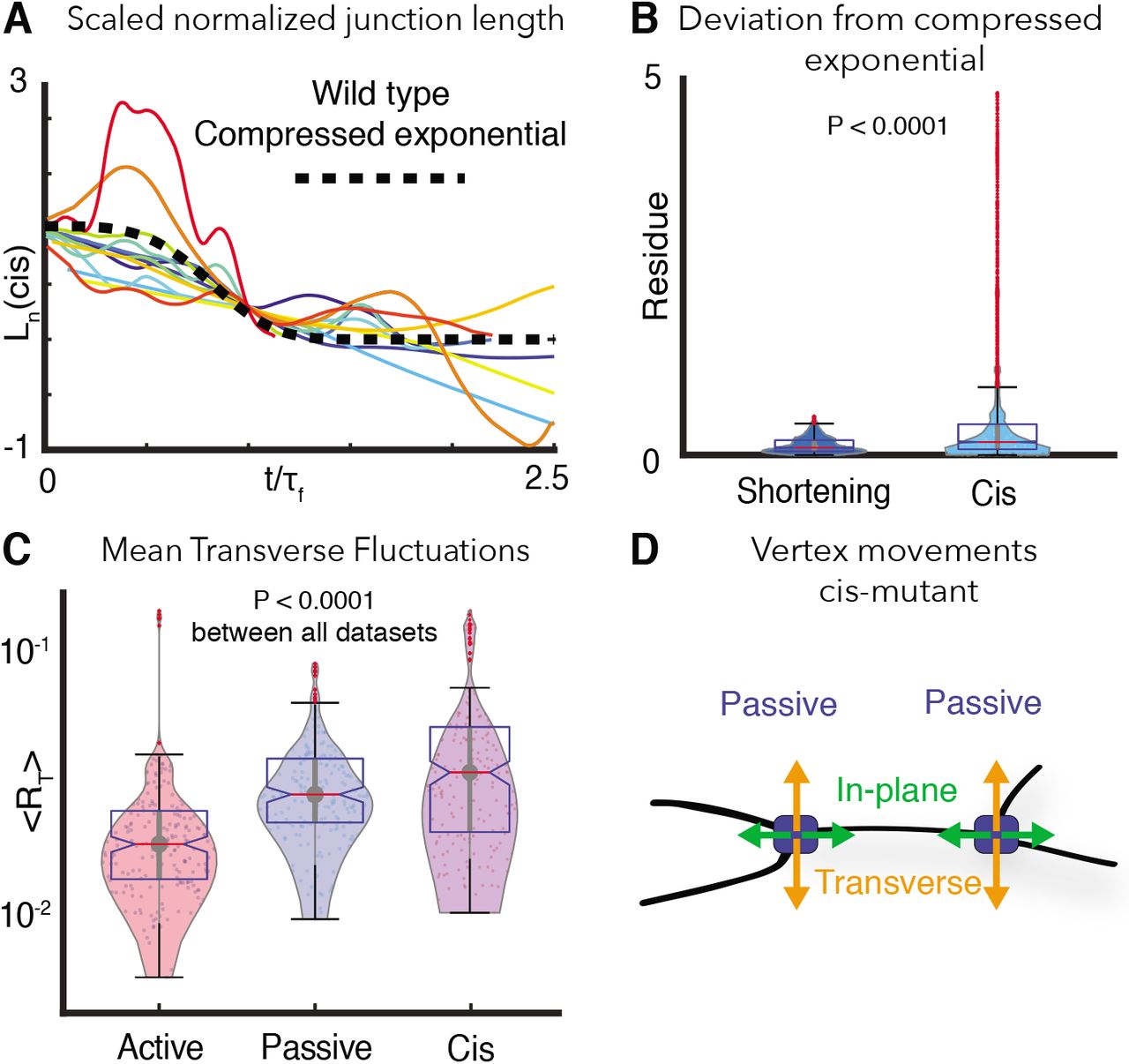
Our theory predicts that the highly localized, asymmetric dynamics observed in vivo result from highly local differences in physical properties along single cell-cell junctions. To test this prediction, we reasoned that the transverse fluctuations of vertices observed in high-speed time lapse data should provide a useful proxy for quantifying very local stiffnesses in vivo (Fig 4A)(SI, Section 16)(43). Indeed, we found that active vertices displayed significantly less transverse fluctuation compared to passive vertices at the same junctions (Fig. 4B, C), suggesting higher local stiffness at active vertices as a consequence of persistent directional motion. In order to validate this idea, we calculated the straightness index of active and passive vertices (SI, Section 16), again finding evidence of more directed motion in active vertices compared to passive vertices (Fig. 4D, E). Thus, both observation and theory suggest that the two vertices bounding shortening v-junctions are molecularly, dynamically, and mechanically asymmetric (Fig. 4F).

A. Schematic of transverse fluctuations in the vertex position perpendicular to the direction of junction shortening. Vertex trajectory is shown as a black line with an in-plane component (green) and an out-of-plane transverse component (yellow). Jumps in the traverse movements are extracted using the transverse “hop” function (see SI, Section 16), inversely proportional to the local vertex stiffness.
B. Violin plots of mean instantaneous transverse fluctuations (“hopping” behavior), 〈RT〉, for active and passive vertices. Active vertex transverse fluctuations are significantly more suppressed compared to passive vertices. The mean is over 10 individual active and passive vertices (total of 20 vertices analyzed from 10 embryos) for vertex movements over 386 seconds. Statistical significance was assessed using t-test.
C. Probability distribution of the vertex transverse fluctuations, RT, for active (red) and passive vertices (grey, offset for clarity) show that the probability distribution peaks at small values of RT for active vertices. Mechanical stiffness of active vertices leads to lesser transverse fluctuations.
D. Straightness index quantifies the persistence of vertex motion in terms of directionality. Active vertices show higher directionality to movement compared to passive vertices in the scatter plot. 20 individual vertices from 10 embryos were analyzed with statistical significance assessed using t-test. See SI, Section 16 for further details.
E. Probability distribution of the straightness index for active (red) and passive (blue) vertices. Probability distribution shows lower persistence to the directionality of motion for passive vertices.
F. Cartoon depicting the relative motions observed at the active and passive vertices decomposed into the inplane and transverse components.
Cis-clustering of Cdh3 in the early embryo is specifically required for axis elongation, but not overall tissue integrity
The findings above strongly suggest that Cdh3 clustering may be a critical node for the control of cell movement during vertebrate CE. Interestingly, while the mechanisms controlling cluster formation have been characterized extensively in Drosophila (25, 26), the functional consequences of clustering remain undefined in any model of CE. For a direct test of the function of Cdh3 cis-clustering, we took advantage of defined point mutations in Cdh3 that specifically disrupt the hydrophobic pocket mediating cis interactions (cisMut-Cdh3; Fig. 5A)(16, 44). To test this mutant in vivo, we depleted endogenous Cdh3 as previously described (Supp. Fig. 6A)(45), and then re-expressed either wild-type Cdh3-GFP or cisMut-Cdh3-GFP.

A. Sketch of the mutations used to inhibit cadherin cis-clustering.
B. Still super-resolution image of cadherin cis-clustering in wild type embryos.
C. Still super-resolution image of the cadherin cis-clustering mutant embryos with endogenous cadherin knocked down (KD). Cis-clusters were absent in this condition and cadherin spatial organization along the cellcell junction shows diffuse structure.
D. Mean spatial autocorrelation of Cdh3 intensity fluctuations for wild type (60 image frames, from 10 embryos) and Cdh3 cis-mutant embryos (56 image frames, 5 embryos). The wild type Cdh3 distribution is organized into well-defined clusters as indicated by the rapid decay in the correlation function. However, spatial organization of cis-mutant cadherin distribution is dysregulated showing a diffuse, gas like spatial distribution along the cellcell junction. This is evident from the gradual decay in the spatial autocorrelation function.
E. Control embryos (~stage 33) showing normal anterior-to-posterior (AP) axis elongation.
F. Sibling embryos in which Cdh3 was knocked down showed a distinct axis elongation defect characteristic of faulty CE.
G. Embryos where endogenous Cdh3 was knocked down and replaced with Cdh3-GFP. The exogenous Cdh3-GFP rescued the AP axis elongation defect observed after knockout of Cdh3.
H. Embryos where endogenous Cdh3 was knocked down and replaced with Cdh3-cis-mutant. These embryos had a clear axis elongation defect showing that the cis-mutant Cdh3 could not rescue the knockdown.
I. Axis elongation was assessed by measuring the animals AP and dorsoventral length, at the widest point, and taking the ratio of these measurements.
J. Embryo cohesion was assessed as the number of embryos that were alive and intact at stage 23.
We first confirmed the cis-mutant’s impact on clustering, again quantifying cluster size using correlation of intensity fluctuations. Importantly, while re-expressed wild-type Cdh3-GFP clustered normally, no detectable clustering could be observed after re-expression of cisMut-Cdh3-GFP (Fig 5B-D; Supp. Fig. 7A)(SI, Section 17). We confirmed this result using multiple methods for quantification (Supp. Fig. 7B-G)(SI, Section 17).
We then used this replacement strategy to examine the function of cis-clustering on tissue morphogenesis in vivo. At neurulation stages, embryos depleted of Cdh3 display severe defects in axis elongation (Fig. 5E, F, I, green)(20, 21). At later stages, these embryos disintegrate due to the widespread requirement for Cdh3 in cell cohesion (45)(Fig. 5J, green). Re-expression of wild-type Cdh3-GFP rescued both axis elongation and tissue integrity, as expected (Fig. 5G, I, J, purple). Strikingly however, while re-expression of cisMut-Cdh3-GFP significantly rescued tissue integrity at later stages (Fig. 5J, red), it failed to rescue axis elongation (Fig. 5H, I, red). These data provide direct experimental evidence that while cisclustering of Cdh3 is dispensable for homeostatic tissue coherence in vivo, it is essential in the more mechanically challenging context of convergent extension.
Cis-clustering of Cdh3 is required for asymmetric dynamics of cell-cell junctions during convergent extension
The specific role for cis-clustering in CE provided a direct experimental entry point for exploring the links between asymmetric vertex dynamics, heterogeneous mechanics, and v-junction shortening. For example, when Cdh3 cis-clustering was disrupted and CE failed, v-junction relaxation patterns also failed to exhibit the normal compressed exponential behavior, displaying large fluctuations instead (Fig 6A, B). In fact, the relaxation pattern of cis-Mut-Cdh3 expressing cells resembled that seen previously in non-shortening junction in vivo and in mechanically symmetrical vertices in silico. This loss of asymmetric dynamics was reflected as well by a loss of asymmetric mechanics, as both vertices displayed significantly elevated transverse fluctuations (Fig. 6C, D). These results suggest that increased cis-clustering near active junctions contributes to increased mechanical stiffness at these sites, which in turn accounts for their distinct dynamics as compared to passive vertices.
A. Ln, the normalized change in cell-cell contact length for cis-mutant embryos. Large fluctuations in junction length is evident similar to non-shortening junctions. Dashed black line indicates the expected compressed exponential behavior.
B. The residue quantifying the cis-mutant junction Ln deviation from the universal compressed exponential function as compared to shortening junctions. Normalized length change of cis-mutant junctions show large deviation from the compressed exponential behavior as opposed to shortening junctions in wild type embryos.
C. Violin plots for mean instantaneous transverse fluctuations, 〈RT〉, for active and passive vertices compared to cis-mutant vertices. Cis-mutant vertices show enhanced transverse fluctuation indicative of reduced local vertex stiffness.
D. Schematic showing all vertices behaved as passive vertices after disruption of cdh3 cis-clustering.
Disruption of PCP signaling disrupts Cdh3 clustering and asymmetric junction dynamics
Finally, we sought to link the observed molecular and mechanical asymmetries to developmental regulatory systems that direct axis elongation. We focused on the Planar Cell Polarity (PCP) genes, which comprise the most well-defined genetic module governing vertebrate CE (46). The encoded proteins are present at shortening v-junctions in Xenopus (Fig. 7A)(47, 48), and while PCP signals are implicated in the control of Cadherin function during CE (22, 23), the mechanisms remain unknown.

A. Sketch of polarized localization of the core planar cell polarity proteins (PCP) dishevelled and prickle. Dishevelled is present on the anterior face of v-junctions and prickle is on the posterior side.
B. Still super-resolution image of Cdh3-GFP in embryos exposed to dominant negative Dvl2 (Xdd1). Cadherin clustering was disrupted after perturbation of PCP.
C. Spatial autocorrelation of Cdh3 intensity fluctuations for Cdh3 with Xdd1 exposed embryos (53 image frames, 5 embryos) and wild type embryos (60 frames, from 10 embryos). Error bar is the standard deviation. The spatial organization of Xdd1 mutant cadherin is similar to cis-mutant embryos showing a diffuse, gas like spatial distribution of Cdh3 along the cell-cell interface.
D. Ln, the normalized change in cell-cell contact length for Xdd1 embryos. Large fluctuations in junction length is evident similar to non-shortening and cis-mutant junctions. Dashed black line indicates the expected compressed exponential behavior.
E. The residue for the Ln deviation from the universal compressed exponential function for Xdd1 junctions as compared to shortening junctions. Normalized length change of Xdd1 junctions show large deviation from the compressed exponential behavior as opposed to shortening junctions in wild type embryos.
F. Violin plots for mean instantaneous transverse fluctuations, 〈RT〉, for active and passive vertices compared to Xdd1 vertices. Xdd1 vertices show enhanced transverse fluctuation indicative of reduced local vertex stiffness similar to cis-mutant vertices.
G. Schematic summarizing the primary conclusions: (i) we identify the asymmetry in vertex movements that contribute to junction shortening during CE. Active vertices move more and mainly contribute to junction shortening while passive vertices move less. (ii) We discover that cadherin cis-clustering is the driving mechanism in determining which vertex is active versus passive. (iii) Cadherin cis-clustering locally increases the viscoelastic parameter near active vertices thereby stabilizing the vertex movement in the transverse direction. This allows for active vertices to contribute to junction shortening. Passive vertices, cis-mutant vertices and Xdd1 vertices are characterized by enhanced transverse movement.
We disrupted PCP with the well-characterized dominant-negative version of Dvl2, Xdd1, which severely disrupts CE (28). Strikingly, expression of Xdd1 elicited a clear disruption of Cdh3 clustering, similar to that observed for cisMut-Cdh3 (Fig. 7B, C). Xdd1 also disrupted the compressed exponential behavior of v-junction shortening, with junctions exhibiting large fluctuations in length reminiscent of those observed normally in non-shortening junctions in vivo and in silico (Fig. 7D, E). Finally, vertices in Xdd1-expressing cells did not display asymmetric dynamics, and both vertices displayed elevated transverse fluctuations indicative of reduced stiffness (Fig. 7F). These data link PCP protein function, Cdh3 cis-clustering, local mechanics, and effective cell movement during vertebrate CE.
Discussion
Here, we combined physical and cell biological approaches to observation, theory, and experiment to identify and link two novel features of vertebrate convergent extension, one physical, the other molecular. First, we show that even individual cell-cell junctions display asymmetric physical and mechanical heterogeneities during CE. Second, we show that locally patterned cis-clustering of a classical cadherin is required for these heterogeneous behaviors. These results thus provide fundamental new insights into both the physics and the biology of convergent extension, the evolutionarily conserved process that shapes the early embryo of nearly all animals.
From a physical perspective, this work provides the first evidence for mechanical heterogeneity along individual cell-cell junction in an intact, living animal in vivo. This work is important not only for expanding the biological context of similar findings in single cells in culture (16–18), but also for providing a link between the poorly defined subcellular mechanics of vertebrate CE and the more well defined tissue-scale physical features (5–8). In considering this multi-scale mechanical nature of CE, a major unresolved question relates to the origin of asymmetry between passive and active vertices, which is a conserved feature of Drosophila epithelial cells (29) and Xenopus mesenchymal cells (Fig. 1). One attractive possibility is that this asymmetry represents an emergent property of tissue level mechanical force balance in the tissue. Given the success of previous vertex models for understanding such tissue scale properties (12–15, 36), incorporation of the physical properties described here into those existing frameworks should be highly informative.
In addition, these mechanical findings provide new cell biological insights into a unifying suite of cell behaviors that is deeply conserved across evolution (1). V-junction shortening is accomplished by a combination of cell crawling via mediolaterally-positioned lamellipodia and active contraction of anteroposteriorly-positioned cell-cell junctions (1), a pattern that has now been described in nematodes (49), insects (50–52), and vertebrates (11, 27, 53). Our analysis of vertices was indifferent to the contributions of crawling and contraction, so it is remarkable that the relaxation behavior in Xenopus nonetheless can be scaled to the unified pattern described by a compressed exponential (Fig. 1). This result argues that the contribution of crawling and contraction is likely to be continuously integrated in all V-junctions during Xenopus CE, a conclusion that would help to unify previously incongruent findings in this important model organism (e.g. (11, 27)). Finally, it remains to be determined whether v-junction shortening in Drosophila epithelial cells also displays glassy dynamics and a compressed exponential relaxion, but it is nonetheless remarkable that even subtle aspects (e.g. active and passive vertices) are similar in Drosophila epithelial cells (29) and in Xenopus mesenchymal cells (Fig. 1). Further application of physical methods for exploring motion in these systems should be highly informative.
Another substantial impact of this work relates to our understanding of classical cadherin functions during collective cell movement. First, our data suggest that the tuning of very local mechanics by cadherin clustering allows one vertex to limit the glass-like state, thus entering a more fluid-like state, and thus exhibiting persistent motion to shorten the v-junction. In addition, though cadherins comprise a large family of related molecules, the vast majority of work has focused on a single molecule, Cdh1 (aka E-cadherin)(19); our work on Cdh3 in vertebrate mesenchymal cells therefore provides a long-overdue complement to the extensive previous work on Cdh1 in Drosophila epithelial cells (24, 25). Though this may seem a minor point, the issue is actually highly significant, because while the cell behaviors are conserved, Drosophila CE does not require PCP proteins (54). As such, the data here should provide important insights into the interplay of PCP and cadherins in other vertebrate tissues, such as the skin, which also strongly expressed Cdh3 (mouse P-cad) and undergoes PCP-mediated CE (55).
Finally, our findings on cadherin clustering are also important. Lateral clustering was first described for cadherins over two decades ago (41, 56), and the cis-clustering mutants used here were rationally designed based on the Cdh1 and Cdh3 crystal structures (44). While studies in cell culture indicated a role for cis-clustering in the formation of stable adhesions and coordination of cell collectives (16), our data here nonetheless represent the first in vivo test of clustering requirements in any intact animal. Given the links between CE in human neural tube defects, our results here provide a biomedically relevant biological context for understanding the function of cis-clustering of classical cadherins and moreover reveal local, planar patterning of cis-clustering as an additional regulatory node linking molecules to mechanics during vertebrate axis elongation
Theory Supplement
Section 1. Active versus passive vertex dynamics
We used the Manual Tracking plugin in FIJI to obtain the trajectories of vertex pairs. Individual vertex positions were tracked for a time interval of 400 s. By obtaining the time-dependent two-dimensional (2D) vertex co-ordinates (xL, yL) and (xR,yR) for the left (L) and right (R) vertices respectively, the net distance travelled by the left(L) vertex is,
 where xL(tf), xL(t0) are the vertex positions at the final (tf) and initial time (to) of measurement respectively. A similar equation with xR,yR applies for the right vertex. The length of the junction is,

To determine the weight of the contribution of each vertex to junction shortening, we define an activity parameter, A, as the ratio of net vertex distance moved to the initial junction length i.e.  . Similarly,
  , for the right vertex. If AL > AR, the left vertex is labelled as the ‘active’ vertex while the right vertex is the ‘passive’ one, and vice versa if AR > AL. Over the time frames that we have analyzed the vertex movement, the median value of L(tf)/L(t0)~0.30, implying that the junctions have shortened by ~ 70%. Both high time resolution and low time resolution imaging data show the same trend that one of the vertices tend to be more active, contributing more to junction shortening (Fig 1B-C, Main Text). We confirm that this observation is not due to the overall translation or rotational motion of the cells as detailed below (Supp. Fig. 2).
Section 2. Normalized junction length dynamics
We calculated the normalized cell-cell junction contact lengths to characterize the selfsimilarity in the length change underlying cell neighbor exchanges during convergent extension. We selected all cell-cell contacts that shorten over time intervals > 100s, and normalized the change in length as,
 where L(tf), L(t0) are the junction lengths at the final and initial time points respectively. The normalized junction length dynamics, Ln(t), provides insight into the active processes that underlie vertex movement driving CE. Since junction lengths are highly heterogeneous (Fig 1D, Main Text) relative to, L(t0), and the time to closure, tf – t0, the normalization in Eq. (3) allows us to rescale all the length changes to values between 1 and 0. The normalized length curve was smoothed (over 10-time frame windows = 20s) to remove high frequency noise. To determine if junction shortening exhibits a self-similar behavior across multiple embryos, we rescaled the time axis in Ln(t) by the relaxation time τf, defined as the time at which Ln(t = τf) =0.3. This corresponds to a 70% change in the junction length. Rescaling the time axis by t/τf collapses the normalized lengths onto the functional form,
 which is a single compressed exponential (Fig 1E, Main Text). The extent of the self-similarity is striking in comparison to both non-shortening (Fig 3E, Main Text) and cis-mutant normalized junction lengths (Fig 6A, Main Text). Notice that for t < τf, change in normalized junction length is slower than exponential decay. However, for t > τf, normalized junction length significantly shortens faster than would be predicted based on exponential decay. Therefore, the compressed exponential behavior for Ln provides evidence that the persistence of junction shortening increases with time.
Section 3. Junction length fluctuations
To analyze the instantaneous change in the junction length, we calculated, δL(t) = (L(t) – L(t + δt)), where δt = 2s and t is the time. The unit of the length fluctuations is μm. When the junction shortens, δL(t) > 0, while extension implies δL(t) < 0 (Fig. 2D, Main Text).
The probability distribution of δL is plotted in Suppl. Fig 3D. We observe increasing persistence of junction shortening as a function of time, an indication of a positive reinforcement that enables more persistent junction shortening. To quantify the trend in increasing persistence of junction shortening, we classify the instantaneous length change, δL(t), into two stages – early and final stages of junction shortening. Early stage is defined as the first 0.2 * Nframes, where Nframes is the total number of time frames over which junction length data is collected. The final stage is defined as the time frames > 0.8 * Nframes. The junction length fluctuations and its mean (red and black lines at early and final stages respectively) become more positive (δL(t) > 0) from the initial to the final stage (Suppl. Fig 3D, orange for the early stage and blue for the final stage), which provides evidence that junction shortening is more persistent as time increases.
Section 4. Quantifying the heterogenous dynamics of vertices: Mean Square Displacement (MSD), van Hove function and the velocity autocorrelation
The characteristics of vertex dynamics could provide clues as to the active mechanisms that promote or impede vertex movement. An important parameter to quantify vertex dynamics is the Mean Square Displacement (MSD), as a function of the lag time t. Time averaged MSD,  , is calculated using the vertex positions
  ,
,
 where T = 400s and subscript L stands for the left vertex. Taking the average over N independent vertex trajectories, labelled by the index i, the ensemble averaged MSD,
 . The same procedure is used to calculate the MSD for the right vertex (see Fig 1F, Main Text). In many physical systems the MSD increases with a power law, i.e. Δ(t)~tα. When uncorrelated and random Brownian motion occurs, the MSD exponent is unity, α=1. Sub-diffusive, α<1, movement occurs when there is a hindrance to motion or the dynamics is highly correlated. For example, when a particle in caged by its immediate neighbors, sub-diffusive motion results. Super-diffusive MSD, α>1, is seen when the motion is highly directed.
We found substantial heterogeneity in individual vertex MSD as seen from the plot of  (Suppl. Fig 2A). Active and passive vertex MSDs span 3 orders of magnitude of time lag. Two distinct time regimes are observed for both active and passive vertex movements: (i) at short time lags, t < 30s, active and passive vertex movements are random, characterized by MSD exponent α~1. (ii) For t > 40s, active vertices show strong superdiffusive movement while passive vertices undergo a slowdown followed by a recovery towards superdiffusive motion (see Fig 1F, Main Text). These distinct differences between active versus passive vertices are observed in the ensemble averaged MSD, Δ(t) for 20 vertices from 10 different embryos.
To eliminate the effect of translation and rotational motion of the entire tissue, we tracked vertex positions with respect to the center of an egg yolk particle (Suppl. Fig 2) typically present within cells as well as nearby stationary vertices (Suppl. Fig 2). In this manner, we analyzed the relative vertex distances,  , with respect to a frame of reference within the tissue that is being imaged. By extracting the co-ordinates of the center of an egg yolk within a cell or nearby vertices,
  , we obtain the relative vertex positions,
  . We then evaluated the mean square relative displacements (MSRD) for the left and right vertex pairs using Eq. (5) above. The distinct differences between active versus passive vertex dynamics is conserved in this relative co-ordinate system, indicating that the asymmetry in active versus passive vertex movement is not due to translational or rotational motion of the whole tissue (see Suppl. Fig 2).
Van Hove Function
Insights into vertex motion may be obtained by analogy to spatially heterogenous dynamics in supercooled liquids [1,2]. The distribution of particle displacements is expected to be a Gaussian in simple fluids. In supercooled liquids, however, the displacements of a subset of particles deviate from the Gaussian distribution [1]. From the distance moved by a vertex during the time interval δt, defined as  , the van Hove function for vertex displacement (or the probability distribution of vertex step size) is,
 where the average is over N independent vertex trajectories. The van Hove distribution at δt = 40s, for active (red) and passive vertices (blue) is shown in Suppl. Fig 4A. The 40s time interval is long enough to clearly observe the differences in the distances moved by active and passive vertices. The van Hove distribution at δt = 4s is shown in Suppl. Fig 4B. At this short time interval, distances moved by active and passive vertices are similar and is well fit by a Gaussian (see inset Suppl. Fig 4B). However, the van Hove distribution deviates significantly from the Gaussian distribution at δt = 40s (see inset Suppl. Fig 4A), indicating the growing heterogeneity in the displacements.
Average velocity distribution and velocity autocorrelation function (VACF)
To further quantify the striking differences in the movement of active and passive vertices, we calculate the average velocity of the vertices. The average velocity over a time interval τ is defined as,

Replacing  by
by  gives the average velocity of the right vertex. We analyze the average velocity over a time interval τ because experimental data is also an average over the time resolution of the iSIM microscope. We then compare the speed distribution
  of active and passive vertices over both short, τ = 4s (Suppl. Fig 4C, blue for passive and red for active vertices) and longer time intervals, τ = 60s (Suppl. Fig 4D). At the smaller time interval, τ = 4s, the speed distribution of active and passive vertices are similar. This indicates minimal differences between active and passive vertex dynamics at this short time scale. The difference in active and passive speed distribution is, however, pronounced at τ = 60s. The passive vertex speed distribution peaks at a smaller value and decays rapidly for larger speed values, compared to active vertices. This illustrates the fluidization in the movement of active vertices that develops over a time scale of order 50s. This agrees with other measures such as the MSD and the van Hove distribution as reported above.
To probe the time interval over which the average velocity (at fixed τ) is correlated with average velocity at a time point separated by δt, we calculate the velocity autocorrelation function (VACF),
 where the average is defined as
  . The VACF is normalized such that
  . At the shorter time interval of τ = 4s, VACF for active and passive vertices exhibit a rapid decay to zero (Suppl. Fig 4E, blue for passive and red for active vertices). Individual vertex VACF are plotted in transparent colors and the mean as dashed lines (blueblack dashed line for passive vertices and red-black dashed line for active vertices). Analyzing vertex velocities at τ = 60s clearly brings out the different dynamics that characterize active versus passive vertices (Suppl. Fig 4F, blue for passive and red for active vertices). Velocity correlations decay quicker for passive vertices, becoming negative and then rebounding to positive values. However, active vertex velocity correlations are more persistent with time as evident from the longer time to decay.
Section 5. Self-overlap parameter and dynamic heterogeneity
To quantify the highly asymmetric vertex movement that underlies CE, we measured the fractional change in vertex positions over a time interval t using the self-overlap order parameter, defined as:
 where
where  and wi = 0 otherwise. The self-overlap parameter is dependent on the length scale that is probed by Lc. We chose Lc = 1.3μm, as this is the distance scale over which movement of active and passive vertex become distinct. This is evident from the plot of MSD (Fig 1F, Main Text) for active and passive vertices where the dynamics begins to differ at a length scale of > 1μm. If a vertex moves less than Lc = 1.3μm over the time interval t, the vertex is considered to have 100% overlap with its previous position, and hence assigned a value 1. However, if the vertex has moved more than 1.3μm within the time interval t, we consider this as 0% overlap. The self-overlap function, 〈Q(t)〉, is calculated by averaging over a range of initial times, t′, followed by ensemble averaging over individual vertices (Fig 1G, Main Text). The active vertex self-overlap function decays rapidly and can be fit to a single exponential decay function, indicating liquid like dynamics. However, passive vertex overlap function shows a two-step decay, a signature of glass-like dynamics (Fig 1G, Main Text).
Although the MSD and the self-overlap function 〈Q(t)〉 are useful to quantitatively characterize vertex movement, other metrics are needed to gather further insights into the dynamic heterogeneity and correlations in vertex movement that emerge temporally during CE. In systems approaching the glass transition, the cooperativity of motion increases such that the length and time scales characterizing the dynamic heterogeneity are expected to grow sharply. In supercooled liquids, the fourth order susceptibility, Χ4(t), provides a unique way to distinguish the dynamic fluctuations between liquid and frozen states [3]. Therefore, we compute the fourth order susceptibility from the variance of the self-overlap parameter, Χ4(t) = 〈Q(t)2〉 – 〈Q(t)〉2

Similar to structural glasses, the dynamic heterogeneity, quantified by Χ4(t) increases with time, peaks at a maximum time interval, tM and then decays (Fig 1H, Main Text). The dynamic heterogeneity is manifested as dramatic variations between individual vertex trajectories in both active and passive vertex movements. For active vertices, Χ4(t) peaks at tM~120s while for passive vertices heterogeneity peaks at a longer time interval tM~170s (Fig 1H, Main Text). The time scale associated with the peak in dynamic heterogeneity is consistent with the viscoelastic relaxation time (further discussed below), known to be the characteristic relaxation time for vertices connected by the cell cortex under tension [4]. For non-shortening junctions, Χ4(t), does not show a peak (Suppl. Fig 4H). We anticipate the peak to be at a much longer time scale for vertices of non-shortening junctions.
Section 6. Cadherin clustering from the spatial autocorrelation function
To determine the characteristic spatial correlation of cadherin intensity fluctuations, we analyze the pixel-by-pixel Cadherin3 (Cdh3) intensity data,  , along the medio-lateral cell-cell interface (v-junction). Here,
  is the position vector of the i-th pixel in the iSIM image. The spatial autocorrelation function of the cadherin intensity fluctuations as a function of distance, r, along the cell-cell interface is,
 where θ(z) = 1 if z = 0, θ(z) = 0 for any other value of z. 〈I〉 is the mean cadherin intensity over all the pixels in the cell-cell junction. C(r) is normalized such that C(r = 0) = 1. The cadherin correlation length is defined as the distance, ξ at which C(r = ξ) = 0. This provides a measure of the distance scale at which the correlation in cadherin intensity fluctuations is lost. Equivalently, ξ, sets the spatial persistence of cadherin fluctuations along the cell-cell junction, providing a quantitative measure of lateral cadherin clustering. We analyzed each cell-cell junction separately and obtained the spatial correlation behavior for individual junctions from multiple embryos. The mean of the cadherin spatial correlation (over multiple time points) for wild type embryos is reported in Fig. 2C, Main Text with the error bar denoting the standard deviation. To analyze the dynamic variation in cadherin cluster size as a function of time, C(r), was calculated at multiple time points (over a time interval of 320s). The fluctuation in cluster size is given by, δξ(t) = ξ(t) – 〈ξ〉t, where 〈ξ〉t is the mean cluster size over the analyzed time interval (see Fig. 2D Main Text). The cluster size fluctuation, δξ(t), was smoothed (over 10-time frame windows = 20s) in order to remove high frequency noise.
Section 7. Cross-correlation between cadherin cluster size and the junction length fluctuations
The normalized cross-correlation between junction length fluctuations, δL(t), and cadherin cluster size fluctuations, δξ(t), was calculated in MATLAB using,
 where T is the total time of analysis and τ is the lagtime. We analyzed the cross-correlation for 18 junction shortening events and show the correlation coefficient as a heatmap in Fig 2E Main Text.
Section 8. Asymmetry in cadherin clustering
To quantify the asymmetry in Cdh3 clustering in the spatial region near the left and right vertices, we calculated the spatial correlation in cadherin intensity fluctuations, C(r) (see Eq. (11)), in a region spanning 3.25μm adjacent to left and right vertices. The spatial region is chosen such that on average it is 3X larger than typical cadherin cluster size of order 1μm. The localized cadherin clustering behavior adjacent to active and passive vertices, quantified by the spatial correlation in cadherin intensity fluctuations, is shown in Fig. 2F Main Text. Fig 2G, Main Text shows the local cadherin clustering behavior for non-shortening junctions. Cadherin clustering is enhanced near active vertices as opposed to passive vertices in shortening junctions (Fig. 2F Main Text) while it is symmetric near left and right vertices in non-shortening junctions (Fig. 2G Main Text).
We used an alternative definition of C-cadherin cluster size to confirm our results. By fitting the decay in cadherin spatial autocorrelation function to zero by an exponential function,  , we can extract the cluster size ξ. We find that the asymmetry in the local cadherin clustering behavior is independent of the definition of the cluster size (Suppl. Fig 5B-C).
Section 9. Theoretical Model
Vertex based models are important for studying the dynamics of confluent cell layers [5]. The junction between three or more cells (vertices) are represented as point particles. The connecting edge between vertices represent cell-cell interfaces. We developed a theoretical model for junction shortening to understand the asymmetric dynamics of vertices. Our model, shown in Fig 3A-B Main Text, is a coarse-grained representation of a collection of cells intercalating mediolaterally. Each vertex, bounding the v-junction, are connected to Maxwelllike components with viscous and elastic elements. Elastic properties are modelled by springs with stiffness, k, and actuators characterize the viscous motion of cell vertices (see Fig 3A Main Text; γ is the viscosity). For the purposes of visualization, we depict the spring-actuator element as being in the direction away from the cell-cell interface, exerting a compressive force on the vertices. This need not be the case as the forces and mechanical factors contributing to junction shortening can also be localized within the cell-cell junction. For the purposes of simplicity in visualization, we have picked a direction for the spring-actuation element.
We assume that the position of the left vertex,  , evolves according to the equation of motion:
 where
where  is the elasticity of the left (L) vertex,
  is the contractile force responsible for viscous deformation of the vertex and γL is viscosity coefficient of the vertex. Replacing the subscript L with R above gives the equation of motion for the right vertex. The local elasticity near the vertices are accounted for by a connected harmonic spring with strength
  . The spring is connected in series with an actuator that supplies the contractile force,
  . It is likely that the noise in a physical or biological system is correlated in time. Consistent with our observation that fluctuations in junction length are correlated in time (Suppl. Fig 4I), we model ζL as the colored noise experienced by the vertices. The noise, ζL, represents the coupling of the vertices to their immediate local environment, satisfying 〈ζL(t)ζL(s)〉 = Ae−|t−s|/τn with the mean 〈ζL(t)〉 = 0. The coefficient, A, is the noise strength. For large noise strength, vertex positions show large amplitude deviations from the position dictated by the minimum of the elastic force, as constrained by the spring. For small persistence time of the correlated noise, τn, the vertex dynamics is highly uncorrelated in time. At large persistence times, however, the noise induced fluctuations in the vertex positions are correlated over the timescale τn. We set the noise correlation time to be the persistence time of junction length fluctuations (Suppl. Fig 4I). The colored noise satisfies,
  , where η(t) is the Gaussian white noise source characterized by delta correlation 〈η(t)η(s)〉 = δ(t – s) and mean 〈η〉 = 0.
Since the movement of vertices along the medio-lateral direction is much more persistent as opposed to the perpendicular direction, as evident from the closure of junctions, we simplify the model to consider only one-dimensional (1D) motion. Henceforth, we drop the vector notation and focus on the vertex dynamics along the x-axis.
By considering the basic vertex equations in the Langevin picture,

 we model the vertex equations of motion in analogy to particles moving in a translating optical trap. The minimum of the left elastic ‘trap’ changes dynamically due to the term aLtψL in Eq. (14) (modelled by the left dashpot). Similarly, the right elastic ‘trap’ is translated from its initial position L0 by aRtψR in Eq. (15) (modelled by the right dashpot). These terms serve as a proxy for active contractile forces which viscously deform the cell edges. Hence, we refer to the exponents, ψL and ψR, as the yield exponents. The physical implication of the yield exponent is that the rest length of the junction varies dynamically. The contractile force is,
  in Eq. (13), where V(xL) is the time dependent ‘trap’ potential of the form VL = 0.5kL(xL – aLtψL)2 and
  The stochastic movement of the vertices in a translating potential leads to a ratchet-like effect where the vertex dynamics has a specified direction. This directionality in the motion of the vertices does not arise, however, from the asymmetry in the potential but rather from the asymmetric translation of the potential well minimum.
Hence, the active forces contributing to junction shortening were modeled in silico as,

 where aL and aR are the ‘acceleration’ of the left and right vertices respectively, and the exponents ψL and ψR determine the temporal dynamics of the contractile force. We include the acceleration term to account for the experimentally observed increase in the persistence of junction shortening as a function of time (see Fig 1D-E Main Text). The initial condition is set as xL(t = 0) = 0, and xR(t = 0) = L0, with L0 being the initial edge length. We arbitrarily assign the left side to be active, with the time dependent active force rising in proportion to tΨL(ψL > ΨR). The right side is assigned to be passive, with force increasing with time as ∝ tΨR. The difference in the yield exponents, ψL versus ψR, determines which vertex is active. The equations of motion then become:


Defining  and
and  , where x0 = 10μm, τ = 102 sec and
  , we recast the equations of motions into dimensionless forms. Similar normalization with L replaced by R applies for the right vertex. The system of equations is scaled with the characteristic length and time, x0 and τ, physiologically relevant for cells undergoing convergent extension. In terms of the normalized quantities, the equation of motion is,

 where the parameter
  has the dimension of inverse time
  . When normalized by the characteristic timescale τ,
  , we obtain a dimensionless parameter which we refer to as the viscoelastic ratio.
Section 10. Dynamic rest length and colored noise
In vertex-based models for plant cells, the cell-cell interface length is modeled with a spring having a characteristic rest length [6]. Any deviation in the length of the cell-cell interface from the rest length is energetically unfavorable. In vertex models for animal cells, such a rest length is typically not included [5]. In our coarse-grained vertex model, we include a spring term with dynamic rest lengths. We show that this model accounts for the asymmetric vertex dynamics and quantitative experimental features of the junction shortening behavior. By studying actomyosin contractility in combination with theoretical modeling, it has recently been shown that epithelial junctions exhibit both elastic and viscous remodeling behavior [7].
The existence of memory effects in junction shortening necessitates the addition of the colored noise term. Previous vertex-based models have considered random white noise indicating no memory effect. However, by experimentally quantifying the junction length fluctuations, we would like to point out that colored noise may be important to consider in modeling biological systems.
To determine the characteristic timescale of the fluctuations in cell-cell junction length, δL(t), we calculated its temporal autocorrelation,

Each average  , was calculated for data in the time range (0,T – δt) with T being the duration of the experiment and δt the lag time. The autocorrelation is normalized such that CδL(δt = 0) = 1. The length fluctuation correlation for individual cell-cell junction from multiple embryos was calculated separately (Suppl. Fig 4I). The thickness of the black line accounts for the standard deviation. The persistence time of junction length fluctuations (~13s) is obtained from fitting the mean correlation function, CδL(δt), to an exponential (see Inset Suppl. Fig 4I).
Since the junction length dynamics is persistent over a time scale of ~10s, we surmise that the dynamics of vertices at two different time points is correlated i.e. memory effects become important. This motivates the need for additive colored noise in the equations of motion of the vertices. The persistence time of the colored noise is set by the persistence time of the junction length fluctuations, as we discuss in detail below.
Section 11. Parameter values for elasticity and viscosity
The viscoelastic ratios,  and
and  , were varied from 0.05 to 5 equivalent to 5 × 10⁻⁴s−1 – 0.05s−1 in dimensional units. Therefore, the viscoelastic relaxation time is in the range of 20s – 2000s. Spring stiffness, k, in the range between 100pN/μm and 1nN/μm [8,9] and the viscosity, γ ~100nN.s/μm [10], accounts for the elastic and viscous properties of tissues previously reported in the literature. For these values, one obtains the viscoelastic relaxation time in the range of 1s – 100s. Therefore, the viscoelastic ratio used in our model is within an order of magnitude of the physiological values for both tissue stiffness and viscosity.
Section 12. Simulation Details
We consider a wide range of values for both the viscoelastic ratio and the yield exponent for the active vertex, ψL. The time step in the simulation is Δt = 0.0022 = 0.22s, chosen to be smaller than the characteristic viscoelastic relaxation time (of order 10s). We evolve the simulation for a total of n=20,000 steps (4,400s in real units). The equations of motion are solved using the Euler method for each vertex. If at any point during the simulation, the left and right vertex positions approach one another to a distance less than 0.5μm, we label the junction as having successfully completed the shortening. The initial junction length was set to be L0 = 2, equal to 20μm in real units. The range of yield exponents we consider is limited by the need to ensure that the minima of the potentials do not overlap during a given simulation run. To generate the phase diagram for the probability of junction shortening as a function of the yield exponent and the viscoelastic ratio, we consider for the left active vertex  at intervals of 0.5. Yield exponents in the range, 1.7 < ψL < 2, were simulated at intervals of 0.25 for the active vertex. ψR = 1.3 is fixed for the passive right vertex. The acceleration of the potential minima, is set to be āL = āR = 0.001. The viscoelastic ratio for the right passive vertex is fixed at
  . We simulated 100 junction shortening events at each value of the parameters
  and ψL. By monitoring the percent of successful junction shortening events, we generate the phase diagram in Fig 3C (Main Text).
Section 13. Effect of viscoelasticity on the shortening of junctions
We observe in the phase diagram (Fig 3C, Main Text) that at a fixed value of the yield exponent, modulating the viscoelastic parameter leads to a transition from non-shortening to junction shortening regime. At constant ψL = 1.95, for low values of the active vertex viscoelastic parameter,  , less than 40% of the junctions shorten. However, at higher values of the viscoelastic parameter,
  , more than 80% of the junctions successfully execute shortening. Therefore, the theory predicts that the local viscoelasticity is critical for cells to intercalate medially and effect convergent extension. We calculate the normalized length for non-shortening junctions and found that the self-similarity in junction length dynamics is broken, in agreement with experimental results (Fig. 3E, Main Text). Ln for non-shortening junctions is characterized by large fluctuations away from the expected compressed exponential behavior, as quantified by the residue (see details below). Simulated junction length dynamics for the non-shortening case (grey curves in Fig 3E Main Text) is obtained for parameter values
  and ψL = 2, ψR = 1.3. Meanwhile, for the shortening phase (grey curves in Fig 3D Main Text),
  and ψL = 2, ψR = 1.3. Therefore, asymmetry in viscoelasticity is critical for junctions to execute shortening. Our model points out that the persistent dynamics of active vertices, enabling the efficient shortening of the cell-cell interfaces, is a direct consequence of the faster viscoelastic relaxation time.
Section 14. Residue
We quantify the deviation of the normalized junction shortening from the expected compressed exponential behavior by calculating the rescaled time,  , and
, and  , where ω is the residue. τy, is defined as the time at which Ln(t = τy) =0.3.
In Fig 3F (Main Text), non-shortening junctions show strong deviations from the expected compressed exponential behavior while shortening junctions closely follow the compressed exponential form.
Section 15. Alternative form of the contractile force
To test the robustness of the conclusions obtained using our model, we consider an alternative form of the contractile force experienced by the vertices. We model the actuators contributing to viscous junction shortening as moving with constant velocities -  and
and  - for the left and right vertices respectively:


The ‘trap’ potential in this scenario is of the form, VL = kL(xL – vLt)2 and VR = kR(xR – (L0 – vRt))2, moving with constant velocities. Left vertex is defined to be active with  The velocity is normalized as
  . The passive vertex velocity is fixed at
  , which in dimensional units correspond to 0.0011μm/s. The active vertex velocity is varied in the range of
  , which in dimensional units is between 0.003μm/s −0.0034μm/s. Experimental vertex shortening velocities in the range of 0.001μm/s to 0.021μm/s was reported by some of us in a previous work [11]. Fixing the passive viscoelastic ratio at,
  , we varied
  for the active vertex. Keeping all the other parameters the same, we arrive at the same conclusion that local junction viscoelastic response is critical to effect junction shortening (Suppl. Fig 4J). Therefore, our conclusions are not affected by the specific form of the vertex dynamics. A crucial aspect is that the two potential well minima should move asymmetrically in time.
Section 16. Transverse fluctuations of the vertices
We quantify the intermittent movement (see Fig 4A Main Text) of the vertices perpendicular to the motion that contributes to the junction shortening by calculating the transverse fluctuations, RT. The transverse step size is given by,  , where
  and the angle θ is the obtained from the dot product,
  . Here, the net displacement of the Left(L) vertex is given by,
  . Similar equation applies for the right vertex with xL,yL replaced by xR,yR. To better quantify the intermittent dynamics, we compute the transverse “hop” function,

The angular bracket above 〈..〉B denote the average over the time window  . We chose for the hop duration parameter, δt = 4s, to probe short time transverse fluctuations. The probability distribution of all Rτ(T) values are shown in Fig 4C Main Text. By averaging the transverse fluctuations over all vertices,
  , we obtain the mean transverse fluctuation for active and passive vertices (Fig 4B Main Text). 〈RT(t)〉 for Cis-mutant and Xdd1 vertices are shown in Fig 6C and Fig. 7F of the Main Text respectively.
Straightness Index
The directionality of the vertex trajectories were assessed using the straightness index. This is defined as the ratio of the net distance moved by a vertex between initial and final time points to the total distance moved by a vertex:

Higher the value of the straightness index, the more directed the movement is with the value of straightness index = 1 indicating perfectly straight line motion.
Section 17. Perturbation of Cadherin clustering in individual junctions and its spatial periodicity
We calculate the spatial autocorrelation of the cadherin intensity fluctuations (C(r) see Section 6, Eq. (11)) for four different embryo development scenarios, (i) wild type Cdh3 (see Fig. 2C, Main Text), (ii) Cdh3 rescue (Cdh3-GFP) (see Suppl. Fig 7A), (iii) Cdh3 cis-mutant (cisMut-Cdh3-GFP) (Fig. 5D, Main Text), and (iv) Xdd1 (Fig. 7C, Main Text), from multiple embryo samples. The mean spatial correlation in cadherin fluctuations for wild type Cdh3 and Cdh3-GFP junctions show similar behavior with the decay to zero characterized by an exponential form (Suppl. Fig 7B). The exponential spatial dependence is evidence for the existence of a characteristic spatial scale for correlations in cadherin spatial distribution. The local peak in the cadherin autocorrelation function is identified using the findpeaks algorithm in MATLAB. Local peak in a data array is identified when a data point is larger than its two neighboring data points or equal to infinity. By setting the prominence of the peak to 0.1, we identify how the peak amplitude stands out relative to other peaks. Wild type and rescue embryo cell-cell junctions are characterized by well-defined spatial periodicity in cadherin clustering, as observed from the secondary peaks in the spatial correlation (see black triangles, Suppl. Fig 7C). Therefore, cadherin spatial organization in wild-type Cdh3 and Cdh3-cis-mutant rescue embryos is in a crystal-like phase (Suppl. Fig 7C), with regularly repeating spatial patterning. Cadherin spatial correlation for individual frames (with no averaging) is shown for control (solid lines in Suppl. Fig 7D) and cadherin rescue embryos (dashed lines, Suppl. Fig 7D). However, cadherin spatial correlation in Xdd1 and cisMut-Cdh3 embryos shows a diffuse spatial organization, with little to no secondary peak structures visible in the spatial autocorrelation (see Suppl. Fig 7E). This is indicative of disrupted periodicity in cadherin clustering. Therefore, cadherin spatial organization in cisMut-Cdh3 and Xdd1 embryos is in a gas-like phase. Individual frame cadherin spatial correlation for cisMut-Cdh3 (solid lines Suppl. Fig 7F) and Xdd1 is shown as dashed lines in Suppl. Fig 7F. For Xdd1 and cisMut-Cdh3-GFP junctions, the decay in the spatial correlation is better fit by a power law, indicating the lack of existence of a coherent length scale associated with fluctuations in cadherin expression (Suppl. Fig 7G).
Section 18. Statistics
The statistical test used and other relevant details such as the number of embryos/image frames analyzed are described in the figure legends.
Experimental Methods
Xenopus embryo manipulations
Ovulation was induced by injection of adult female Xenopus with 600 units of human chorionic gonadotropin and animals were kept at 16°C overnight. Eggs were acquired the following day by squeezing the ovulating females and eggs were fertilized in vitro. Eggs were dejellied in 3% cysteine (pH 8) 1.5 hours after fertilization and embryos were reared in 1/3X Marc’s modified Ringer’s (MMR) solution. For microinjection, embryos were placed in 2% ficoll in 1/3X MMR and then washed in 1/3X MMR after injection. Embryos were injected using a Parker’s Picospritizer III with an MK1 manipulator. Embryos were injected in the dorsal blastomeres at the 4 cells stage targeting the dorsal marginal zone. Keller explants were excised at stage 10.25 in Steinberg’s solution using eyelash hair tools.
Morpholino, plasmids, antibody, and cloning
The Cdh3 morpholino had been previously described (Ninomiya et al. JCS 2012) and was ordered from Gene Tools. Cdh3-GFP, (Pfister et al. Development 2016) lifeact-RFP, and membrane-BFP were made in pCS105 and Xdd1 was made in CS2myc (Sokol et al. Curr Biol., 1996). Cdh3 antibody was ordered from Developmental Studies Hybridoma Bank (catalog number 6B6). The Cdh3-cis-mutant was generated using the Q5 Site-Directed Mutagenesis Kit (NEB, catalog number A13282) and here we changed valine 259 to aspartic acid and isoleucine 353 to aspartic acid.
Morpholino and mRNA microinjections
Capped mRNA was generated using the ThermoFisher SP6 mMessage mMachine kit (catalog number AM1340). mRNAs were injected at the following concentrations per blastomere, Membrane-BFP (100pg), Cdh3-GFP for imaging (50pg), Cdh3-GFP for rescue (300pg), Cdh3-cis-mutant (300pg), lifeact-RFP (100pg), and Xdd1 (1ng). Cdh3 morpholino was injected at a concentration of 10ng per blastomere.
Imaging Xenopus explants
Explants were mounted on fibronectin coated glass coverslips in either Steinberg’s solution or Danilchik’s for Amy solution. Experiments were repeated in the absence of fibronectin to insure fibronectin did not confound results. Explants were then incubated at room temperature for 4 hours or at 16°C overnight before imaging. Standard confocal images were acquired with either a Nikon A1R or a Zeiss LSM 700. Super-resolution images were acquired with a commercially available instantaneous structured illumination microscope (BioVision Technologies).
Measurement of Cdh3 intensity at cell junctions
All image analysis was performed using the open-source image analysis software Fiji (Schindelin et al. Nat. Methods 2012). Images were first processed with 50-pixel rolling ball radius background subtraction and smoothed with a 3×3-averaging filter, which allowed better distinction of individual cadherin clusters. The segmented line tool, with width set to the thickness of the junction (~16 pixels), was used to set a line of interest (LOI) across the length of the cell junction. Next the multi-plot tool was used to extract cdh3 intensity values across the length of the cell and the measure tool was used to collect data such as junction length and mean intensity values. The Fiji Time Lapse plugin Line Interpolator Tool was used to make successive measurements for movies. Here a segmented line LOI was drawn every 10-30 frames, the line interpolator tool was then used to fill in the LOIs between the manually drawn LOIs allowing rapid semi-manual segmentation. The multi-plot tool and measure tool were then used to extract data for each time-point of the movie.
Cdh3 immunostaining
Samples were prepared by micro-dissection as described above and incubated at room temperature for four hours or overnight at 16°C. Samples were then fixed in 1 x MEMFA for 1 hour at room temperature and washed 3 times with PBS to remove fixative. Next samples were permeabilized with 0.05% Triton X-100 in PBS for 30 minutes and then blocked in 1% normal goat serum (NGS) in PBS for two hours at room temperature. The primary antibody was then diluted 1:100 in fresh 0.1% NGS/PBS and samples were incubated with primary antibody at 4°C overnight. Samples were then blocked a second time at room temperature for 1 hour and then washed twice with fresh blocking solution. Secondary antibody (goat anti-Mouse 488, #A32723) was diluted 1:500 and samples were incubated at 4°C overnight. Finally samples were washed three times in 1X PBS and imaged.
Embryo length to width measurement
Embryos were injected in the dorsal blastomeres with Cdh3-MO, Cdh3-MO + Cdh3-GFP (rescue), Cdh3-MO + Cdh3-cis-mutant (mutant), or left as un-injected controls. Live embryos were kept at room temperature for 26 hours post fertilization (~ stage 33). Embryos were then fixed with MEMFA in glass vials on and rotated for 1 hour at room temperature. Post fixation samples were washed three times in 0.1% Tween-20 in 1X PBS and then images of embryos were acquired using a Zeiss AXIO Zoom stereoscope. The embryos anterior-posterior length and dorsal-ventral width were then measured using Fiji. Different conditions were statistically compared using a one-way non-parametric ANOVA (Kruskal-Wallis test).
Embryo survivability assay
Embryos were injected in the same manner as done for the length to width measurement and the number of embryos injected for each condition was recorded. Embryos were then kept at room temperature for 20 hours (~ stage 20) and the number of surviving embryos was recorded. The percentage of embryos surviving was reported.
Measurement of Cdh3 knockdown efficiency
Embryos were injected at the 4-cell stage in a single blastomere with Cdh3-MO + membrane-BFP generating embryos with mosaic knockdown of Cdh3 on one side of the embryo. Explants were next dissected from embryos, immuno-stained for Cdh3, and images were acquired as described above. The mosaic labeling allowed us to compare wild type and Cdh3-KD cells (marked by membrane-BFP) within a single explant. First we used Fiji to measure endogenous Cdh3 intensity at cell junctions in wild type and Cdh3-KD cells and used a t-test to statistically compare these conditions. Next cellular polarity was assessed for each condition by measuring the ratio of the mediolateral length to the anterior-posterior width of individual cells. A t-test was then used to show a significant reduction in cellular polarity in cells with Cdh3-KD.
Supplementary figure legends
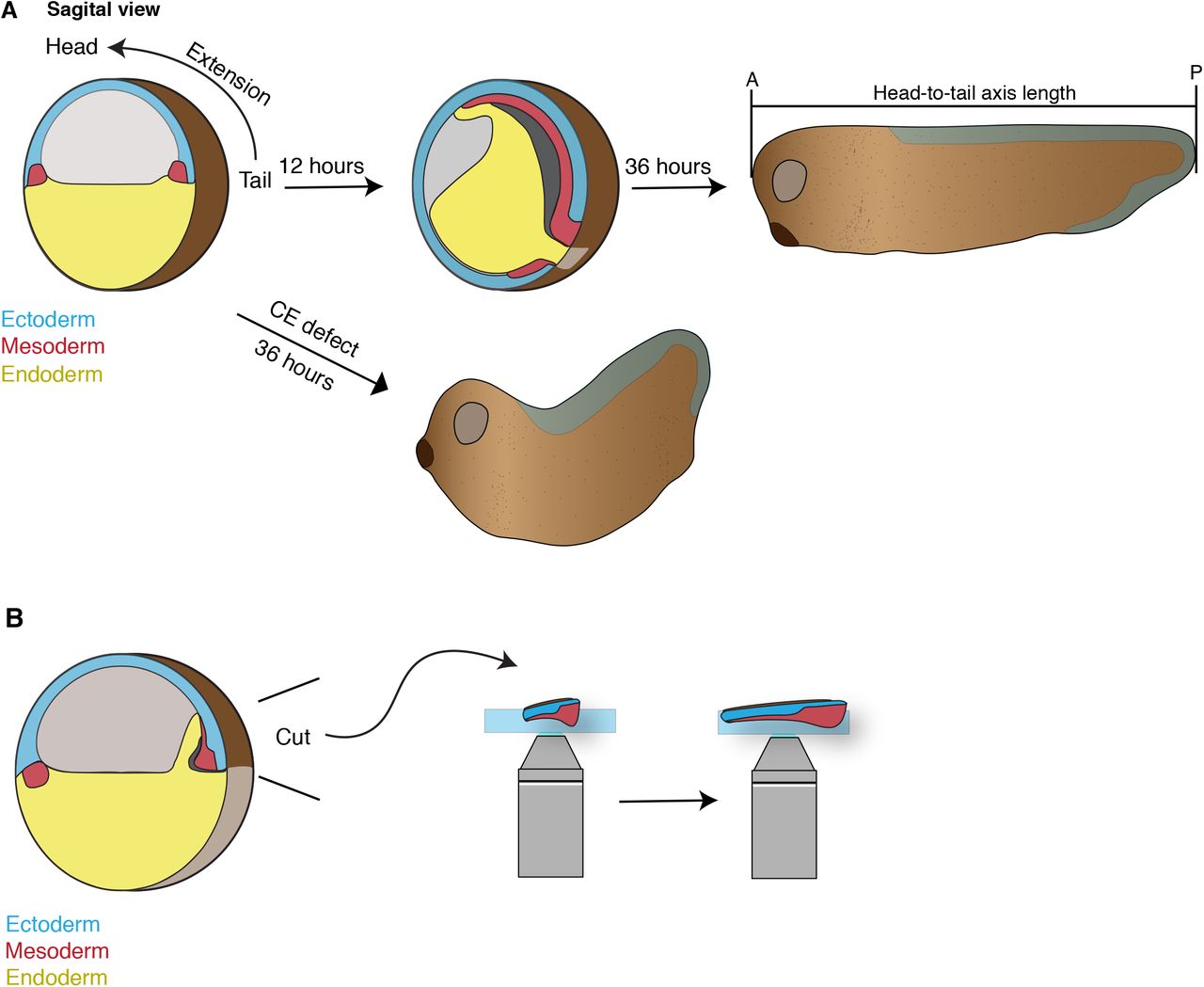
A. Cartoon depiction of Xenopus gastrulation, tadpole axis elongation, and the consequence of convergent extension defects. Here the mesoderm in the dorsal marginal zone (DMZ) involutes and undergoes convergent extension to establish the animals anterior-posterior (head-to-tail) axis. This axis will then continue to elongate during tadpole stages. Disruption of CE results in stunted embryos with a classic ‘swayed back’ appearance (lower arrow).
B. Classic embryological techniques were used to excise the DMZ (Keller explant) allowing visualization of CE in real-time.

A. Mean squared displacements (MSD), Δ(t)i, of 10 distinct individual active (red) and passive (blue) vertices. The heterogeneity in individual vertex movements are apparent from the wide variation in individual vertex MSDs. See Theory SI Section 4 for details on the MSD calculation.
B. Schematic showing how vertex mean square displacement was measured relative to yolk particles that are present in the embryonic Xenopus cells. We refer to this as the MSD in the cell frame of reference.
C. Relative mean squared displacement, Δ(t)ret, of vertices with respect to an egg yolk within a cell (cell frame of reference). This eliminates the effect of translational and rotational motion of the entire tissue on active versus passive vertex dynamics.
D. Mean squared displacement of a pair of active and passive vertices in the lab frame of reference.
E. Schematic showing how vertex mean square displacement was measured relative to a neighboring vertex from other cells. This is the MSD in the nearby vertex frame of reference.
F. Relative mean squared displacement, Δ(t)rel, of the same pair of active and passive vertices in D (above) with the displacement analyzed relative to a nearby quasi-stationary vertex.
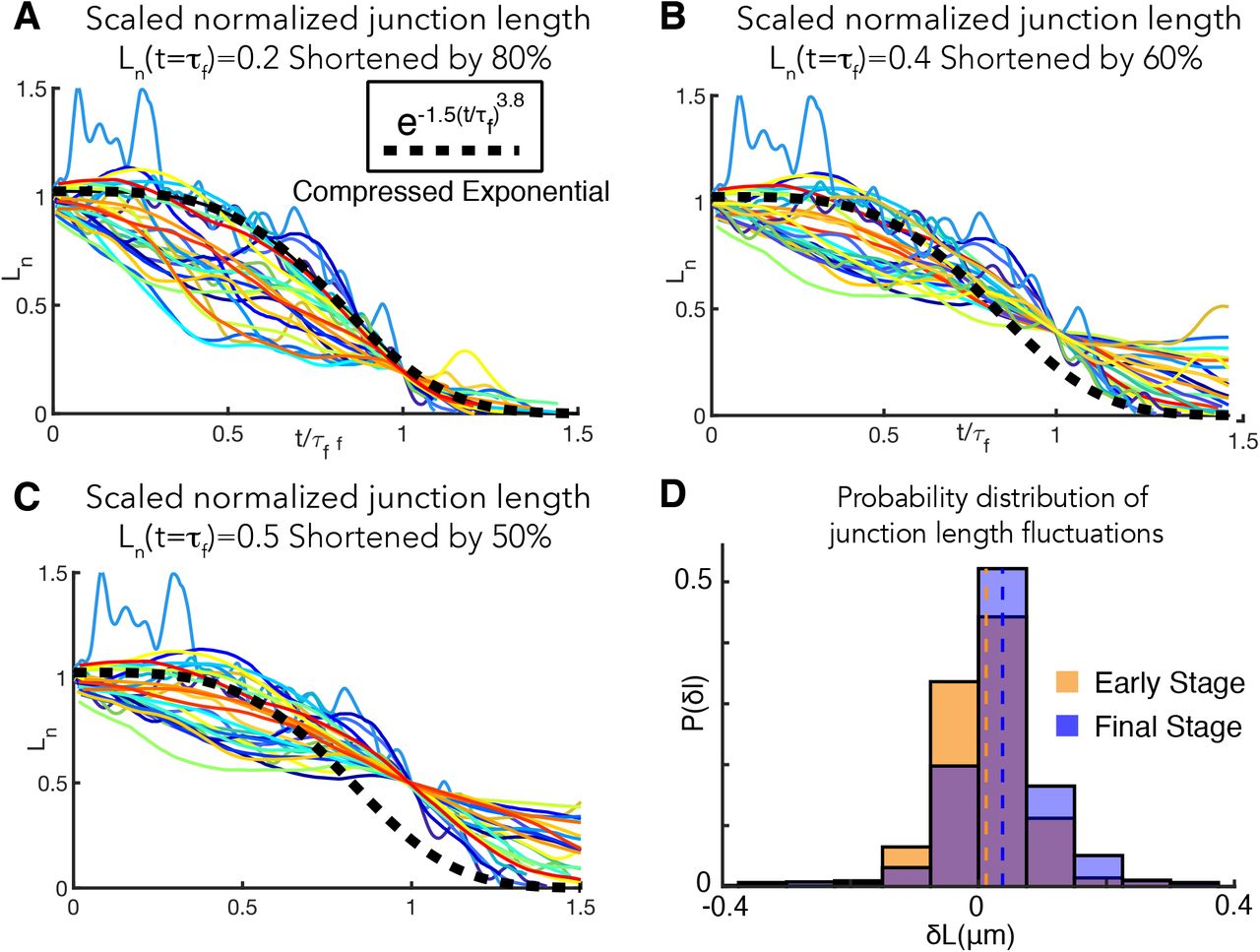
A. The self-similarity of Ln nearly collapsing onto a single universal curve (black dashed line; compressed exponential) when the time axis is scaled by the relaxation time τf is robust to alternative definition of the relaxation time. When the relaxation time is defined as Ln(t = τf) = 0.2, the underlying self-similarity of the cell rearrangement process contributing to CE is evident.
B. When the relaxation time is defined as Ln(t = τy) = 0.4, the underlying self-similarity of the cell junction length change contributing to CE begins to deviate from the compressed exponential.
C. When the relaxation time is defined as Ln(t = τy) = 0.5, the underlying self-similarity of the cell junction length change contributing to CE deviates from the compressed exponential.
D. To identify the trend in increasing persistence of junction shortening, the probability distribution of instantaneous junction length fluctuations at earlier (orange) and later (blue) time frames are shown (see SI, Section 3 for the definition of early and late stages). Dashed red and black lines denote the mean junction length change at early and late times respectively. The mean junction length change become more positive at the final stage (i.e. late times) indicating a positive reinforcement effect that enables more persistent junction shortening.

A. Histogram of active (red) and passive (blue) vertex displacements, referred to as the van Hove function (see Eq. (6) in SI Section 4), shows distinct non-Gaussian functional form. Inset shows deviation of the van Hove function from fits to Gaussian function  for the active vertex and
  for the passive vertex. Probability distribution of distances moved over a time scale of δt = 40s, clearly shows the enhanced movement of active vertices as compared to passive vertices. Probability distribution is obtained for 20 individual vertices from 10 embryos.
B. van Hove distribution of active (red) and passive (blue) vertex displacements at δt = 4s. Van Hove distribution for both active and passive vertices are well fit by a Gaussian distribution indicative of normal diffusive movement at short time scales.
C. Average vertex speed distribution for active (red) and passive (blue) vertices at τ = 4s (see SI, Section 4). The speed distribution peaks at low values of average speed and rapidly decays of zero, showing similar trends for both active and passive vertices at τ = 4s.
D. Average vertex speed distribution for active (red) and passive (blue) vertices at τ = 60s. The distribution peaks at intermediate values of average speed. The active vertex speed distribution decays slower for larger values of the average velocity as compared to passive vertices. This is indicative of enhanced movement of active vertices.
E. Velocity autocorrelation function (VACF) for active (red) and passive (blue) vertices at τ = 4s (see SI, Section 4). Active and passive vertex velocity autocorrelation rapidly decay to zero over a time scale of ~5s. Individual vertex correlations are plotted as solid lines. Mean is plotted as dashed lines. Active and vertex velocity correlations are similar in time at a short time interval, τ = 4s.
F. Velocity autocorrelation function (VACF) for active (red) and passive (blue) vertices at τ = 60s (see SI, Section 4). Active vertex velocity is more persistent in time at this longer time interval compared to the passive vertex velocity. VACF quantifies the emergence of persistent motion of the active vertex at τ = 60s. The persistence time of the velocity correlation is over 50s.
G. For non-shortening vertices (magenta, black), the overlap with its initial positions, as quantified by 〈Q (δt)〉 decays slower compared to active vertices (red). The overlap decays to 0 in the time interval probed for active vertices. The decay in the self-overlap parameter for passive vertices are comparable to non-shortening left and right vertices. See Theory SI, Section 5 for further details.
H. The four-point susceptibility, Χ4(τt) = 〈Q(δt)2〉 – 〈Q(δt)〉2, is calculated from the moments of 〈Q(δt)〉. The Χ4(δt) for non-shortening left (black) and right (magenta) vertices do not show a peak in the time frame analyzed. See Theory SI, Section 5 for further details on the calculation of four-point susceptibility.
I. Temporal autocorrelation of the cell-cell contact length fluctuations during junction shortening in experiments and in simulations. Inset shows the mean autocorrelation of junction length fluctuations. It is fit by an exponential function,  , where τL is the persistence time of junction length fluctuations. Error bars are from the standard deviation. See Theory SI, Section 10 for further discussion.
J. Phase diagram for an alternative model (Theory SI, Section 15) of active versus passive vertex contribution to junction shortening. Instead of accelerating vertices, we consider the velocity of vertices to be constant. Active vertex velocity is taken to be larger than the passive vertex. Simulations using the alternative model tell us that the viscoelastic parameter controls junction shortening. Our conclusion on the importance of the viscoelastic parameter in effecting junction shrinking is independent of the details of the vertex dynamics.
K. Ln for shortening junctions from wild type embryos in comparison to simulations. The expected compressed exponential function form is in red.

A. Immunostaining for endogenous Cdh3 showing that the endogenous protein forms cadherin cis-clusters.
B. An alternative definition of cluster size was used to analyze differences in cadherin clustering (see Theory SI, Section 8). By fitting an exponential function to the spatial autocorrelation of cadherin intensity fluctuation, we extract the characteristic cadherin cluster size. Violin plot shows the Cdh3 cluster sizes for active versus passive vertices in shortening junctions. 1538 frames from 10 embryos were analyzed. t-test shows significant differences between Cdh3 clustering near active versus passive vertices (p=0.02).
C. Violin plot of Cdh3 cluster sizes for left versus right vertices in non-shortening junctions. 2062 frames from 7 embryos were analyzed. t-test did not indicate significant differences between Cdh3 clustering near left versus right vertices (p=0.13).

A. Embryos were injected with Cdh3-MO and membrane-BFP in a single dorsal blastomere at the 4-cell stage resulting in mosaic depletion of Cdh3. Here immuno-staining for Cdh3 shows that the protein was depleted specifically in cells that received the morpholino, as marked by membrane-BFP.
B. Cdh3 immuno-staining intensity was measured in control cells and neighboring Cdh3-MO cells from mosaic animals. These data were derived from three replicate experiments and statistically analyzed by t-test.
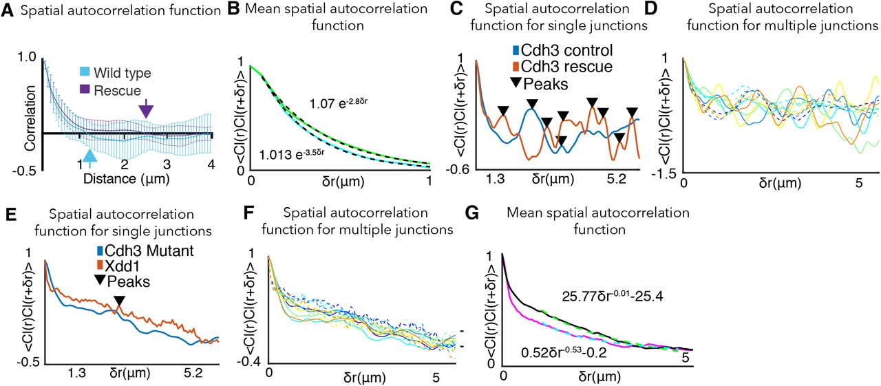
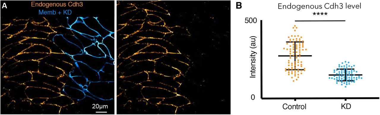
A. Spatial autocorrelation of Cdh3 intensity fluctuations for wild type (60 frames, obtained from 10 embryos) and Cdh3-rescue (58 frames, obtained from 4 embryos). The characteristic correlation length decays to zero at ~1 μm, for both wild type and rescue embryos. Error bar is the standard deviation.
B. Mean spatial autocorrelation of Cdh3 intensity fluctuations for wild type and rescue with functional fits to the decay behavior. Both spatial correlations can be fit to an exponential. This is evidence for a characteristic spatial scale for the correlation in spatial Cdh3 intensity fluctuations.
C. Single junction spatial autocorrelation of cadherin intensity fluctuations in Cdh3 wild type and rescue embryos. Local maxima in the Cdh3 spatial correlation are indicated as peaks (see SI, Section 17). This shows the well-defined spatial periodicity in Cdh3 distribution along the cell-cell junction for both wild type and rescue embryos.
D. Spatial autocorrelation of cadherin intensity fluctuations in Cdh3 control (solid lines) and Cdh3 rescue (dashed lines) embryos along a single junction at 5 different time frames.
E. Single junction spatial autocorrelation of cadherin intensity fluctuations in Cdh3 mutant and Xdd1 mutant embryos. As compared to wild type and rescue embryos, local maxima in the Cdh3 spatial correlation is highly suppressed. The spatial periodicity of Cdh3 distribution along the cell-cell junction is not seen.
F. Spatial autocorrelation of cadherin intensity fluctuations in Cdh3 mutant (solid lines) and Xdd1 mutant (dashed lines) embryos along a single junction at 5 different time frames.
G. Mean spatial autocorrelation of Cdh3 intensity fluctuations for Xdd1(black) and Cdh3 mutant (magenta) with functional fits to the decay behavior. Both spatial correlations decay to zero is better fit to a power law. This is evidence for the lack of characteristic spatial scale for the correlation in spatial Cdh3 intensity fluctuations.
Acknowledgements
We thank Dan Dickinson for use of the iSIM microscope and for critical reading and helpful discussions. This work was supported by grants from the NICHD (R21HD084072) and the NIGMS (R01GM104853) to J.B.W. and from the N.S.F. (Phys 17-08128) and the Collie-Welch Chair through the Welch Foundation (F-0059)
References
Theory Supplement References


