

Summary
Animals must adapt their behavior to survive in a changing environment. Behavioral adaptations can be evoked by two mechanisms: feedback control and internal-model-based control. Feedback controllers compare current with desired sensory state and generate motor output to minimize this difference. In contrast, internal models use previous sensory-motor history to update parameters required for predictive motor control. In this study we use multiple perturbations in visual feedback to show that larval zebrafish acutely adapt their swimming behavior depending on the feedback received while swimming. These short-term changes do not affect an initial stereotyped ballistic portion of the swimming event and are unaffected by the ablation of cerebellar Purkinje cells. Contrarily, consistent long-term changes induce larvae to gradually change their behavior, including the ballistic period kinematics, in a cerebellar-dependent process. We conclude that swimming in larval zebrafish can be understood as a feedback control system that is recalibrated by cerebellar output.
Highlights
Larval zebrafish acutely adapt their ongoing behavior to changed visual reafference
This acute motor adaptation is likely to be implemented by a feedback controller
Persistent change in reafference modifies the parameters of this controller
The cerebellum is required for this recalibration
Introduction
The interaction between animals and their surroundings changes constantly, due to changes in the environment or processes such as development, growth or injury, which modify the body plant of the animal. Nevertheless, precise behavior is so important that evolution has provided animals with mechanisms to adapt their behavior in these changing conditions.
Many stimulus-driven behaviors result in the effective cancellation of the stimulus that evoked them. Examples include the optokinetic reflex (Cohen, 2011), in which retinal slip drives eye motion that will set this slip to zero. If the stimulus is monitored constantly, a feedback control loop with well-tuned parameters may provide an appropriate mechanism for performing the task of setting the stimulus to zero (Ohyama et al., 2003). This happens online, so feedback controllers are limited by the time delay required for sensory processing, which in the case of visual feedback is estimated to be between 100 to 300 ms (Barnett-Cowan and Harris, 2009; Brenner and Smeets, 2003; Desmurget and Grafton, 2000; Saunders and Knill, 2003, 2005). If the processing of sensory information is long with respect to the duration of the motor action, the current state of the body will change dramatically by the time the feedback signal starts to influence the motor command, and will therefore implement an inappropriate correction based on out-of-date sensory feedback. In addition, feedback controllers require the measurement of the quantity they are trying to control. Direct sensors for these do not always exist so these quantities need to be inferred, and even when they do exist, these sensors are vulnerable to neuronal noise.
To overcome these limitations of feedback motor control, the brain can encode internal models of different parts of the body and the effect of motor activity on sensory input. These can be trained by previous sensorimotor history to modify the behavior in a predictive manner (Kawato, 1990; Kawato et al., 1987; Wolpert et al., 1995). These models monitor the sensorimotor transformation performed by a motor plant and are able to learn a forward or an inverse function of this transformation either to predict sensory consequences of a motor command or to provide an appropriate feedforward command to reach a desired sensory state. It is widely believed that internal models exist in the central nervous system and that in vertebrates, the cerebellum plays a major role in encoding them (Lisberger, 2009; Nowak et al., 2007; Wolpert et al., 1998). This is supported by multiple loss-of-function studies that have demonstrated that intact cerebellar activity is required for predictive motor control (Izawa et al., 2012; Miall et al., 2007; Yavari et al., 2016).
In this study, we investigate the interplay between feedback controllers and internal models and the role that the vertebrate cerebellum plays in updating them. In order to do this, we make use of the larval zebrafish optomotor response (OMR) (Fleisch and Neuhauss, 2006), a behavior shared by many animals (Götz, 1968; Shi et al., 2018) by which they turn and move in the direction of perceived visual motion. As larvae, zebrafish swim by performing bouts that comprise several full tail oscillations and last around 350 ms. Spontaneously, bouts are typically elicited at a frequency of about 1 Hz and are separated by quiescent periods called interbouts (Budick and O’Malley, 2000). Previous work has shown that larval zebrafish are able to adapt their optomotor behavior within a bout depending on the magnitude of reafferent sensory feedback that they receive upon swimming in a closed-loop experimental assay (Ahrens et al., 2012; Mu et al., 2019; Portugues and Engert, 2011).
Here we extend this virtual reality setup to introduce additional perturbations in sensory feedback that include time delays and gain changes, to demonstrate that larval zebrafish adapt to unexpected changes in sensory feedback with a delay that lasts ~ 220 ms. Behavior during this initial portion of the bout is ballistic in a sense that it is independent of current sensory feedback. Such delayed reaction suggests that this adaptive behavior is implemented by a feedback controller as opposed to an internal model-based mechanism. To support this, we show that behavioral adaptation to unexpected changes in sensory feedback does not require an intact cerebellum. However, when the interaction between swimming and the sensory feedback is changed consistently over several hours so that this new interaction can be learned and predicted, the cerebellum can implement long-term changes in optomotor behavior, including modifications in the initial ballistic portion of the bout.
These results suggest that adaptive locomotion can be understood as a feedback control mechanism whose parameters can be modified by the cerebellum. The feedback controller implements fast behavioral adaptations to unexpected changes in the environment, whilst the cerebellar internal model calibrates this controller according to consistent and predictable environmental features. We use modeling and whole-brain functional imaging to show that the neuronal requirements for this mechanism do indeed exist in the larval zebrafish brain.
Results
Perturbations in visual reafference during a bout result in acute behavioral adaptation with a 220 ms delay
When an animal, such as larval zebrafish, moves in its visual environment in a given direction, it naturally experiences optic flow in the opposite direction (Figure 1A, B). We will refer to the velocity of the optic flow elicited by swimming of a zebrafish larva as visual reafference (Figure 1B). To investigate how perturbations in visual reafference affect ongoing swimming behavior, one needs to have experimental control over the rules that determine how motor behavior translates to sensory reafference in order to manipulate these rules and observe resulting behavioral changes. To this end, we took advantage of a closed-loop experimental assay (Ahrens et al., 2012; Portugues and Engert, 2011), as shown in Figure 1C. Briefly, in this assay, a head-restrained larva was able to swim in response to a forward moving grating, a behavior known as the OMR. A high-speed camera captured this behavior, and parameters of the tail movements were used to estimate the velocity that the fish would have reached if it were freely swimming. To provide the larva with visual reafference, this estimated velocity was then subtracted from the initial stimulus velocity such that the larva experienced the sensory consequences of its own swimming (Figure 1C, D; see Closed-loop experimental assay in head-restrained preparations in Methods for further details).

(A) When a larval zebrafish swims forward with respect to the visual environment (left), the environment moves backwards with respect to the fish (right). Black-and-white grating depicts visual environment of the fish. Green color denotes variables expressed in motor coordinates, such as tail movement and resulting position or velocity of the swimming larva. Magenta color denotes variables expressed in sensory (visual) coordinates, such as observed position or velocity of the visual environment. This color-code is used throughout the paper.
(B) Change in position and velocity of the swimming fish with respect to the visual environment (left) and of the environment with respect to the fish (right) during tail movement. In all figures, decrease of environment position and velocity along the y-axis means that fish moves forward with respect to the environment. In (B), (D) and (E), vertical shaded bars indicate swimming bouts. In this paper, decrease of environment velocity elicited by swimming is referred to as visual reafference.
(C) Behavioral rig (left) and the closed-loop experimental assay (right) used to induce OMR and to study its adaptation to perturbations in visual reafference. A forward moving grating (exafferent sensory stimulus) was presented to a head-fixed larva with a projector (direction of the grating motion is indicated with magenta arrows), and tail movements of the fish were monitored with a camera. In the closed-loop assay, swimming of the larva results in deceleration of the grating, indicated by a magenta arrow pointing downwards (see Closed-loop experimental assay in head-restrained preparations in Methods for details). This panel is modified from (Portugues and Engert, 2011)). Scale bar is 1 mm.
(D) Raw data traces recorded during one experimental trial. Forward motion of the grating elicited tail movements (OMR) that were used to estimate forward velocity of the fish. This estimated velocity was subtracted from the exafferent sensory stimulus to provide larvae with visual reafference. In this example trial, reafference condition was set to normal for simplicity.
(E) Schematic representation of all reafference conditions used in this study: (Ei) gains of the closed-loop; (Eii) shunted and non-shunted lags of the reafference; (Eiii) gain drops (see Closed-loop experimental assay in head-restrained preparations in Methods for details). Vertical blue and red bars indicate normal reafference and open-loop conditions, respectively. Red triangles indicate that in both shunted and non-shunted lag settings, reafference is insufficient in the beginning of the bout compared to the normal reafference condition, blue triangle indicate that only in the non-shunted setting, reafference is excessive after the end of the bout.
As mentioned above, in the closed-loop assay, the way in which the behavior translates to changes in the visual stimulus is under experimental control. During our experiments, we used perturbations in reafference that fall into three distinct conditions designed to probe the space of possible behavioral adaptation (Figure 1E). The first reafference condition, which has been previously used in the literature (Ahrens et al., 2012; Portugues and Engert, 2011), we call gain change and this corresponds to changing the gain of the experimental closed-loop, such that larvae receive more or less visual reafference when they swim (Figure 1Ei). Note that a gain of 0 corresponds to open-loop and a gain of 1 to freely-swimming conditions (respectively, red and blue vertical bars in Figure 1E). The second condition we call lag, and this corresponds to introducing an artificial temporal delay between the behavior of the larva and the reafference it experiences (Figure 1Eii). In the shunted lag version of this condition, the reafference is automatically set to zero when the larvae stop swimming (Figure 1Eii, bottom). The lag conditions test the temporal relationship between the behavior and its related reafference. The final reafference condition we term gain drop, and this corresponds to dividing the first 300 ms of a bout into four 75-ms segments and setting the gain during one or more of these segments to zero (Figure 1Eiii). Different gain drop conditions are labeled by four numbers that are either 1 or 0, depending on the gain of that particular bout segment. The condition 1100 for example, had normal reafference during the first 150 ms of the bout but no reafference for the next 150 ms. After 300 ms, the reafference is always normal. These gain drop conditions test whether perturbations in reafference lead to same behavioral adaptations regardless of when they occur within the bout.
In a first set of experiments, we set out to determine the acute behavioral changes in response to the perturbations in reafference described above. By acute, we refer to changes in a bout in response to a perturbation in reafference during that same bout. Individual wild-type larvae were exposed to 15-second trials during which a grating moved in a caudal to rostral direction at 10 mm/s. Larvae responded by performing swimming bouts and the reafference conditions were randomized in a bout-by-bout basis (Figure 2A). The results for the mean bout and interbout duration are presented in Figure 2B-D.

(A) Protocol of acute OMR adaptation experiment. It included four phases: calibration phase, pre-adaptation phase, acute adaptation phase, and post-adaptation phase. Reafference conditions were randomized in a bout-by-bout basis during the acute adaptation phase, and were set to normal during other phases (see Acute adaptation experimental protocol in Methods for further details). Data presented in subsequent panels were acquired during the acute adaptation phase.
(B-D) Mean bout duration (top, i) and interbout duration (bottom, ii) as a function of reafference condition. Each dot in (B-D) and each colored line in (E) represents data averaged across all bouts within one reafference condition in one larva, and then across larvae; vertical lines in (B-D) denote SEM across larvae; n = 100. Gray triangles in (D) indicate two gain drop conditions, where in both cases the gain was set to 0 during the same number of 75-ms segments of a bout but the behavior was adapted differently depending on what bout segment had a perturbed reafference. See more details in the text.
(E) Bout power profile as a function of reafference condition. Dark and light gray areas indicate ballistic and reactive bout periods, respectively. Blue triangles indicate that if perturbation in reafference was introduced once the bout had already started (as in gain drop condition with gain profiles 1000, 1100), the deviation in the respective mean bout power was observed only around 220 ms after the start of the perturbation. See more details in the text.
For the three types of reafference conditions, mean bout durations (Figure 2Bi-Di) increased when the overall reafference presented was less than normal (gain 1). This was particularly noticeable for the very low gains 0 and 0.33 (Figure 2Bi), under lag and shunted lag conditions (Figure 2Ci) and under gain drop conditions where more than one bout segment had gain 0 (Figure 2Di). Interestingly, the observed increase in bout duration was close to linear as a function of the lag and, as expected, it did not show a significant difference between the lag and shunted lag cases (compare black and gray dots in Figure 2Ci), as these two conditions only differed in whether the speed of the forward moving grating returned to baseline upon termination of the swimming bout (shunted lag) or not (lag) (Figure 1Eii). A result worth noting is that under the gain drop condition, the mean bout duration was differentially prolonged depending on what bout segment had a perturbed reafference. Overall, a segment with a gain of 0 had a larger effect on increasing the bout duration the earlier it occurred within the bout: compare for example the cases for gain profiles 0111 and 1110 (gray triangles in Figure 2Di).
The results in interbout duration are displayed in Figure 2Bii-Dii. Decreasing the gain to values below 1 initially resulted in shorter interbouts (gain 0.66) although further decreases reversed this tendency to the extent that in the current experimental paradigm, interbouts at gain 0 were longer than those at gain 1 (Figure 2Bii), in contrast with (Portugues and Engert, 2011). It is interesting to note that for gains below 0.5, the larva’s velocity was less than 10 mm/s (Figure 1Ei) so it could not reverse the direction of the forward moving grating when it performed a bout. Further experiments are required to elucidate whether this fact underlies the observed reversed trend in interbout duration. Under the lag conditions, mean interbout duration increased with longer lag only in the non-shunted setting, whereas if the reafference was shunted upon termination of the bout, the mean interbout duration became independent of the lag (compare black and gray dots in Figure 2Cii). This demonstrates that the duration of a bout and a subsequent interbout can be independently influenced by the reafference. Explicitly, insufficient reafference in the beginning of the bout, something that is present in both non-shunted and shunted lag settings (red triangles in Figure 1Eii), results in an increase of bout duration (Figure 2Ci), whereas excessive reafference after the end of the bout, something that is only present in a non-shunted lag setting (blue triangle in Figure 1Eii), lengthens the interbouts. The results for interbout duration under the gain drop condition showed a decrease in interbout duration following a bout with gain drop. In contrast with the results for mean bout duration (Figure 2Di), interbouts were affected more when the gain was dropped in segments closer to the end of the bout: compare for example the cases for gain profiles 0001 and 1000 (gray triangles in Figure 2Dii).
In order to identify the time it takes larval zebrafish to process visual feedback, we analyzed the temporal dynamics of the tail beat amplitude within individual bouts in the form of bout power (Figure 2E; see Behavioral data analysis in Methods for details). Comparing the mean bout power profiles across different reafference conditions revealed that if the reafference was different from that of gain 1 from the very beginning of a bout (as in gain change, lag and shunted lag conditions), the mean bout power profile started to deviate only 220 ms after the bout onset (Figure 2Ei, 2Eiii, 2Eiv). However, if the change in the reafference was introduced once the bout had already started (as in the gain drop condition with gain profiles 1000, 1100), the deviation in the respective mean bout power was observed only around 220 ms after the start of the perturbation in reafference (see blue traces on Figure 2Eii, indicated by blue triangles). This analysis revealed that larval zebrafish are able to implement behavioral changes in response to visual reafference with a 220 ms delay.
This reaction delay prompted us to divide all bouts into two well defined periods: an initial stereotyped ballistic period lasting 220 ms and a subsequent reactive period. A change in reafference condition (regardless of whether this change occurs during the ballistic or the reactive period), can only affect the bout power during the reactive period (Figure S1).
In summary, the results presented in Figure 2 demonstrate that larval zebrafish can change their behavior during optomotor swimming within a bout depending not only on the absolute amount of reafference that they receive, but also on the temporal relationship between their swimming and its accompanying reafference. A close analysis of bout power reveals that it takes larvae 220 ms to implement any behavioral change, which must encompass delays in sensory processing and implementation of behavioral modifications. This observation allows us to define an initial ballistic period of the bout that is stereotyped across reafference conditions and a reactive period during which visual reafference can acutely drive behavioral adaptations. Since the bout power during the ballistic period does not depend on the reafference, it can be used as a readout of the state of the neuronal controller that determines how forward motion of the grating is transformed into optomotor behavior.
Acute adaptation of the OMR to perturbed reafference is not cerebellum-dependent
Many forms of motor adaptation and learning have been show in both zebrafish (Ahrens et al., 2012; Aizenberg and Schuman, 2011; Harmon et al., 2017) and other vertebrates (Ito, 1982; Raymond et al., 1996; de Zeeuw et al., 1989) to involve cerebellar circuitry. We therefore aimed to test the involvement of the cerebellum in the acute OMR adaptation presented in Figure 2. To this end, we generated a transgenic line Tg(PC:epNtr-tagRFP) expressing nitroreductase in all Purkinje cells (PCs) in the cerebellum (see Targeted pharmaco-genetic ablation of PCs in Methods for details). Treatment of PC:epNtr-tagRFP-positive larvae with metronidazole resulted in severe damage of PCs including swelling and destruction of the PC nuclei and aggregation of the neuropil into puncta with complete loss of the characteristic filiform structure (Figure S2). We tested these PC-ablated larvae in the acute adaptation paradigm depicted in Figure 2A.
After PC ablation, zebrafish larvae were still able both to perform the OMR and to adapt acutely to all reafference perturbations (Figure 3). This demonstrates that the acute OMR adaptation described in Figure 2 is not cerebellum-dependent.
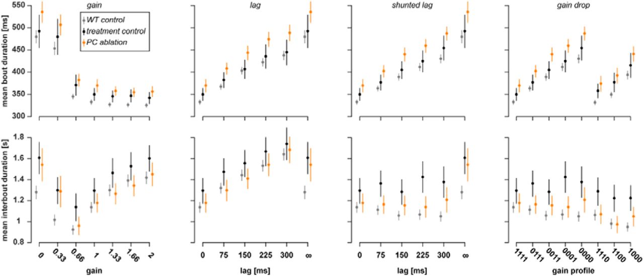
Mean bout duration (top row) and interbout duration (bottom row) in wild-type control group (gray dots, data repeated from Figure 2B-D, n = 100), treatment control group (PC:epNtr-tagRFP−/− larvae, black dots, n = 28), and PC ablation group (PC:epNtr-tagRFP+/−, orange dots, n = 39) as a function of reafference condition. Dots represents data averaged across all bouts within one reafference condition in one larva, and then across larvae; vertical lines denote SEM across larvae. Note that PC-ablated animals demonstrated acute OMR adaptation to perturbed visual reafference similarly to the control groups.
Interestingly, PC-ablated animals displayed increased motor activity: a longer mean bout duration than both treatment controls and wild-types in every single condition and shorter interbouts than the treatment controls. We were reassured by this observed consistent behavioral effect as it confirms the effectiveness of the ablation protocol.
Larval zebrafish can recalibrate the neuronal controller of the OMR
After concluding that the mechanism of acute OMR adaptation is not cerebellum-dependent, we aimed to determine whether larvae could perform long-term motor adaptation and to assess the role of the cerebellum in this adaptive behavior.
To this end, we exposed the animals to a persistent long-term perturbation in reafference, namely to 225 ms lag of the reafference. In contrast to the acute adaptation experimental paradigm, where reafference conditions are randomized in a bout-by-bout basis (Figure 2A), the persistent exposure to the same perturbation in reafference allows animals to learn and predict the new rules of behavior-to-environment interaction. Analysis of trial-to-trial changes in first bout duration during the long-term adaptation experiment is presented in Figure 4A. As expected from previous results (Figure 2Ci), animals adapted to delayed reafference by increasing the bout duration (gray arrows in Figure 4A, B). However, the first bout duration gradually decreased throughout the adaptation session and reached the pre-adaptation level by the end of the session (orange arrows in Figure 4A, C). In addition, when normal reafference was reinstated after the long-term adaptation session, the lag-trained animals demonstrated a significant after-effect of decreased bout duration compared to the animals that were presented with normal reafference through the adaptation session (blue arrows in Figure 4A, D). These results demonstrate that exposure to lag reafference condition for a prolonged time leads to the long-term recalibration of bout duration.

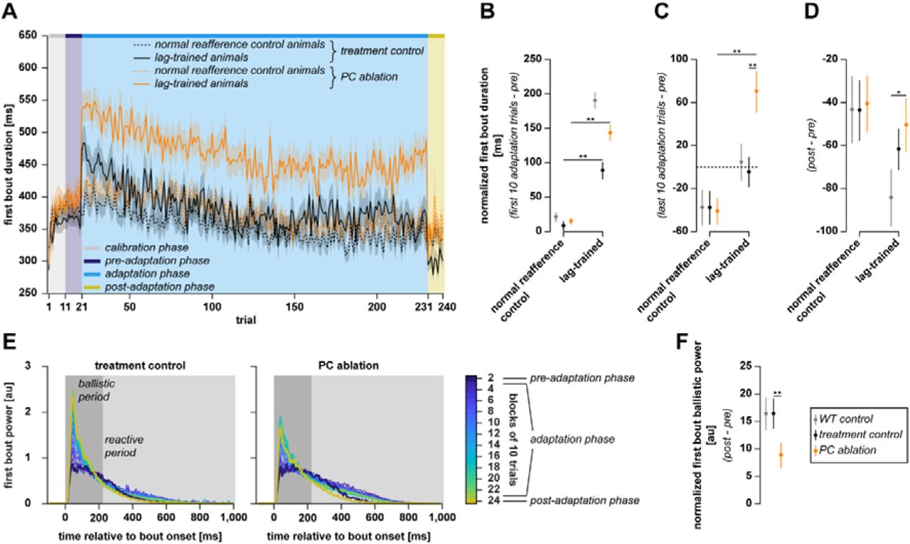
(A) Trial-to-trial changes in first bout duration in normal reafference control animals (dotted broken line, n = 103 larvae) and in lag-trained animals (solid broken line, n = 100 larvae) during long-term OMR adaptation experiment. Black broken lines and gray shaded areas represent mean values and SEM across larvae. Colored areas indicate four phases of the experimental protocol: calibration phase, pre-adaptation phase, adaptation phase and post-adaptation phase. For lag-trained animals, reafference condition was set to 225 ms lag during the adaptation phase and to normal reafference during other phases; for normal reafference control animals, reafference condition was set to normal during the whole experiment. Gray arrow indicates acute OMR adaptation to lagged visual reafference in lag-trained animals (quantified in B). Orange arrow indicates that by the end of the long-term adaptation phase, lag-trained animals decreased their bout duration to the pre-adaptation level even though they were still presented with lagged visual reafference (quantified in C). Blue arrow indicates the after-effect of decreased bout duration observed after the long-term adaptation phase (quantified in D).
(B) Difference between first bout duration during the first 10 trials of the adaptation phase and during the pre-adaptation phase. In (B), (C), (D), and (F), black dots represent data averaged across blocks of 10 trials in one larva and then across larvae; vertical lines denote SEM across larvae. Test used to estimate statistical significance of the observed differences was nonparametric Mann-Whitney U test, with significance level of 5 %, n.s. - p-value > 0.05, * - p-value < 0.05, ** - p-value < 0.01.
(C) Difference between first bout duration during the last 10 trials of the adaptation phase and during the pre-adaptation phase.
(D) Difference between first bout duration during the post-adaptation and the pre-adaptation phases.
(E) Change in mean bout power profiles in normal reafference control animals (left) and in lag-trained animals (right) during long-term OMR adaptation experiment. Colored curves display first bout power profiles averaged across blocks of 10 trials in one larva and then across larvae. Dark and light gray areas indicate ballistic and reactive bout periods, respectively. Red arrows indicate increase of ballistic power during the experiment (quantified in F).
(F) Difference between mean area below bout power curves within ballistic period during the post-adaptation and the pre-adaptation phases.
As reported above, bout power during the ballistic period does not depend on the reafference condition and reflects the state of the neuronal controller that converts sensory information about the moving grating into the OMR behavior (Figure 2E, S11). Therefore, any change in the ballistic power would automatically reflect a change in the controller. Analysis of trial-to-trial changes in first bout power profiles indeed revealed that bout power during the ballistic period gradually increased throughout the experiment (red arrows in Figure 4E, F). This increase did not depend on whether animals were exposed to lag or to normal reafference during the adaptation session (Figure 4F).
We conclude that larval zebrafish are able to recalibrate the parameters of the controller underlying the sensorimotor transformation during optomotor swimming. This recalibration is reflected in three ways. Firstly, there is a decrease of acute adaptation of first bout duration by the end of the long-term adaptation to lag (Figure 4A, C). Secondly, there is an after-effect of decreased first bout duration observed during the post-adaptation phase in lag-trained animals compared to animals presented with normal reafference (Figure 4A, D). Thirdly, there is an increase in first bout power during the ballistic period after the long-term adaptation (Figure 4E, F).
Recalibration of the OMR controller is cerebellum-dependent
After concluding that the parameters of the controller underlying the sensorimotor transformation during the OMR can be modified, we hypothesized that this modification results from updating a cerebellar internal model in response to a consistent long-term perturbation in reafference. To test whether the long-term adaptation is cerebellum-dependent, we conducted the experiments presented in Figure 4 in PC-ablated animals.
Firstly, as expected from the results reported above (Figure 3), we observed that PC-ablated animals acutely adapted to lagged visual reafference by increasing their bout duration (Figure 5A, B). However, in contrast to the control animals, by the end of the adaptation session, lag-trained PC-ablated animals did not decrease their first bout duration to the pre-adaptation level and maintained high motor activity throughout the whole adaptation session (Figure 5A, C). Furthermore, the after-effect of decreased bout duration during the post-adaptation phase in lag-trained animals was also absent after PC-ablation (Figure 5A, D). Finally, the increase in bout power during the ballistic period was also significantly less prominent in PC-ablated animals (Figure 5E, F). Overall, these results demonstrate that the recalibration of the internal OMR controller is cerebellum-dependent.
(A) Trial-to-trial changes in first bout duration during long-term OMR adaptation experiment in four experimental groups: normal reafference treatment control animals (dotted black line, n = 85 larvae), lag-trained treatment control animals (solid black line, n = 85 larvae), normal reafference PC-ablated animals (dotted orange line, n = 83 larvae), and lag-trained PC-ablated animals (solid orange line, n = 90 larvae). Broken lines and shaded areas represent mean values and SEM across larvae. Colored areas indicate four phases of the experimental protocol: calibration phase, pre-adaptation phase, adaptation phase and post-adaptation phase (see legend of Figure 4; see also Long-term adaptation experimental protocol in Methods for further details). Note that lag-trained PC-ablated animals neither demonstrated significant decrease of first bout duration by the end of the long-term adaptation phase (quantified in C), nor the after-effect (quantified in D).
(B) Difference between first bout duration during the first 10 trials of the adaptation phase and during the pre-adaptation phase. In (B), (C), (D), and (F), dots represent data averaged across blocks of 10 trials in one larva and then across larvae; vertical lines denote SEM across larvae. Test used to estimate statistical significance of the observed differences was nonparametric Mann-Whitney U test, with significance level of 5 %, n.s. - p-value > 0.05, * - p-value < 0.05, ** - p-value < 0.01. Gray color represents wild-type control data, repeated from Figure 4.
(C) Difference between first bout duration during the last 10 trials of the adaptation phase and during the pre-adaptation phase.
(D) Difference between first bout duration during the post-adaptation and the pre-adaptation phases.
(E) Change in mean bout power profiles in treatment control animals (left) and in PC-ablated animals (right) during long-term OMR adaptation experiment. Normal reafference control and lag-trained animals were pooled together because no effect of reafference condition on this parameter was observed (Figure 4E, F). Colored curves display first bout power profiles averaged across blocks of 10 trials in one larva and then across larvae. Dark and light gray areas indicate ballistic and reactive bout periods, respectively. Note that in PC-ablated animals, the long-term adaptation effect of increased ballistic power was less prominent than in the treatment control group (quantified in F).
(F) Difference between mean area below bout power curves within ballistic period during the post-adaptation and the pre-adaptation phases.
A feedback controller can drive acute adaptation
After concluding that the internal controller of the OMR can be influenced by cerebellar output, we asked what could be the nature of this controller. One hypothesis that is evident in the literature (Ahrens et al., 2012; Portugues and Engert, 2011), suggests that larval zebrafish acutely adapt OMR to perturbed visual reafference by comparing the observed reafference with an internal representation of expected reafference generated by a forward internal model in the cerebellum. If these two signals are not the same, i.e. if the observed sensory consequences of a swimming bout are unexpected, a resulting performance error signal can influence parameters of ongoing behavior. In the present study, we reported that acute adaptation is not cerebellum-dependent (Figure 3) and that it is only implemented after a relatively long initial ballistic period of 220 ms (Figures 2E, S1). Since delayed adaptation is a prominent feature of feedback control mechanisms, we hypothesized that acute OMR adaptation is implemented by a feedback controller rather than by a forward model-based mechanism. Explicitly, a feedback controller measures a particular variable of a system and generates an output that tries to keep this variable at a set fixed-point value. In the case of the OMR, when fish swim in a closed-loop assay in response to a forward moving grating, the grating slows down with respect to the fish, so it is natural to postulate that fish will swim as long as the visual stimulus is moving forward with respect to them. We therefore defined such a feedback controller and tested its performance in the acute adaptation paradigm presented in Figure 2.
The feedback controller we designed is rather simple (Figure 6A). It consists of three parts: a sensory part, a sensory integration part and a motor output generation part, indicated by the blue, red and green areas in Figure 6A, respectively. The sensory part instantaneously combines the forward and backward grating velocity with independent excitatory and inhibitory weights. This weighted sensory input is then integrated in time by a sensory integrator. The output of the sensory integrator can be interpreted as a forward sensory drive because it increases with longer or faster forward motion of the stimulus, and decreases with backwards motion. This sensory drive is then fed forward to a motor output generator that, whenever it reaches a given threshold, generates a motor output command. As larvae swim in discrete bouts, the model contains a motor integrator that inhibits the motor output generator and eventually leads to the termination of the bout. The output of the motor integrator can be interpreted as a metric of tiredness that ensured that bouts have finite length even when the sensory drive to continue swimming is very high (for example, under an open-loop reafference condition, when fish swims but the grating continues to move forward and the sensory drive continues to accumulate). Finally, to ensure that bouts can last for some time once started in cases when the sensory drive becomes low after bout onset (for example, if the gain of the closed-loop is very high and fish receives a lot of reafference), we introduced a self-excitation loop to the motor output command generator (see Feedback control model of acute adaptation in Methods for further details).
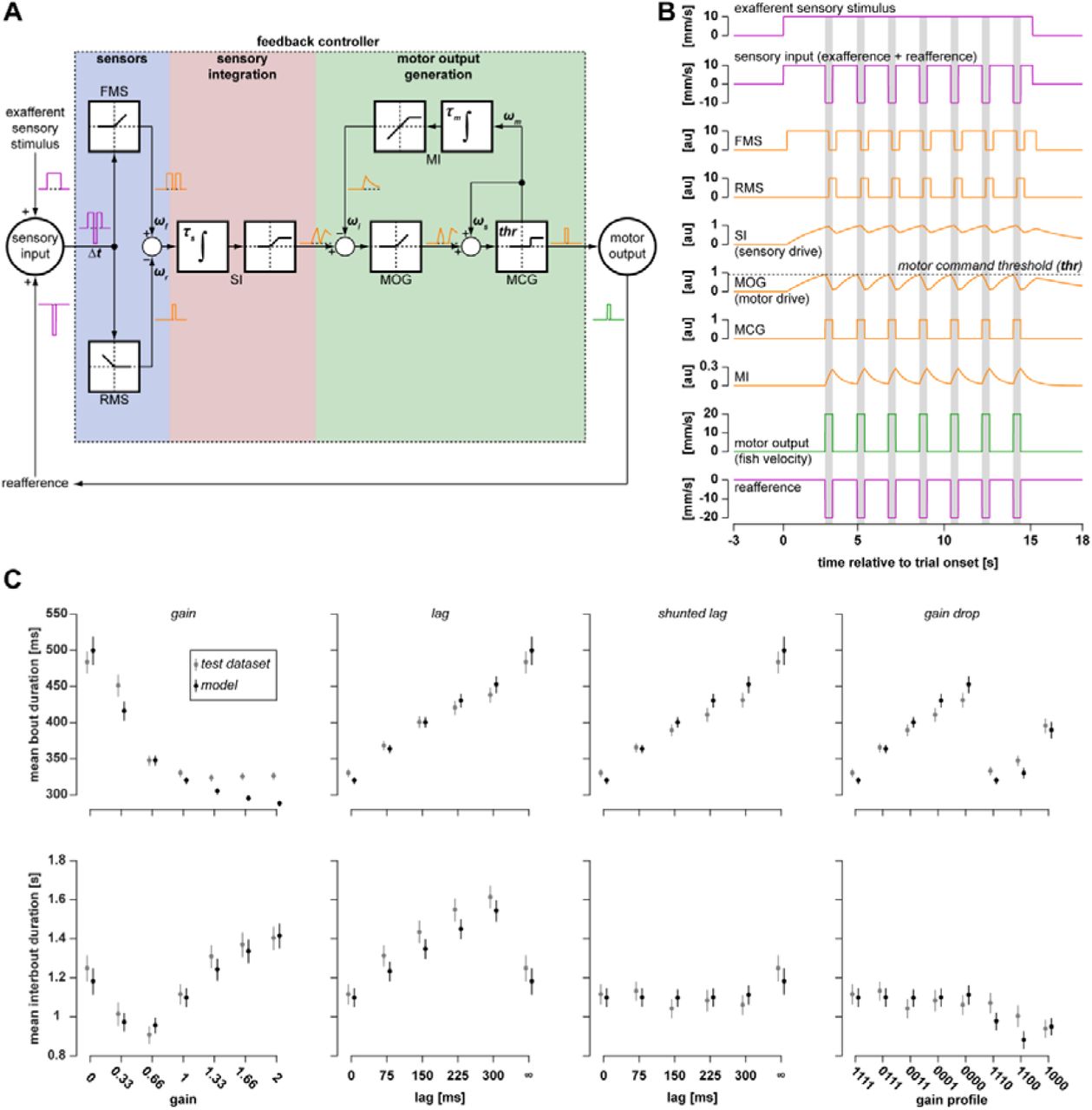
(A) Schematic diagram of the feedback control model. White areas inside the controller depict mathematical operations performed by respective nodes: FMS – forward motion sensor, RMS – reverse motion sensor, SI – sensory integrator, MOG – motor output generator, MCG – motor command generator, MI – motor integrator. Little traces next to connecting arrows depict output of respective nodes in a short one-bout experimental trial. Small Greek letters denote eight parameters of the model. Blue area outlines the sensory part of the controller, red area outlines the part where sensory integration takes place, and green area outlines the motor part of the controller; this color code is preserved in subsequent figures. In (A) and (B), orange lines depict output of the model nodes, magenta and green colors depict variables expressed in sensory and motor coordinates, respectively. See Feedback control model of acute adaptation in Methods for description.
(B) Behavior of the model in an example trial, where reafference condition was set to normal for simplicity.
(C) Acute adaptation of the model to the same perturbations in visual reafference, as presented in Figure 2. Top and bottom rows present, respectively, mean bout and interbout duration as a function of reafference condition. Gray color represent a subset of data shown in Figure 2B-D that was not used for training the model, black color represents output of the model. Dots represent data averaged across all bouts within one reafference condition, and then across subjects (respectively, across larvae or across models fitted to individual larvae); vertical lines denote SEM across subjects; n = 100. Note that the model is able to reproduce acute adaptation to different perturbations in visual reafference presented in Figure 2.
Using cross-validation, we were able to fit the model with a set of parameters such that it generated bouts and interbouts of realistic duration in response to forward moving grating under normal reafference condition (Figure 6B). Furthermore, the behavior of the model under different perturbations in reafference reproduced the main findings presented in Figure 2B-D, including increased motor output in response to decreased or delayed reafference, a difference in adaptation of interbout duration to shunted and non-shunted lags, and different adaptation under the gain drop condition depending on which bout segment had a perturbed reafference (Figure 6C). This allows us to conclude that acute OMR adaptation to perturbed reafference may indeed be implemented by a feedback control mechanism that relies on temporal integration of the sensory evidence and does not necessarily require the generation of expected reafference by a forward model and the computation of performance errors, as was hypothesized previously (Portugues and Engert, 2011).
To test the main assumption of this model, namely, the existence of the sensory integration in the larval zebrafish, and to gain some further insight into the model, we performed whole-brain, light-sheet, functional imaging experiments in head-restrained larvae performing the OMR (Figure 7A).

(A) Light-sheet microscope combined with a behavioral rig used in the functional imaging experiment (see Light-sheet microscopy in Methods for details).
(B) Location of all ROIs that were detected in the imaged brains. Color codes for percentage of larvae with ROIs detected in a given voxel of the larval zebrafish reference brain, showing parts of the brain that were imaged during the experiment. In (B), (F), and (J), presented maps are maximum projections along dorsoventral or lateral axis: ro - rostral direction, l – left, r – right, c – caudal, d – dorsal, v – ventral; fb - forebrain, mb - midbrain, hb – hindbrain; in (B), (F), and (J), scale bars are 100 µm. Note that in rostral and dorsal parts of the midbrain (outlined by dotted black curves), only a few ROIs were detected because these regions were blocked from the scanning laser beams by eye-protecting screens. Colored circles indicate location of example ROIs presented in (C), (D), (G), and (H).
(C) Fluorescence traces of sensory and motor example ROIs in one trial. In (B-F), magenta and green colors represent sensory and motor ROIs, respectively. Vertical gray bars indicate swimming bouts. Note that the sensory ROI responded when the grating started to move forward (indicated by a gray triangle), whereas the motor ROI responded only after the first bout onset (indicated by a black triangle).
(D) Average grating- and bout-triggered fluorescence of example ROIs presented in (C). In (D) and (H), shaded areas indicate SEM across triggers. In (D), (E), (H), and (I), vertical dotted lines indicate respective triggers.
(E) Average grating- and bout-triggered fluorescence of all sensory and motor ROIs pooled from all imaged larvae (n = 6).
(F) Anatomical location of sensory and motor ROIs in the reference brain (see Figure S3 for anatomical reference). In (F) and (J), color codes for percentage of larvae with ROIs of respective functional group in a given voxel of the reference brain.
(G) Fluorescence traces of two sensory ROIs in one trial: one with zero time constant of leaky integration (sensor, blue) and another with time constant greater than zero (integrator, red). Trial where the larva did not perform swimming bouts was chosen to illustrate that the differences in fluorescence rise time are not related to behavior and rather reflect the process of integration. In (G-J) and (B), blue and red colors represent sensors and integrators, respectively.
(H) Average grating-triggered fluorescence of example ROIs presented in (G).
(I) Average grating-triggered fluorescence of all sensory ROIs pooled from all imaged larvae and categorized into sensors and integrators.
(J) Anatomical location of all sensors and integrators in the reference brain (see Figure S3 for anatomical reference).
After segmenting the imaged brains (Figure 7B) into regions of interest (ROIs) (see Functional imaging data analysis in Methods for details), we observed ROIs that increased their fluorescence at the onset of the moving grating (sensory ROIs; see gray triangle in Figure 7C) or when the larvae were performing swimming bouts (motor ROIs; see black triangle in Figure 7C). Analysis of the average fluorescence triggered by grating movement or bout onset (Figure 7D, E) revealed that activity of a large fraction of detected ROIs was either sensory-, or motor-related (respectively, 36 ± 5 % and 40 ± 4 %, mean ± SEM across imaged larvae, n = 6). Motor ROIs were located predominantly in the hindbrain and in the nucleus of the medial longitudinal fasciculus in the midbrain (Severi et al., 2014), and sensory ROIs were mostly present in the hindbrain, midbrain and diencephalic regions, including the inferior olive, dorsal raphe, optic tectum, pretectum, and thalamus (Figure 7F, see also Figure S3 for anatomical reference).
We then focused on sensory ROIs and discovered that the fluorescence rise-time after grating onset varied greatly across these ROIs (Figure 7G-I). To identify whether some of these ROIs integrate sensory evidence in time, we fitted a leaky integrator model to the grating-triggered average fluorescence of each ROI individually. The integration time constant was zero for about a half of sensory ROIs (56 ± 5 %, mean ± SEM across larvae), indicating that these ROIs did not integrate sensory evidence and could be therefore termed “sensors”, as opposed to the remaining 44 ± 5 % sensory ROIs with non-zero time constants which we called “integrators” (Figure 7I). 95 % of the time constants of the integrators fall between 0.1 and 1.3 seconds, with the mean value 0.48 ± 0.15 seconds (mean ± SEM across larvae, data not shown). Sensors and integrators occupied distinct brain regions: sensors were located predominantly in the optic tectum and in the inferior olive, whereas the integrators occupied the dorsal raphe and diencephalic regions (Figure 7J, see also Figure S3 for anatomical reference). The anatomical location of ROIs assigned to all aforementioned functional groups was significantly consistent across all imaged larvae (Figure S4, Movie S5, see also Functional imaging data analysis in Methods for details).
We conclude that certain regions of the larval zebrafish brain (namely the dorsal raphe, pretectum, and thalamus) integrate sensory evidence of the moving grating in time, as shown also in (Bahl and Engert, 2020; Dragomir et al., 2020). This provides an important substrate for the feedback controller-based mechanism of acute OMR adaptation presented in Figure 6.
Discussion
Feedback control mechanism of acute OMR adaptation
In this study, we have shown that larval zebrafish change their behavior within a swimming bout depending on the reafferent visual feedback they receive during that bout, and that these acute, within-bout, changes are not cerebellum-dependent. Furthermore, by using a variety of sensory perturbations, we show that larvae require at least 220 ms to implement these behavioral changes, even if the visual reafference was already altered during the initial 75 ms of the swimming bout. This delay is consistent with previously reported delays involved in processing of feedback visual signals and implementing resulting behavioral adjustments (Barnett-Cowan and Harris, 2009; Brenner and Smeets, 2003; Desmurget and Grafton, 2000; Saunders and Knill, 2003, 2005).
Previous studies proposed that larval zebrafish use cerebellar-dependent forward internal models during acute OMR adaptation (Ahrens et al., 2012; Portugues and Engert, 2011). Forward models can be used to predict the expected sensory consequences of motor actions the animal is about to perform. If the predicted feedback does not match the observed feedback, the behavior needs to be adjusted, and an error signal can be generated to drive changes in the neuronal circuit underlying the OMR.
In contrast, the feedback processing delay and the cerebellar-independence of acute OMR adaptation observed in the present study, suggest that this phenomenon should rather be understood in terms of a feedback control mechanism (Figure 8A). To support this hypothesis, we present a rigid and simple feedback controller that implements the experimentally observed acute behavioral adaptation. The controller is rigid in a sense that it can produce different motor outputs without changing its intrinsic parameters, and simple in a sense that it does not rely on any internal modelling. However, the long-term adaptation experiments demonstrate that under certain conditions, intrinsic parameters of the controller can be changed, and we show that this process does rely on cerebellar output (Figure 8A).

(A) Schematic diagram of the feedback controller that can implement acute OMR adaptation to perturbations in reafference. Cerebellar forward model monitors the efference copies of motor commands and resulting sensory consequences and learns their transfer function. It influences some intrinsic parameters of the controller, presumably, of its motor part. Wavy line denotes the teaching signal used by the forward model to learn the transfer function. The orange arrow denoting the modification of the feedback controller by the cerebellum was drawn towards the premotor circuits to highlight that cerebellar output effectively modifies the final motor output of the controller. It is possible that this modification is achieved through changing parameters in the upstream parts of the OMR circuitry and is mediated by other cerebellar outputs.
(B) Mapping of the crucial functional nodes involved in short- and long-term OMR adaptation onto the larval zebrafish brain. See details in the text.
The sensory part of the proposed feedback controller starts with direction-selective sensors whose output is integrated in time by a sensory integrator. Direction-selectivity can be observed in the brain already at the level of retinal ganglion cells in vertebrates (Barlow and Hill, 1963; Barlow et al., 1964), including zebrafish larvae (Gabriel et al., 2012; Nikolaou et al., 2012). Our whole-brain functional imaging experiments have revealed that the process of sensory integration of the forward visual motion indeed takes place in several brain regions including the pretectum (Figure 7J). Consistent with the architecture of the proposed model, where the sensory integrator receives input from direction-selective sensors, the pretectum receives projections from the contralateral direction-selective retinal ganglion cells (Burrill and Easter, 1994; Gamlin, 2006; Naumann et al., 2016).
An increasing body of work suggests that the pretectum plays a crucial role in whole-field visual processing and visuomotor behaviors in larval zebrafish (Kramer et al., 2019; Kubo et al., 2014; Naumann et al., 2016; Portugues et al., 2014). Naumann et al. (2016) showed that pretectal neurons integrate monocular direction-selective inputs from the two eyes and drive activity in the premotor hindbrain and midbrain areas during optomotor behavior. Our study provides evidence that the pretectum is involved not only in the binocular integration of sensory inputs, but also in temporal integration that underlies the accumulation of sensory evidence (Bahl and Engert, 2020; Dragomir et al., 2020). In essence, we suggest that the output of the pretectum constitutes the sensory drive, which is accumulated over time and is fed to the premotor circuits (Figure 8B).
Long-term cerebellar effects on the feedback controller
Results of the long-term adaptation experiment demonstrate that when the reafference is perturbed consistently over a prolonged period of time in a predictable way, zebrafish larvae gradually adapt their behavior (Figure 4). In contrast with the acute OMR adaptation, these long-term changes are cerebellum-dependent (Figure 5). This suggests that the cerebellum is required to implement this gradual adaptation to a consistent long-term change in reafference and may therefore modify the parameters of the controller underlying the OMR (Figure 8).
The notion that the cerebellum is not involved in online corrections of the movements in response to wrong sensory feedback, but is involved in learning new relations between movements and their feedback in the long-term, is widespread in the cerebellar literature. In two studies (Izawa et al., 2012; Yavari et al., 2016), humans with impaired cerebellar function were able to update the motor program during a reaching task after the feedback of their movements was altered by the experimenters. However, they were not able to update their feedback estimation after the adaptation session, indicating that the cerebellum is involved in acquiring and updating a forward internal model. In our long-term OMR adaptation experiments, a similar process may have taken place. During long-term exposure to consistently perturbed reafference, animals with intact cerebella may have recalibrated their forward models to update their expectations, thus making them match the novel environmental conditions. Since we show that the intrinsic parameters of the OMR controller are under cerebellar control, updating the cerebellar forward model can underlie the modifications in the OMR controller that we observed in the long-term adaptation experiments (Figure 8).
One fact that strongly suggests that the cerebellum in larval zebrafish acts as a forward model during OMR is that, in this study, we observed sensory-related activity in the inferior olive (Figure 7F). The highly sensory nature of PCs’ complex spikes that are known to directly result from action potentials in the inferior olive (Eccles et al., 1966), was also reported recently (Knogler et al., 2019). Inferior olive activity is believed to convey a teaching signal to the PCs (Albus, 1971; Marr, 1969), that updates the internal models in the cerebellum (Imamizu et al., 2003; Kawato et al., 1987) by modifying synaptic weights in the cerebellar circuitry (Ito et al., 1982; Tabata and Kano, 2009). Since the teaching signal must be expressed in the same coordinates as the output of the internal model, the sensory nature of the teaching signal suggests that the cerebellar internal model involved in adaptive OMR is forward in nature (Figure 8).
In conclusion, this study demonstrates that if reafferent sensory feedback received by larval zebrafish during locomotion is perturbed in an unexpected way, the resulting acute behavioral corrections do not require an intact cerebellum and are rather implemented by a feedback controller. However, if the relationship between locomotion and its sensory consequences is changed in way that can be learned and predicted, the cerebellum introduces modifications to this controller. Given the advantages of larval zebrafish as a model organism in systems neuroscience, this provides an exciting opportunity for future research on cerebellar internal models and their role in adaptive behaviors.
Author Contributions
D.A.M. and R.P. conceived of the project. D.A.M. performed most of the experiments, analyzed the data, developed the model and created the figures. A.M.K. generated the Tg(PC:epNtr-tagRFP) zebrafish line and ran preliminary gain drop acute adaptation experiments. L.P. and D.A.M. performed the functional imaging experiments. L.P. programed the experimental protocols for functional imaging and pre-processed the functional imaging data. D.A.M. and R.P. wrote the manuscript with help from all authors.
Declaration of Interests
The authors declare no competing interests.
Methods
Experimental Model and Subject Details
Zebrafish husbandry
All experiments were conducted on larval zebrafish (Danio rerio) at 6 - 7 days post-fertilization (dpf) of yet undetermined sex. All animal procedures were performed in accordance with approved protocols set by the Max Planck Society and the Regierung von Oberbayern (TVA 55-2-1-54-2532-82-2016).
Both adult fish and larvae were maintained at 28 °C on a 14/10 hours light/dark cycle, except for larvae that underwent ablation of cerebellar Purkinje cells (PCs) (see Targeted pharmaco-genetic ablation of PCs in Methods below). Adult zebrafish were kept in a zebrafish facility system with constantly recirculating water with a daily 10% water exchange. The system fish water was deionized and adjusted with synthetic salt mixture (Instant Ocean) to 600 µS conductivity, with the pH value adjusted to 7.2 using NaHCO3 buffer solution. The water was filtered over bio-, fine- and carbon filters and UV-treated during recirculation. Adult zebrafish were fed twice a day with a mixture of Artemia and flake feed.
To obtain larvae for experiments, one male and one female (in some cases, three male and three female) adult zebrafish were placed in a mating box in the afternoon and kept there overnight. The embryos were collected in the following morning and placed in an incubator that was set to maintain the above light and temperature conditions (Binder, Germany). Embryos and larvae were kept in 94 mm Petri dishes at a density of 20 animals per dish in Danieau’s buffer solution (58 mM NaCl, 0.7 mM KCl, 0.4 mM MgSO4, 0.6 mM Ca(NO3)2, 5 mM HEPES buffer) until 1 dpf and in fish water from 1 dpf onwards. The water in the dish was changed daily.
Zebrafish strains
Behavioral experiments were conducted using wild-type Tupfel long-fin (TL) zebrafish strain or transgenic Tg(PC:epNtr-tagRFP) line that was used for PC ablation (see Targeted pharmaco-genetic ablation of PCs in Methods below).
Efficiency of PC ablation was evaluated using the progeny of Tg(PC:epNtr-tagRFP) zebrafish outcrossed to fish expressing GCaMP6s in PC nuclei and RFP in PC somata (Tg(Fyn-tagRFP:PC:NLS-GCaMP6s)) (Knogler et al., 2019). This allowed evaluating effects of the ablation protocol not only on the membrane morphology, but also on the morphology of cell nuclei and somata.
These larvae were homozygous for nacre mutation, which introduces a deficiency in mitfa gene that is involved in development of melanophores (Lister et al., 1999). As a result, homozygous nacre mutants lack optically impermeable pigmented spots on the skin, which enables brain imaging without invasive preparations.
Functional imaging experiments were conducted using transgenic zebrafish strain with pan-neuronal expression of GCaMP6s (Tg(elavl3:GCaMP6s)) (Kim et al., 2017), also homozygous for nacre mutation.
A Z-stack of larval zebrafish reference brain used for anatomical registration of the functional imaging data (see Functional imaging data analysis in Methods below for details) was previously acquired in our laboratory by co-registration of 23 confocal z-stacks of zebrafish brains with pan-neuronal expression of GCaMP6f (Tg(elavl3:GCaMP6f)) (Wolf et al., 2017), homozygous for nacre mutation.
Targeted pharmaco-genetic ablation of PCs
To perform targeted ablation of PCs, we employed Ntr/MTZ pharmaco-genetic approach described previously in zebrafish (Curado et al., 2008; Pisharath et al., 2007; Tabor et al., 2014). Briefly, this method is based on generating a transgenic line expressing nitroreductase (Ntr) in a cell population of interest and treating the animals with prodrug metronidazole (MTZ). Ntr converts MTZ into a cytotoxic DNA cross-linking agent leading to death of cells of interest. To this end, we generated a transgenic line that expressed enhanced Ntr (epNtr; (Tabor et al., 2014) under the PC-specific carbonic anhydrase 8 (ca8) enhancer element (Matsui et al., 2014). We cloned epNtr fused to tagRFP (similar to Tabor et al., 2014) downstream to the aforementioned PC-specific enhancer and a basal promoter. We injected this construct, abbreviated as PC:epNtr-tagRFP into nuclei of single cell stage TL embryos heterozygous for nacre mutation, at a final concentration of 20 ng/ul together with 25 ng/ul tol2 mRNA. Larvae showing strong RFP expression in PCs were raised to adulthood as founders and outcrossed to TL fish to gain a stable line.
Ablation-induced changes in behavior were tested using the progeny of a single founder. The embryos obtained from a PC:epNtr-tagRFP+/− fish outcrossed to a TL fish were screened for red fluorescence in the cerebellum at 5 dpf, and 10 RFP-positive (PC:epNtr-tagRFP+/−) and 10 RFP-negative (PC:epNtr-tagRFP−/−) larvae were kept in the same Petri dish to ensure subsequent independent sampling. At 18:00, most of the water in the dish was replaced with 10 mM MTZ solution in fish water, and larvae were incubated in this solution overnight in darkness for 15 hours. The next morning at 9:00, animals were allowed to recover in fresh fish water. The next day, behavior of 7 dpf MTZ-treated larvae was tested in a respective behavioral protocol. After the experiment, the animals were screened for red fluorescence once again to reassess their genotype after mixing positive and negative larvae in one Petri dish. PC:epNtr-tagRFP−/− and PC:epNtr-tagRFP+/− siblings constituted treatment control and PC ablation experimental groups, respectively.
Efficiency of PC ablation protocol was evaluated using larvae obtained from Tg(PC:epNtr-tagRFP) fish outcrossed to Tg(Fyn-tagRFP:PC:NLS-GCaMP6s) fish. These larvae underwent the same ablation protocol, and z-stacks of their cerebella in RFP and GFP channels were acquired under the confocal microscope (LSM 700, Carl Zeiss, Germany) before and after the ablation (at 5 and 7 dpf, respectively).
Method Details
Closed-loop experimental assay in head-restrained preparations
Both behavioral and functional imaging experiments were conducted using head-restrained preparations of 6 or 7 dpf zebrafish larvae, similar to (Portugues and Engert, 2011). For behavioral experiments, each larva was embedded in 1.5 % low melting point agarose (Invitrogen, Thermo Fisher Scientific, USA) in a 35 mm Petri dish. For functional imaging experiments, larvae were embedded in 2.5 % agarose in custom-built plastic chambers, with glass coverslips sealed on the front and left sides of the chamber (with respect to the larva), at the entry points of the frontal and lateral laser excitation beams, and the agarose around the head was removed with a scalpel to avoid scattering of the beams (see Light-sheet microscopy in Methods below). After allowing the agarose to set, the dish/chamber was filled with fish water and the agarose around the tail was removed to enable unrestrained tail movements that were subsequently used as a readout of behavior.
A dish or a chamber with an embedded larva was then placed onto the screen of the custom-built behavioral or functional imaging rig (Figures 1C, 7A, respectively). In the behavioral rig, the screen with the dish was illuminated from below by an infrared (IR) light-emitting diode (LED) (not shown in Figure 1C). A square black-and-white grating with a spatial period of 10 mm was projected onto the screen by a commercial Digital Light Processing (DLP) projector (ASUS, Taiwan). Larvae were imaged through a macro objective (Navitar, USA) and an IR-pass filter with an IR-sensitive camera (Pike, Allied Vision Technology, Germany, or XIMEA, Germany) at 200 frames per second. The functional imaging rig was built in a similar way, with the two differences:
IR LED illuminating the screen with the chamber was directed from above (not shown in Figure 7A) and the image was reflected on a hot mirror to reach a camera (XIMEA, Germany).
DLP projector used to provide visual stimulation (Optoma, USA) was mounted with a red-pass filter to avoid bleed-through of the green component of the visual stimulus in the light collection optics.
Stimulus presentation and tail tracking were controlled by the open-source, integrated system for stimulation, tracking and closed-loop behavioral experiments (Stytra) (Štih et al., 2019). Larvae were presented with grating moving in a caudal to rostral direction at 10 mm/s (Figure 1C, D), as such stimulus reliably triggers swimming behavior, termed the optomotor response (OMR), that consists of series of discrete swimming bouts. Experiments were performed in closed-loop (similar to (Portugues and Engert, 2011)), as described below. Before starting an experiment, two anchor points enclosing the tail were manually selected. The tail between the anchor points was automatically divided into 8 equal segments, and the angle of each segment with respect to the longitudinal reference line was measured by Stytra in real time. The cumulative sum of the segment angles constituted the final tail trace (top green trace in Figure 1D). Sliding standard deviation of the tail trace with a time window of 50 ms was computed in real time, and the resulting parameter was referred to as vigor. Vigor is a parameter that is close to zero when larvae do not move their tail and increases when they do, and can be therefore used to estimate the forward velocity that larvae would have reached if they were freely swimming. To compute estimated fish velocity, the vigor was multiplied by a factor that was optimized during the initial calibration phase of the experiment (see Acute adaptation experimental protocol in Methods below) so that that the median estimated velocity during a typical bout was 20 mm/s (bottom green trace in Figure 1D), that corresponds to a freely swimming condition. Swimming bouts were automatically detected in real time by comparing current estimated fish velocity with a set threshold of 2 mm/s. To provide behaving larvae with visual reafference, the estimated fish velocity was subtracted from the initial grating speed during detected bouts (bottom magenta trace in Figure 1D). As a result, larvae could experience the sensory effects of their own swimming. The initial and actually presented grating speeds, tail trace, vigor, estimated fish velocity, reafference condition (see below), and a binary variable denoting whether the fish was performing a bout or not at each acquisition frame constituted the raw data saved after an experiment (Figure 1D).
Importantly, such closed-loop assay enables the experimenters to control and manipulate the reafference that animals receive when they swim and hence to study how perturbations in reafference affect behavior. The reafference perturbations used in this study can be grouped into three distinct categories (Figure 1E):
The first type of perturbation, which has been previously used in the literature (Ahrens et al., 2012; Portugues and Engert, 2011), is called gain change. In the closed-loop experimental assay, the gain parameter was used as a multiplier that converts the estimated swimming velocity of the larva into presented reafference. Therefore, the gain affected the actual forward velocity of the larva in the virtual environment when it performed a bout. If the gain was set to zero, no tail movement could affect the grating speed, and larvae did not receive any reafference; we will refer to this reafference condition as open-loop. If the gain was 1, the median velocity of the larva during a typical bout was 20 mm/s, and we will refer to this reafference condition as normal reafference. The gain values used in the experiments included 0, 0.33, 0.66, 1, 1.33, 1.66, and 2.
The second type of perturbation was called lag, and this corresponds to delaying the reafference with respect to the bout onset. When the lag was greater than zero, normal visual reafference with gain 1 was presented with a certain delay after the bout had started. The lag values used in the experiments included 0 ms lag (corresponds to the normal reafference condition), 75 ms, 150 ms, 225 ms, 300 ms, and infinite lag (i.e. reafference never arrives after the bout onset, that is equivalent to the open-loop condition). In the shunted lag version of this condition, the gain was set to 0 after termination of the bout.
The third type of perturbation was called gain drop, and this corresponds to dividing the first 300 ms of a bout into four 75-ms segments and setting the gain during one or more of these segments to zero. For example, the gain profile 1100 denotes that the gain during bout segments 3 and 4 (i.e. from 150 ms to 300 ms after the bout onset) was set to zero, and during the rest of the bout, it was set to one. Gain drop conditions used in the experiment included 1111 (normal reafference condition), 0111, 0011, 0001, 0000, 1110, 1100, and 1000.
No combinations of reafference conditions were used, e.g. if the gain was different from 1, the lag was set to 0 ms, or if the lag was greater than 0 ms, the gain was set to 1, and in both cases the gain drop was set to 1111.
Note that reafference conditions listed above and presented in Figure 1E are redundant. For example, the gain drop profile 0011 is exactly the same as 150 ms shunted lag, or gain 0 is exactly the same is infinite lag. Reafference conditions are presented in a redundant way to highlight that infinite lag makes a logical sense at the end of the list of lag conditions, and gain 0 makes a logical sense in the beginning of the gain list. The exact non-redundant list of all reafference conditions (18 conditions in total) is presented below:
normal reafference (gain 1, 0 ms lag, and gain drop 1111);
open-loop (gain 0 or infinite lag);
gains: 0.33, 0.66, 1.33, 1.66, 2 (0 ms lag and gain drop 1111);
lags and shunted lags: 75 ms, 150 ms, 225 ms, 300 ms (gain 1);
gain drops: 1110, 1100, 1000 (0 ms lag).
Acute adaptation experimental protocol
The first aim of this study was to investigate how larval zebrafish acutely adapt their behavior to different reafference conditions. Acute adaptation experimental protocol consisted of 240 trials, each trial included a 15-second presentation of the grating moving in a caudal to rostral direction at 10 mm/s, preceded and followed by 7.5-second periods of the static grating (top magenta trace in Figure 1D). Experimental trials were grouped into four phases (Figure 2A):
Calibration phase (trials 1:10). During this phase, the multiplier defining how vigor is converted into estimated fish velocity was automatically calibrated so that the median velocity during an average swimming bout was 20 mm/s. Reafference condition during this phase was set to normal. This calibration was implemented to minimize fish-to-fish variability in velocity estimation that could potentially result from uncontrolled differences in manipulations during embedding larvae in the agarose and in selecting the tail before the experiments. In addition, during this phase, larvae were able to get used to the experimental environment and bring their swimming behavior to a stable level.
Pre-adaptation phase (trials 11:20). During this phase, reafference condition was set to normal. This phase was used to record the baseline behavior before any perturbations in reafference were introduced.
Adaptation phase (trials 21:230). During this phase, reafference condition for each bout was randomly selected from the list of 18 possible reafference conditions (Figure 1E, see also Closed-loop experimental assay in head-restrained preparations in Methods above).
Post-adaptation phase (trials 231:240). During this phase, reafference condition was the same as during the pre-adaptation phase. This phase was introduced to study how the adaptation affected the baseline behavior.
Long-term adaptation experimental protocol
Another aim was to investigate long-term motor adaptation, when the same reafference condition was presented persistently over a long period of time. Long-term adaptation experimental protocol had a structure similar to the acute adaptation experiments with the only difference that all reafference conditions during the adaptation phase were either normal (normal-reafference control animals), or 225 ms lag (lag-trained animals) (Figure 4A).
Feedback control model of acute adaptation
To test whether acute OMR adaptation can be explained by a mechanism that does not involve computation of expected sensory reafference (i.e. forward internal models) and performance errors, we developed a model that does not perform these computations (Figure 6A, B) and tested its ability to adapt its output to perturbations in reafference (Figure 6C).
The model was developed and tested in MATLAB (MathWorks, USA). The input of the model was current speed of the grating and the previous state of the model, and the output was a binary swimming velocity variable: swim or no swim. For simplicity, we did not set out to model individual tail flicks and approximated the swimming behavior of the zebrafish larvae by a binary motor output that equaled 20 mm/s when the fish was swimming and 0 otherwise. This was possible due to the discrete nature of zebrafish swimming behavior at larval stage. Since in this study, we mainly focused on duration of bouts and interbouts, this simplification did not limit the ability to compare the model behavior with behavior of the real larvae.
To design the model, we used the results of the acute adaptation experiment as a starting point (Figure 2B-E). Thus, since larval zebrafish reacted to changes in visual stimulus with a fixed delay of 220 ms (Figure 2E), the input of the model at a given time point was the grating speed 220 ms before that point. We then assumed that forward motion of the grating should have a positive influence on the motor output, whereas reverse motion should have a negative influence. This assumption was based on the fact that if the grating moved forward during a bout (as under open-loop or low gain conditions), this bout was significantly longer than under normal reafference condition, when the grating moved backwards (compare cases for high and low gains in Figure 2Ei). To implement this notion in the model, the first step was to split the input signal into forward and backward components by positive and negative rectification. This was performed by two respective nodes of the model: forward and reverse motion sensors (FMS and RMS, respectively). Rectified signals were then recombined together with independent positive and negative weights (ωf and ωr, respectively). We then proceeded from the fact that when a larval zebrafish was presented with a forward moving grating, it performed a swimming bout only after a certain latency period (Figure 1D, 7C), suggesting that it integrates sensory evidence of the forward grating motion in time until the level of integration reaches a motor command threshold. We therefore introduced a leaky sensory integrator (SI) that integrated recombined output of the motion sensors with a time constant τs Output of the SI should be interpreted as forward sensory drive to swim forward because it increases with longer or faster forward motion of the stimulus, decreases with backwards motion, and drives activity in the motor part of the controller (see below). Activity of the SI was not allowed to be less than 0 (no sensory drive) or greater than 1 (maximum sensory drive). The sensory drive was then fed forward to the motor output generator (MOG), and this process can be interpreted as translation of the sensory input signal into motor coordinates. Accordingly, activity of the MOG was called motor drive. Whenever the motor drive reached a threshold thr, it activated the motor command generator (MCG), and the output of the model was set to 20 mm/s instead of 0. To ensure that the swimming bouts performed by the model do not last forever, we introduced a leaky motor integrator (MI) that integrated the output of the MCG in time with an input weight ωm and a time constant τm. Output of the MI can be interpreted as a metric of “tiredness” that encapsulates possible reasons for bout termination even when high sensory drive incites to continue swimming. This is the case, for example, under open-loop reafference condition, when the grating moves forward and the sensory drive accumulates even though fish swims and tries to reduce the sensory drive. To implement the inhibitory influence of this “tiredness” on the motor output of the model, the MI inhibited the MOG with a weight ωi, thus reproducing a self-evident fact that the longer a bout had been so far, the sooner it would stop. Activity of the MI was not allowed to be greater than 1 (maximum “tiredness”), and it could not inhibit the MOG below 0 (motor drive could not be negative in the model). Finally, to ensure that bouts can last for some time once started in cases when the sensory drive to continue swimming becomes too low immediately after bout onset (for example, under high gain conditions when larvae receive a lot of reafference), we introduced a self-excitation loop to the MCG with a weight ωs.
Therefore, in total, the model had eight parameters. The input and output of the model, as well as activity of its nodes in an example trial with normal reafference are presented in Figures 3B.
The mathematical equations defining behavior of the model are listed below:

t — current time point, t — 1 — previous time point
In
— input of the model (grating speed, where positive values correspond to motion in a caudal to rostral direction)
Out — output of the model (binary swimming velocity variable)
[x]+ = max(x, 0) — positive rectification of x
[x]7#x2212; = min(x, 0) — negative rectification of x
min(x, 1) — saturation of x at 1
ωf — forward input weight
ωr — reverse input weight
τs — time constant of the sensory integrator
ωi — inhibitory output weight of the motor integrator
ωs — feedforward self - excitation weight of the MCG
thr — threshold of the motor output command
ωm — input weight of the motor integrator
τm — time constant of the motor integrator
To evaluate the ability of the model to acutely adapt to different reafference conditions, its performance was tested in a shorter version of the acute adaptation experimental protocol. The protocol was shortened to save the computation time required for fitting the model. One trial consisted of 300 ms of static grating followed by 9.7 second of the grating moving in a caudal to rostral direction at 10 mm/s. The reafference condition of the first bout was always normal, and the reafference condition of the second bout was chosen from a list of 18 reafference conditions used in the acute adaptation experiment (see Closed-loop experimental assay in head-restrained preparations in Methods above). If the model initiated a third bout, the trial was terminated, and the duration of the second bout and subsequent interbout duration constituted the final output of the model in that trial. If the model did not perform the third bout within 10 s of the trial, the final output values were considered NaN’s. One experiment consisted of 18 trials probing behavior of the model under each reafference condition, hence 18 bout durations and 18 interbout durations constituted the final output arrays of the model.
The model was fitted individually to each larva that participated in the acute adaptation experiment (n = 100) using a custom-written genetic algorithm. To obtain training datasets, we generated 18 arrays of bout durations and 18 arrays of interbout durations for each larva, each array corresponding to one reafference condition. We then randomly selected 50 % of data from each array, and computed their mean values. The remaining 50 % are referred to as test datasets.
The fitting algorithm minimized the L1 norm between the output array of the model and a training dataset, normalized by the training dataset. The fitting resulted in 100 sets of the model parameters, each optimized to fit 1 larva. To present the results, we computed the mean values and SEM of the final output arrays of models across 100 sets of parameters, and of the test datasets across 100 larvae (Figures 6C).
Light-sheet microscopy
To test the main assumption of the proposed feedback control model: the existence of the sensory integration in the larval zebrafish brain, we employed whole-brain calcium imaging using a custom-built light-sheet microscope (Figure 7A).
In the microscope, a beam coming from a 473 nm laser source (modulated laser diodes, Cobolt, Sweden) was split with a dichroic mirror and conveyed to two orthogonal scanning arms. Each scanning arm consisted of a pair of galvanometric mirrors (Sigmann Electronik, Germany) that allowed vertical and horizontal scanning of the beam, a line diffuser (Edmund Optics, USA), a scan lens (Thorlabs, USA), a paper screen to protect the fish eyes from the laser, a tube lens (Thorlabs, USA), and a low numerical aperture objective (Olympus, Japan). The emitted fluorescence was collected through a water immersion objective (Olympus, Japan) mounted on a piezo (Piezosystem Jena, Germany), band-pass filtered (AHF Analysentechnik, Germany), and focused on the camera with a tube lens (Thorlabs, USA). Images were recorded using an Orca Flash v4.0 camera (Hamamatsu Photonics K.K., Japan) with Camera Link.
The piezo, galvanometric mirrors, and camera triggering were controlled by a custom-written Python program. The light-sheet was created by horizontal scanning of the laser beams at 800 Hz. The light-sheet and the collection objective were constantly oscillating along the vertical axis with a saw tooth profile of frequency 1.5 Hz and amplitude of 250 µm. At each oscillation, 35 camera frames were acquired at equally timed intervals, with an exposure time of 5 ms. The resulting volumetric videos had a voxel size of 0.6 x 0.6 x 7 µm, and a sampling rate of 1.5 Hz per volume.
Functional imaging experimental protocol
Functional imaging experimental protocol started with 2 minutes of no visual stimulation (projector presenting a black square) to record spontaneous activity. This was followed by a calibration phase (10 trials), a pre-adaptation phase (10 trials) and an adaptation phase (40 trials), similar to the acute adaptation experimental protocol (see above). In four out of six imaged larvae, the calibration phase was omitted because behavior under the light-sheet setup was less consistent than under purely behavioral rigs, and calibration of the swimming velocity often failed due to insufficient number of bouts performed during this phase. For these larvae, the multiplier defining how vigor converts into estimated swimming velocity was set manually to the value resulting from successful calibration in the other two larvae. During the adaptation phase, reafference condition for each bout was randomly set to either normal or open-loop. In addition, two 350-ms pulses of reverse grating motion (rostral to caudal direction) at 10 mm/s were presented during each static grating period (5 and 10 s after the grating stopped moving). These pulses were introduced to disambiguate activity related to swimming from activity related to reverse motion of the grating that accompanies closed-loop bouts. Responses to reverse grating motion were not analyzed in this study.
Quantification and Statistical Analysis
Behavioral data analysis
Analysis of the behavioral data was performed in MATLAB (MathWorks, USA).
Tail angle trace was z-scored and interpolated together with the grating speed trace to a new time array with a sampling period of 5 ms. For each swimming bout automatically detected by Stytra during the experiment, individual tail flicks were detected. One tail flick was defined as a section of the tail trace between two adjacent local extrema, with the magnitude greater than 0.14 rad and the duration not greater than 100 ms. Automatically detected onsets and offsets of the bouts were then corrected to coincide in time with the beginning of the first tail flick and the end of the last flick, respectively.
Only those bouts that occurred while the grating was moving forward were considered for further analysis. For each bout, its duration and duration of the subsequent interbout was computed. If a bout was the last in a trial, its interbout duration was replaced with a NaN value. All bouts that were shorter than 100 ms, or had a subsequent or preceding interbout shorter than 100 ms were also excluded from the analysis as potential tail tracking artifacts.
If the number of remaining bouts performed by a given larva was less than 540, this animal was excluded from the analysis. Additionally, if there was at least one block of 10 trials without any bouts, the animal was also excluded. The final numbers of animals included in the analysis are listed below:
Acute adaptation experiments: 100 TL larvae (wild-type experimental group), 28 PC:epNtr-tagRFP−/− larvae (treatment control group), and 39 PC:epNtr-tagRFP+/− larvae (PC ablation group);
Long-term adaptation experiments:
normal-reafference control animals: 103 TL larvae, 85 PC:epNtr-tagRFP−/− larvae, and 83 PC:epNtr-tagRFP+/− larvae,
lag-trained animals: 100 TL larvae, 85 PC:epNtr-tagRFP−/− larvae, and 90 PC:epNtr-tagRFP+/− larvae.
To analyze the temporal dynamics of the tail beat amplitude within individual bouts, a parameter termed bout power was computed as described below. A 1.1-second long section of the tail trace was selected for each bout, starting from 100 ms before the onset of that bout. The values of the tail trace after the bout offset were replaced with NaN values to exclude the subsequent bouts that could occur within this time window. Resulting segments of the tail trace were then squared and referred to as bout power. The bout power curves were then divided into ballistic and reactive periods (from 0 to 220 ms after the bout onset and from 220 ms onward, respectively) and the areas below the curves within these two periods were computed.
All behavioral data are presented as mean values ± SEM across larvae. To present the results of acute adaptation experiments, we first measured bout and interbout duration, as well as the bout power profiles and areas below the bout power curves during ballistic and reactive bout periods, for each reafference condition for each larva. These data were then averaged across bouts within one reafference condition in one larva, and then across larvae. To present the results of long-term adaptation experiments, we measured aforementioned parameters only for the first bout in each trial. This was done because we assumed that the first bout should not depend on putative short-term sensory-motor memory accumulated during the trial and should therefore reflect potential long-term changes in the circuitry involved in OMR more clearly than subsequent bouts. To quantify the long-term adaptation effects, we divided all trials of the protocol into blocks of 10 and computed the mean value of respective parameter within each block before averaging across larvae.
To estimate statistical significance of the observed differences, we used nonparametric Mann-Whitney U test with significance level of 5 %.
Functional imaging data analysis
Behavioral data acquired during the imaging experiment were analyzed in the same way as described above. To analyze the functional imaging data, we first preprocessed them in Python, similar to (Kist et al., 2017). To correct the data for motion artifacts and potential drift, they were aligned to an anatomical reference that was generated by averaging the first 1000 frames of each plane. For each volume in time, the translation with respect to the reference volume was computed by cross-correlation using the register_translation function from the scikit-image Python package. Before the alignment, the reference volume and volumes to be registered were filtered with a Sobel filter after a Gaussian blur (with the standard deviation of 3.3) to emphasize image edges over absolute pixel intensity. Volumes for which the computed shift was larger than 15 pixels (generally due to large motion artefacts caused by vigorous tail movements of the embedded fish) were discarded and replaced with NaN values. For subsequent registration of the imaging data to a common reference brain (see below), a new anatomical stack was computed for each animal by averaging the first 1000 frames of the aligned planes.
To segment the imaged volume into regions of interest (ROIs), a “correlation map” was computed, where each pixel value corresponded to the correlation between the fluorescence time-trace of that pixel and the average trace of eight adjacent pixels in the same plane. Then, based on the correlation map, individual ROIs were segmented in each plane with the following iterative procedure. Growing of each ROI was initiated from the pixel with the highest intensity in the correlation map among the ones still unassigned to ROIs, with a minimum correlation of 0.3 (seed). Adjacent pixels were then gradually added to the growing ROI if eligible for inclusion. To be included, adjacent pixels’ correlation with the average fluorescence of the ROI grown up to that point had to exceed a set threshold. The threshold for inclusion was 0.3 for the first iteration and then it increased linearly as a function of the pixel distance to the seed, up to a value of 0.35 at 3-µm distance. Additional criteria for minimal and maximal ROI area (9-28 µm2) ensured that the ROIs matched approximately the size of neuron somata. After segmentation, the fluorescence time-trace of each ROI was extracted by summing fluorescence of all pixels that were assigned to that ROI during segmentation.
Subsequent analysis steps were performed in MATLAB (MathWorks, USA). To de-noise the traces, a low-pass Butterworth filter with a cutoff frequency of 0.56 Hz was applied to each trace. This frequency corresponds to the half-decay time of the calcium indicator GCaMP6s expressed by the imaged larvae (1.8 s; (Chen et al., 2013)), and fluorescence oscillations at frequency higher than that were unlikely to result from biological events. In addition, to correct for potential slow drift, the drifting baseline of each trace was computed by applying another low-pass Butterworth filter with a cutoff frequency of 3.3 mHz; and this baseline was then subtracted from the trace. The traces were then z-scored for subsequent analysis.
The strategy of subsequent analysis was aimed to identify sensory integrators within the larval zebrafish brain and it included two main steps.
The first step was aimed to identify ROIs that responded to the forward moving grating. Since this stimulus reliably triggers swimming behavior, it was important to disambiguate ROIs with responses to the forward moving grating from ROIs with motor-related activity. To this end, we computed the average grating- and bout-triggered fluorescence for each trace. To do this, we selected 5 s-long sections of the trace, starting from one second before the respective trigger. To avoid contamination of triggered responses by activity resulted from other events in the experiment, we only considered triggers that did not have any other triggers in the preceding second, and if another trigger occurred within the selected section, all fluorescence values after this another trigger were replaced with NaN values. In addition, we subtracted the baseline, defined as fluorescence before the trigger within the selected section, from each triggered activity trace. We then computed the average traces and SEM across corresponding triggers for each trace. To identify ROIs with sensory- and motor-related activity (referred to as sensory and motor ROIs), we computed the mean values of average grating-triggered fluorescence within the time window from 0 to 4 s after the grating onset, and of average bout-triggered fluorescence within the time window from 0 to 2 s after the bout onsets. These values were referred to as sensory and motor scores, respectively. To assess statistical significance of these scores, we used a bootstrapping procedure as described below. For each trace, we formulated a null-hypothesis that observed responses to grating and bout onsets were not related to their triggers and were rather observed by chance. To test this hypothesis against the one-tailed alternative that the scores are greater than one would expect from chance, each trace was divided into 84 sections, 23 s each, and the sections were randomly shuffled 1000 times. For each shuffling, sensory and motor scores were computed to build the null-distributions of the scores. The null-hypothesis was tested with a significance level of 5 % with a Bonferroni correction for multiple comparisons applied independently for each larva. Namely, if a score for a given trace was greater than the nth percentile of respective null-distribution, it was considered significant, where n = 100 − 5/m and m is a number of tests performed for this larva. ROIs were defined as sensory if they had a significant sensory score. If in turn, an ROI had a significant motor score, and if its sensory score was less than 95th percentile of respective null-distribution, it was defined as a motor ROI. This additional criterion for definition of a motor ROI was introduced because almost all sensory ROIs increased their fluorescence during swimming bouts that occurred while grating-triggered fluorescence was still increasing after the grating onset. As a result, many sensory ROIs had a significant motor score, so this parameter alone could not be used to define a motor ROI.
The second step was aimed to identify whether some of the sensory ROIs integrate sensory evidence of the forward moving grating in time. To this end, we fitted a leaky integrator model to average grating-triggered fluorescence of sensory ROIs by iterating over a range of time constants from zero to ten seconds, with 100 ms steps, and identifying the time constant resulting in the highest correlation between the model and the triggered average trace. During the fitting procedure, the leaky integrator trace was additionally convolved with a GCaMP6s kernel, modeled as an exponential function with a half-decay time of 1.8 s (Chen et al., 2013). Sensory ROIs for which the time constant was zero were referred to as sensors, whereas ROIs with time constants greater than zero were termed integrators.
To compare the location of ROIs assigned to the aforementioned functional groups across larvae and to present the ROIs within the context of gross larval zebrafish neuroanatomy, the imaging data was anatomically registered to a common reference brain using the free Computational Morphometry Toolkit (Rohlfing and Maurer, 2003). To this end, affine volume transformations were computed to align the anatomical stacks from each larva to the reference brain. Computed transformations were then applied to each ROI to identify its coordinates in the reference space. To present the final ROI maps, the binary stacks with ROIs of a given functional group were summed across larvae, and the maximum projections along dorsoventral and lateral axis of the reference brain were computed (Figure 7B, F, J). In addition, to identify the anatomical regions with experiment-related activity, the regions annotated in the Z-Brain atlas (Randlett et al., 2015) were registered to our reference brain using the same procedure (Figure S3).
If an ROI was assigned to one of the three aforementioned functional groups (sensors, integrators or motor ROIs), it was referred to as active ROI. To determine whether anatomical location of active ROIs was consistent across larvae, we first formulated a null-hypothesis for each ROI. The hypothesis stated that active ROIs that spatially overlap with this ROI in a population of larvae (i.e. ROIs that occupy the very same anatomical region in the brain) are equally likely to be either sensors, or integrators, or motor ROIs. According to this null-hypothesis, the probability of a given active ROI to be assigned to any functional group is ⅓. We then tested this null-hypothesis for each ROI against the one-tailed alternative that a given ROI was more likely to be assigned to its actual functional group than to the other two groups with a significance level of 5%. Rejection of the null-hypothesis can be interpreted as that in the brain region corresponding to this ROI, the probability of finding active ROIs of the same functional group in a population of larvae is greater than that of finding active ROIs of the other two groups. To test the null-hypothesis, we first calculated the number of larvae that had any active ROIs overlapping with the original ROI and the number of larvae that had an overlapping ROI assigned to the same functional group as the original ROI. Then, the probability of this observation given the null-hypothesis was inferred using maximum likelihood estimation. If this probability was less than 5 %, the null-hypothesis was rejected and the anatomical region corresponding to the original ROI was considered consistent across larvae (Figure S4, Movie S5).
Materials, Data and Code Availability
Transgenic Tg(PC:epNtr-tagRFP) zebrafish line, as well as data and code are available upon request from the Lead Contact, Ruben Portugues (rportugues{at}neuro.mpg.de or ruben.portugues{at}tum.de).
Supplemental Figures

Mean area below bout power curves during the ballistic (top row) and reactive (bottom row) periods of swimming bouts as a function of reafference condition. Dots represent data averaged across all bouts within one reafference condition in one animal, and then across animals; vertical lines denote SEM across animals; n = 100. Note that bout power during ballistic period is invariant to reafference conditions.

Morphology of PC nuclei (A) and somata and membranes (B) before ablation (5 dpf) and after recovery from the ablation (7 dpf, when the animals’ behavior was tested). Each image is a maximum projection of 20 confocal slices, each 1 µm-thick, along the dorsoventral axis in an example larva: ro - rostral direction, l – left, r – right, c – caudal, d – dorsal, v – ventral; scale bars are 100 µm. Small gray brains illustrate location of the PCs, shown in orange, within the larval zebrafish reference brain. After ablation, the signal in PCs was much fainter than before, so the contrast of the stack acquired after ablation was manually boosted to visually match the stack obtained before the ablation. Note severe damage of PCs after ablation, including swelling and destruction of the PC nuclei and aggregation of the neuropil into puncta with complete loss of the characteristic filiform structure.

Larval zebrafish reference brain that was used for anatomical registration of the functional imaging data (see Functional imaging data analysis in Methods for details): tel – telencephalon, di – diencephalon, fb – forebrain, mb – midbrain, hb – hindbrain. Presented images are maximum projections along dorsoventral xor lateral axis: ro - rostral direction, l – left, r – right, c – caudal, d – dorsal, v – ventral; scale bar is 100 µm. Colored areas depict brain regions that contained large fractions of ROIs relevant for this study (Figure 7): Thal – thalamus, preT – pretectum, OT – optic tectum, nMLF – nucleus of the medial longitudinal fasciculus, DRN – dorsal raphe nucleus, IO – inferior olive. These anatomical regions were annotated in the Z-Brain atlas (Randlett et al., 2015) and registered to our reference brain.

Brain areas that consistently contain motor ROIs (green), sensors (blue) and integrators (red) across larvae (see Functional imaging data analysis in Methods for details, see also Figure S3 for anatomical reference). Each image is a maximum projection of 5 µm-thick slices of the reference brain along the dorsoventral axis: ro - rostral direction, l – left, r – right, c – caudal; scale bar is 100 µm. Numbers above the images denote distance from the dorsal surface of the reference brain in µm. Note that rostral and dorsal parts of the midbrain do not contain colored areas because these regions were blocked from the scanning laser beams by eye-protecting screens.
Acknowledgements
We thank Tugce Yildizoglu and Patricia Cooney for help with preliminary experiments that helped shape this project. We thank Hagar Lavian for help with running experiments and Vilim Štih for discussions on feedback controllers. RP would like to thank Winfried Denk for multiple in depth discussions concerning this project. All authors were funded by the Max Planck Society. DAM and AMK were funded by IMPRS for Life Sciences. AMK was funded by a Joachim-Herz Foundation fellowship. LP was funded by GSN. DAM, LP and RP were funded by the Deutsche Forschungsgemeinschaft (DFG, German Research Foundation) through grant PO 2105/2–1. This work was funded by the Deutsche Forschungsgemeinschaft (DFG, German Research Foundation) under Germany’s Excellence Strategy within the framework of the Munich Cluster for Systems Neurology (EXC 2145 SyNergy – ID 390857198).


