

Abstract
Learning turns experience into better decisions. A key problem in learning is credit assignment—knowing how to change parameters, such as synaptic weights deep within a neural network, in order to improve behavioral performance. Artificial intelligence owes its recent bloom largely to the error-backpropagation algorithm1, which estimates the contribution of every synapse to output errors and allows rapid weight adjustment. Biological systems, however, lack an obvious mechanism to backpropagate errors. Here we show, by combining high-throughput volume electron microscopy2 and automated connectomic analysis3–5, that the synaptic architecture of songbird basal ganglia supports local credit assignment using a variant of the node perturbation algorithm proposed in a model of songbird reinforcement learning6, 7. We find that key predictions of the model hold true: first, cortical axons that encode exploratory motor variability terminate predominantly on dendritic shafts of striatal spiny neurons, while cortical axons that encode song timing terminate almost exclusively on spines. Second, synapse pairs that share a presynaptic cortical timing axon and a postsynaptic spiny dendrite are substantially more similar in size than expected, indicating Hebbian plasticity8, 9. Combined with numerical simulations, these findings provide strong evidence for a biologically plausible credit assignment mechanism6.
Neural circuits that control decisions and actions are recurrently connected and involve many network layers from sensory inputs to motor output. Yet, as we learn, some mechanism specifies precisely which synapses, out of trillions, are to be modified and in what way. The backpropagation algorithm10 is powerful because it directly calculates, based on the network architecture, the derivative of output errors with respect to every synaptic weight, providing an efficient method to update synaptic strengths. However, it remains unclear whether backpropagation or its variants are biologically implemented, or even plausible11–13. An alternative approach to implement gradient-based learning is weight- or node-perturbation14, 15, in which the activity of a specific synapse or neuron is stochastically varied to determine its contribution to the output. Here we use a connectomic approach to study the biological implementation of stochastic gradient descent, which requires as-yet unknown circuit structures to inject variability, correlate variability with reward signals, and correctly assign credit to relevant synapses.
Node perturbation is conceptually similar to behavioral trial-and-error reinforcement learning (RL)16, 17. In the vertebrate brain RL is thought to involve the basal ganglia18, where a multitude of sensory and other context and state signals converge with action and outcome signals to determine which actions in which state lead to the best outcomes. In the songbird, the basal ganglia circuit dedicated to song learning19, Area X, receives synaptic input from two cortical areas20: the vocal variability-generating area LMAN (lateral magnocellular nucleus of the anterior neostriatum) and a timing generating area, HVC (proper noun), which controls vocal output at each moment in the song. Area X also receives information about song performance via dopaminergic (DA) axons originating in the ventral tegmental area (VTA)21 (Fig. 1a). It has been proposed that medium spiny neurons (MSNs) in Area X integrate signals from HVC, LMAN, and VTA to detect which song variations (from LMAN) at which times in the song (from HVC) lead to improved song performance (from VTA). The model posits that convergence of these factors drives plastic changes in HVC synapses within the basal ganglia such that HVC can improve song performance at each moment in subsequent song renditions6.

a, The brain regions and their connections involved in zebra finch song learning and generation; solid lines indicate mono-synaptic connections; broken lines, multi-synaptic. b, Automated reconstruction pipeline (FFN, flood filling network; CNN, convolutional neural network; RF, random forest classifier). c, Area X data set used in this study. d, UMAP projection of a 67-dimensional neurite feature space into 2d (each neurite is one dot, n=7,120). Dots with the same color belong to the same cell type as assigned by a neural network morphology classifier5. Also shown are modulatory (light red), subthalamic-nucleus-like (green), pallidal-like (yellow), inhibitory (inter) neuron-like neurites (turquoise). e, f, g, Typical neurites from putative corticostriatal axon clusters HVC, LMAN, and a MSN. Scale bar for HVC and LMAN 10 µm, for MSN 20 µm.
At a synaptic level, precise temporal coincidence of HVC and LMAN input onto MSN dendrites is hypothesized to form a transient biochemical eligibility trace22 at the HVC-MSN synapse. This tags the synapse as a candidate for strengthening, conditional on a subsequent DA signal, indicating improved song performance15, 23–25, similar to three-factor Hebbian learning rules26, 27. Spinous synapses are well suited to carry out the proposed functions of the HVC-MSN connection: they are electrically and biochemically compartmentalized28, can function as coincidence detectors29, exhibit robust synaptic plasticity30, and have been proposed as loci of eligibility traces22. The model posits that, in contrast to HVC inputs, LMAN synapses are neither plastic, nor carry an eligibility trace, but rather signal the occurrence of actions globally across MSN dendrites—a function more suitable to shaft synapses. Altogether, these observations lead to the specific predictions (Fig. 1a) that HVC-MSN synapses are plastic and preferentially terminate on spines, while LMAN-MSN synapses preferentially terminate on dendritic shafts24.
To examine the anatomical fine structure of inputs to MSN dendrites and test these predictions, we acquired a data set (approximately cubical, with 100 µm edge length) by serial block-face electron microscopy (SBEM)2 from Area X of an adult male zebra finch. The neural circuitry contained in this volume (∼2.4 m axonal and ∼0.5 m dendritic path length; 253,657 synapses; 137,918 excitatory, 115,739 inhibitory) was then reconstructed using fully automated methods for neurite segmentation, synapse identification and morphology classification3–5 (Fig. 1b, c). The results presented are based on a hybrid reconstruction, with the machine output augmented by some (<1000 hours) manual proof-reading. However, later inspection revealed that the conclusions are the same for analyses carried out on fully automated reconstructions, without manual neurite proofreading (see Supplementary Note 1 and Extended Data Fig. 1). This speaks to dramatic progress in automating connectomic analysis3–5, and stands in contrast to the recent situation in which significant amounts of manual proofreading were required to address meaningful biological questions9, 31, 32.
To interpret the synaptic architecture associated with the MSN dendrite, we next needed to determine the cell types of the neurites involved. We used a neural network-based morphology classifier5 trained on a set of 240 neurites, manually classified on the basis of known morphological characteristics (Extended Data Table 1). These characteristics included the rate of branching, which is especially low for HVC axons (Fig. 1e), the presence of a dense terminal plexus, typical of LMAN axons33, 34 (Fig. 1f), the density of spines on dendrites, to identify MSNs35 (Fig. 1g). Cross-validation (Methods) of classifier performance (F1-scores of 0.91, 0.95, 0.93 for HVC, LMAN and MSN, respectively) indicates a misclassification rate below 10%, which also largely agrees with an unsupervised low dimensional embedding (Fig. 1d; Supplementary Note 2, Extended Data Fig. 2 and 3).

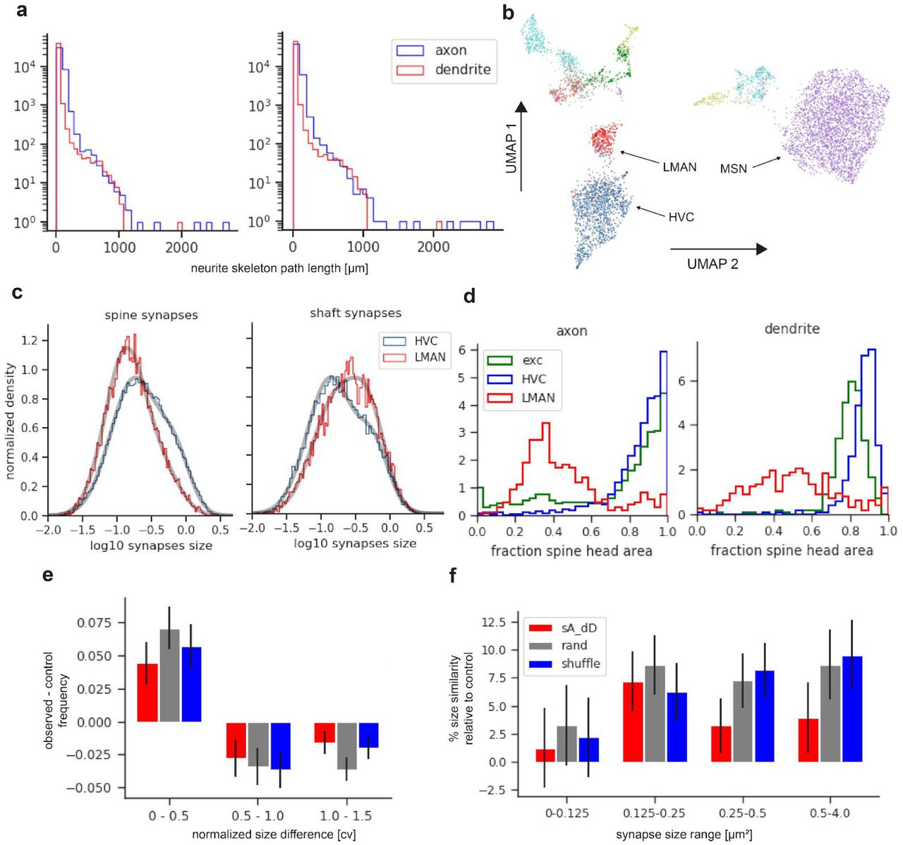
a, MSN dendrite (purple), spine head synapse from an HVC axon (blue arrow), and a shaft synapse from a LMAN axon (red arrow). Same region in cross section (right). Scale bars 1 µm. b, Conceptual sketch of the ratio between spine- and shaft bound-fractions for HVC (top) and LMAN (bottom) inputs and the contribution of each of the four cases to the total excitatory synaptic area on MSN dendrites. c, Normalized histogram of fraction of spine head area per neurite for different axon types with MSN dendrites. d, Same plot from the perspective of MSN dendrites. e, Distribution of log10-transformed synapse size for spine and shaft synapses of HVC and LMAN synapses. Also shown are fits (grey curves) to a model with two log-normal distributions38 (Methods, Extended Data Fig 5).

a, MSN dendrite (purple) that receives two spine-head synapses from the same HVC axon (blue). Also shown in cross sections (right). Scale bars: 1 µm. b, CDF showing the fraction of multi-synaptic area for HVC (blue) and LMAN (red) axons. c, area of the first vs. area of the 2nd synapse (and vice versa, i.e. symmetrized across the diagonal) for all HVC-on-MSN-spine dual pairs. d, Histogram of observed normalized size difference values (cv) for dually connected HVC-MSN spine synapse pairs relative to values for different sets of control synapse pairs. Three different control sets are used: sA_dD, both synapses sampled from the same axon but connecting to different dendrites; rand, control pairs drawn randomly from all HVC-MSN spine synapses; shuffle, control pairs drawn randomly from all dually connected pairs of HVC-MSN synapses, without replacement. Note the excess of pairs with small differences and suppression of pairs with large differences compared to controls. Error bars are  of histogram counts. e, Excess size similarity of HVC-MSN spine synapse relative to controls (percentage mean cv change) for synapse pairs of different mean size ranges. Error bars are s.e.m. (Methods).
We start by analysing the nature of HVC and LMAN synaptic contacts on MSN dendrites (Fig. 2a). Together these inputs contribute 94% of all excitatory synapses onto MSNs. HVC synapses dominate those from LMAN about sixfold by number, and sevenfold by area, a ratio much larger than the 1-to-1 ratio between the numbers of axons (about 10,000) entering from each region36, 37, but smaller than the 12-to-1 ratio between the total axon path lengths (∼90 cm vs. ∼7.7 cm, in the data set; Fig. 2b). Consistent with the model’s prediction, most (86.7%) of the synaptic area of HVC axons onto MSNs was found on spines, while the corresponding fraction was less than half (44.7%) for LMAN axons. Similar results were obtained for sets of manually classified HVC and LMAN axons (87.6% and 38%; 30 neurite fragments each). In contrast, the synaptic areas of HVC and LMAN axons terminating on MSN dendritic shafts were 11.6% and 52.3%, respectively. The fractions of synaptic contact area going to an MSN postsynaptic compartment other than a spine or shaft were negligible (1.4% and 2.5% on somata, and 0.3% and 0.5% on spine necks, for HVC and LMAN, respectively). We found no evidence for distinct subpopulations of HVC or LMAN axons with different spines/shaft ratios; a similar analysis also revealed no distinct subpopulations of MSN dendrites on this basis (Fig. 2c,d).
Given the very different roles for HVC and LMAN synapses postulated in the model, we wondered if these synapses also differ in their distribution of synaptic areas. HVC synapses onto spines were larger than those from LMAN (mean=0.35 µm2 vs 0.22 µm2, median=0.23 µm2 vs 0.15 µm2, n=81,684 and n=8,946, for HVC and LMAN, respectively), while the reverse was true for synapses onto MSN shafts (mean=0.30 µm2 vs 0.35 µm2, median=0.18 µm2 vs 0.25 µm2, n=13,018 and n=6,668, for HVC and LMAN, respectively). These differences were highly significant (two-sided Mann Whitney U tests; all p-values < 10-50). The size distribution of each of the four synapse classes (HVC-spine, HVC-shaft, LMAN-spine, LMAN-shaft) was much better fit by a mixture of two log-normal components than by a single log-normal distribution (Fig. 2e, Extended Data Fig. 5), reminiscent of a similar finding of bimodal synapse sizes in the mammalian cortex38. In fact, the larger size of HVC spine synapses, compared to those from LMAN, is consistent with their hypothesized role in driving temporally specific MSN activity39 and appears to be largely explained by a more robust tendency of HVC synapses to occupy the larger synapse state (HVC-spine: 81% µS = 0.18 µm2; 19% µL=0.71 µm2; LMAN-spine: 89% µS = 0.14 µm2; 11% µL = 0.54 µm2). The converse was true for shaft synapses where it was the LMAN inputs that were more likely to occupy the larger of the two states (HVC: 77% µS = 0.14 µm2 and 23% µL = 0.59 µm2; LMAN: 67% µS = 0.17 µm2 and 33% µL= 0.5 µm2).
In the proposed learning model, LMAN inputs generate a dendrite-wide depolarization to enable detection of HVC and LMAN coincidence. Such broad depolarization might require multiple LMAN contacts spread across the target compartment. We examined the incidence of multi-synaptic connections from HVC and LMAN axons (only fragments > 50 µm long) onto MSN dendrites (Fig. 3a). On average, LMAN axons dedicated 13% of their synaptic area to multi-synaptic connections, while for HVC axons this was only 5%. In both cases, this number is likely to be an underestimate due to a substantial number of reentering axons that result from the limited extent of the data set. About 65% of all LMAN axon fragments, but only 26% of HVC fragments made more than one synapse on the same MSN (Fig. 3b), which is consistent with the more focal distributions of LMAN arbors34. For both HVC and LMAN axons, multiple synaptic contacts had an average pairwise distance of about 10 µm, which is small compared to expected electrotonic lengths.
It has been argued that Hebbian learning should lead to a correlation in the size of synapses that share both pre- and post-synaptic neurons (dual-connection pairs), and that when such correlations are found they constitute evidence for Hebbian learning8, 40, 41. In our data set, the dual-connection pairs (n=1950) between HVC axons and MSN spines showed a significant degree of such size correlations. In particular, the distribution of normalized intra-pair synaptic-area differences was significantly shifted toward smaller values compared to randomized controls (Fig. 3c-e; one-sided Mann Whitney U tests; for all controls p-values < 10-5; see Methods, Extended Data Table 3 and Extended Data Fig. 4). This suggests that HVC-to-MSN-spine synapses, which comprise the vast majority of spinous inputs to MSNs, are capable of Hebbian-type plasticity, consistent with the proposed learning model. For LMAN-to-MSN-spine synapses (n = 443 pairs) a marginally significant effect was observed (shuffle control p-value = 0.045; rand control: p = 0.025; sA_dD control: p = 0.098), while no significant differences from randomized control pairs was seen for shaft synapses of both axon types (all p-values > 0.05; HVC n = 128; LMAN n = 215). Notably, while the enrichment of similarly sized pairs observed in Area X spine synapses is smaller than that observed in hippocampus8, 41, it is comparable to the enrichment reported for neocortex9, 38, 40.

a, Sequence of events (left to right) underlying plasticity at HVC-MSN synapses during vocal learning implemented by a three-factor learning rule. Two HVC axons (left), and multiple synapses from one LMAN axon (right) impinge on an MSN dendrite. Colors indicate: spike activity (yellow), calcium influx (green), eligibility trace (red), and DA release (pink dots). LMAN spiking activity leads to MSN dendritic depolarization; coincident activation of HVC input 1 leads to an eligibility trace in HVC synapse 1. Subsequent arrival of a reward leads to LTP at this synapse (indicated by size increase). After learning, spiking activity in HVC axon 1 leads to MSN activation and improved behavioral output. b, Reinforcement learning of a 1-d vocal output (template, red; learned output, black) over 20,000 iterations, using the proposed learning rule (Methods). c, Left: Comparison of reward signal (DA) in model vs. time course of VTAX neuron responses measured in vivo, with permission, see Gadagkar et al.21. Right: Learning of a single peak, full-width-at-half-maximum: 8.4 ms. d, Average magnitude-squared coherence between template and model output, gray band is s.d.. e, Interpretation of the proposed basal ganglia model for learning in a feedforward network. The fluctuating LMAN output activity is projected back onto the HVC-MSN synapse layer, where the non-plastic feedback signals guide learning at plastic input layer synapses.
To quantitatively assess the ability of the observed neural architecture to correctly implement credit assignment in the context of vocal learning, we constructed a numerical simulation of the model consistent with our anatomical findings. Closely related to the concept of parallel node perturbation7, 15, the local learning rule incorporates non-plastic LMAN shaft synapses, and plastic HVC spine synapses. The latter are strengthened by coincident activation of HVC (state) and LMAN (action) inputs, followed by a delayed reward (Fig. 4a). Numerical simulations show that the model learns to imitate a simple song template after a few thousand iterations (Fig. 4b), consistent with typical learning rates in juvenile zebra finches42. Furthermore, our simulations revealed that the network exhibits a high temporal precision of learning that exceeds that of the reward signal (∼100ms)21 (Fig. 4c), consistent with the reported ∼10 ms resolution of vocal learning in the songbird43 (Fig. 4d).
Connectomic analysis of brain circuitry has shown promise as a method to investigate synaptic plasticity8, 40. Using highly automated dense reconstruction, we have extended this approach to analyze the ultrastructure of synaptic interactions of inputs that carry computationally distinct and learning-relevant signals. In the context of a detailed model of a cortical-basal ganglia circuit that implements reinforcement learning, our data reveal the existence of a significant asymmetry between two types of cortico-striatal (CS) connections. The LMAN input resembles mammalian pyramidal-tract CS projections and carries an efference copy of a motor command signal, while the HVC input resembles mammalian intratelencephalic CS projections and carries a state (timing) signal44, 45. The predominance of HVC inputs onto dendritic spines and LMAN inputs onto shafts supports a model of basal ganglia learning in which action efference copy inputs modulate or gate plasticity of state inputs to MSNs. In this view, MSN spines detect and transiently maintain a memory of recently active action-state pairings.
Our data provide insight into a plausible biological implementation of node perturbation15, a form of stochastic gradient descent learning that performs synaptic credit assignment without backpropagation. Conceptually, our model is a variant that could be called “remote node-perturbation”, since action feedback connections transmit network output variations back to the relevant synapses for credit assignment (Fig. 4e). We have identified a candidate ultrastructural motif for this mechanism: distinct excitatory synapse types interacting on a dendrite to inject variability, to correlate variability with reward signals, and to correctly assign credit to relevant synapses that potentiate improved performance. The generality of such a credit assignment strategy and whether it is anatomically manifested similarly in other brain areas, namely the cortex or the cerebellum, remains an interesting topic for future theoretical and empirical work.
Methods
Code availability
All analysis code will be made available upon publication on GitHub.
Sample preparation
An adult male zebra finch (> 120 days post hatching, obtained from the MPI of Ornithology, Seewiesen, Germany) was transcardially perfused with cacodylate buffer (CB) at room temperature (RT) that contained 0.07 M sodium cacodylate (Serva, Germany), 0.14 M sucrose (Sigma-Aldrich), 2 mM CaCl2 (Sigma-Aldrich), 2% PFA (Serva) and 2% GA (Serva) to retain the extracellular space46. We cut the brain sagittally into 200 µm thick slices on a vibratome (Leica VT1000S), found the slice with the largest cross section of Area X (identified by its round shape and location in the section) and excised a piece of about 300 x 300 µm centered in Area X. We next immersed the sample in a sequence of aqueous solutions in 2 ml Eppendorf tubes. First 2% OsO4 (Serva) reduced with 2.5 % potassium hexacyanoferrate(II) (Sigma-Aldrich) for 2 h at RT, followed by 1% thiocarbohydrazide (Sigma-Aldrich) at 58°C for 1h, then 2% OsO4 at RT for 2h, 1.5% uranyl acetate (Serva) in H2O at 53°C for 2h and 0.02M lead-aspartate (Sigma-Aldrich) at 53°C for 2h. The sample was rinsed three times with CB after the first OsO4 step and once with double-distilled water after each of the other staining steps. We next dehydrated the samples using chilled ethanol-water mixtures (70 %, 100 %, 100 %, 100 %, ethanol (Electron Microscopy Sciences), 10, 15, 10, 10 min) followed by propylene oxide (100%, 100%) (Sigma-Aldrich), infiltrated first with a 50/50 propylene oxide/epoxy mixture, then with 100% epoxy. The epoxy was 812-replacement (hard mixture, Serva). After infiltration, samples were cured (60°C for 48h), trimmed, and smoothed (Leica Ultracut microtome). All animal experiments were approved by the Regierungspräsidium Karlsruhe and were carried out in accordance with the laws of the German federal government.
SBEM data-set generation
The sample was imaged and sectioned in a field-emission scanning electron microscope (SEM, Zeiss UltraPlus) equipped with a custom diamond knife-based serial-blockface ultramicrotome2. We used a landing energy of 1.6 kV, a beam current of 1 nA, a scan rate of 3.3 MHz, a lateral pixel size of 9 x 9 nm and a cutting thickness of 20 nm. The acquired data set (single image tile 10,240 x 10,240 pixels) was initially aligned by translation only, followed by elastic alignment (A. Pope, Google Research. The aligned stack contained 10,664 × 10,914 × 5701 voxels with 8 bit intensity values (∼664 GB). No contrast normalization was performed.
Neuron reconstruction and proofreading
Neurite reconstruction was carried out by Flood Filling Network (FFN) segmentation of the entire (114 µm x 98 µm x 96 µm) data set. Broadly, this was done in two stages: an initial over-segmentation (base segmentation) was created to ensure the near-absence of false mergers; next, segments in the base segmentation were then agglomerated into more complete units. Several steps were taken to improve oversegmentation in the initial stage (i.e. to further reduce the occurrence of false mergers), and to improve object continuity in the second stage (i.e. to reduce the occurence of false splits). In addition to the base segmentation described in Januszewski et al.3, we created an independent new oversegmentation that was then combined with the original base segmentation using oversegmentation consensus3. The new oversegmentation started with the preexisting base segmentation as its initial state. We then used FFN inference with the following adjustments to create new neurite fragments:(a) we increased the “disconnected seed threshold” parameter from 0 to 0.15, which resulted in the assignment of previously unclaimed voxels in the interior of small-diameter axons (36.4B voxels filled); (b) we used a different snapshot of FFN weights (“checkpoint”) in areas with lower data quality (19.8B voxels filled); (c) we recreated objects adjacent to voxels classified as myelin by the tissue type classifier in an FFN inference run without the myelin mask (6.9B voxels filled); and (d) in areas adjacent to detected irregularities we recreated objects in an FFN inference run with FOV movement restriction with the section-to-section shift threshold relaxed from 4 to 6 voxels (1.8B voxels filled). The steps a)-d) were carried out sequentially, and the result of every step was combined with that of the previous step with oversegmentation consensus. To even further reduce the number of false mergers, we took the seed point for every segment in the original base segmentation, and used FFN inference at 2x reduced in-plane resolution to create a segmentation with no encumbrance by any other object (note that in this process the base-set objects can shrink as well as grow). The results were upsampled and combined with the base segmentation, again through oversegmentation consensus.
We then ran FFN agglomeration as described previously3. For every decision point involving at least one segment added in (a)-(d) (see paragraph above), we ran FFN agglomeration a second time, this time with inference settings matching the conditions (a)-(d) under which the segment was created. To detect remaining splits we skeletonized the agglomerated objects using TEASAR47. For each skeleton node with only one adjacent edge we determined whether it was a true neurite endpoint by running FFN segmentation within an empty (no pre-existing segments) (201,201,101)-voxel subvolume centered on the seed placed at the skeleton node. This was done with both the main FFN checkpoint and the one used in condition (b) above. We considered any base segments to be “recovered” if at least 60% of their voxels were overlapped by the predicted object map (POM) generated by the FFN in this procedure, and thresholded at 0.5. We then merged segments (A, B) in case of symmetric recovery, i.e. when the subvolume segmentation described above, seeded from a node located in A recovered B, and vice versa. Finally, we identified orphan fragments (defined as not reaching the surface of the data set) and iteratively (6 times) connected them to the partner fragment with the highest Jaccard score as computed in FFN agglomeration for the fragment pair3. Only pairs for which at most 15% of the voxels of one of the objects changed POM values from >0.8 to <0.5 during FFN agglomeration inference were considered in this step.
The number of orphaned neurite fragments was further reduced by manually inspecting their ends. If a split error was detected, a skeleton tracing was initiated. The annotator was provided with a seed location and an initial tracing direction but not the actual segmentation. Tracing was terminated when the annotator decided that a true neurite ending had been reached or when the newly traced skeleton reached another fragment with > 10 µm skeleton length. The thus created connectors (n=36,154 in 911 hours of tracing) were then used to combine the appropriate fragments. This reduced the number of fragments from 231,207 to 212,656. 13 of those contained at least one erroneous merger, identified by the presence of at least two somata. All connectors contained in those (n=434) were then removed, resulting in 213,076 fragments. This proofreading step was performed using a Python plugin for KNOSSOS (www.knossostool.org).
To further reduce the number of false mergers, one of us (MJ) inspected 36,653 classified neurites using Neuroglancer, identified merge errors by visual evaluation of object shape plausibility, and manually removed agglomeration graph edges causing those mergers. In total, less than 10 hours were spent for this additional proofreading step, which resulted in the removal of 846 edges and the elimination of 840 merge errors.
Unless otherwise mentioned, manual proofreading was performed by student assistants or outsourced (ariadne-service gmbh).
Synapse detection
In a first step, mitochondria, vesicle clouds, synaptic junctions and synapse type were predicted in the data set using two convolutional neural networks4. For each boundary voxel of the FFN segmentation, all other neurite IDs were collected in a 6 x 6 x 3 subvolume and the most frequent ID was denoted the partner neurite ID for this boundary voxel. All voxels that were both part of such a neurite-neurite contact and classified as a synaptic junction were clustered (connected components with a maximum distance of 250 nm) and each cluster considered as a putative synapse object. Mitochondria and vesicle clouds were assigned to the cells with which they shared the highest voxel overlap.
In a second step, every candidate synapse object was assigned a probability by a random forest (RF) classifier trained on manually labeled candidate synapse objects (n=436; non-synaptic: 238, synaptic: 198). Candidate synapses below probability 0.5 were eliminated. This classifier used 11 hand-designed features extracted from the pre- and postsynaptic neuron (collected within a sphere of 4 µm) and from the candidate synapse itself, in particular, the synapse size (in voxels), the volume ratios between contact site and synaptic junction bounding box, synaptic junction and contact site, as well as the numbers and voxel counts of pre- and post-synaptic mitochondria and vesicle clouds.
The synaptic area of identified synapses was estimated as its surface mesh area (which includes pre- and post-synaptic areas) divided by two. Meshes were computed using marching cubes applied to the masked synapse voxels after binary closing with seven iterations.
We used cellular morphology neural networks (CMN)5 to recognize and differentiate cellular substructures. The two models, one for spines5 and one for axons (axon, terminal bouton, en-passant bouton, dendrite, soma; trained on 17 reconstructions; window size of 40.96 µm x 20.48 µm x 20.48 µm and 1024 by 512 pixels; 3 projection windows per location; rendering locations were the set of vertices downsampled by a third of the maximum window size), classified the cell surface based on 2D-projections of the neurite and its mapped organelles (mitochondria, vesicle clouds) and synaptic junctions. Surface labels were mapped to the synapse directly by k-nearest-neighbors in case of spines (k=50). In the axon (dendrite, soma and bouton) case the surface labels were first mapped to the skeleton nodes by k-nearest-neighbors (k=50) and then averaged using a sliding window approach, which collected the labels of skeleton nodes within 10 µm traversal length along the skeleton in every direction starting from the source node. The axon (dendrite, soma, bouton) label of each synaptic partner was taken from the respective skeleton node closest to the synapse.
Cell-type classification
Using the CMN pipeline, we also detected astrocyte fragments, and removed these from all subsequent analyses, as described in5.
The cell types of the remaining FFN reconstructions were then identified with the same approach, with a CMN trained on manually labeled neurites (JK), 30 per class, in total n=240 (HVC, LMAN, MSN, pallidal, subthalamic nucleus like, dopaminergic, cholinergic, interneuron; the dopaminergic and cholinergic classes were combined for the classification used in this manuscript). We modified the CMN from5 by extending the latent representation returned by the last convolution layer with the synaptic area ratio between symmetric and all synapses in the neurite before it was passed to the first fully connected layer. The performance was assessed using ten-fold cross-validation48.
To cluster the neurites for an unsupervised cell type identification, independent of the supervised approach based on the CMN-pipeline, we designed three sets of neurite compartment specific features (soma, axon and dendrite). These consisted of 62 neurite-specific morphology features (e.g., caliber variation, synaptic density, mitochondrial density), as well as 15 features that were computed based on its synaptic connectivity: e.g., for axons, we computed for every of its outgoing synapse a feature of the postsynaptic dendrite, and then used the synaptic area to compute a weighted average of those postsynaptic properties. The full set of features is described in Extended Data Table 1. Each neurite corresponds to a point in this 62 dimensional space which was then projected onto a plane using either the Uniform Manifold Approximation and Projection, UMAP49 or the t-distributed stochastic neighbor algorithm (see Supplementary Note 2)50(Python sklearn.manifold.TSNE) with a random seed of 0. The pairwise distance of two neurites A and B, was calculated by averaging the Euclidean distance of the separate feature vectors of the three compartments (axon, dendrite, soma). In case a compartment did not exist in A or B (compartments with less than 15 synapses associated), it did not contribute to the averaging. The embeddings were visually similar over a range of perplexities (tested from 10 to 320, Extended Data Fig. 2a,b), a parameter which controls in t-SNE how many neighbors should be considered for the embedding, and the actual number of neighbors in UMAP, also a controllable parameter (tested from 10 to 320). After visually inspecting neurites from different clusters and confirming that they agree largely with our supervised results (Fig. 1d; UMAP parameters: n_neighbors=15, min_dist=0.25), we applied Hierarchical density based clustering (HDBSCAN)51 to the down-projected feature space (UMAP parameters: n_neighbors=40, min_distance=0.0; HDBSCAN parameters: min_cluster_size=100, min_samples of 5) to assign cluster labels to each neurite (HDBSCAN clustering on the full feature dimensions led to no meaningful results). Agreement with the supervised CMN classifier was calculated by first identifying for each CMN celltype class the unsupervised cluster label with the greatest overlap that was then compared to the supervised CMN cell type of the same neurite and used to calculate per class F1-scores, shown in Supplementary Note 2.
Synapse-size distribution analysis of HVC and LMAN axons
Synaptic size (contact area) was computed as described in the ‘Synapse detection’ section of the methods.
Synapse sizes were log-10 transformed and the distribution was fit to a mixture of two truncated (lower boundary of 0.01 µm2, no upper boundary) normal distributions (Python scipy.stats.truncnorm) by minimizing the negative log-likelihood function using Sequential Least Squares Programming (Python scipy.optimize.fmin_slsqp). Bayesian Information Criterion (BIC) and Akaike Information Criterion (AIC) comparisons were performed by fitting n-component (n ranging from 1 to 10) normal distributions using Python’s sklearn.mixture.GMM to the log-10 transformed synapse sizes.
We computed the fraction of excitatory synaptic area onto different post-synaptic compartments of MSNs. These fractions were computed separately for synapses arising from HVC, LMAN and STN-like axons as follows. We divided the total synaptic area from one axon class formed onto one MSN post-synaptic compartment class (spine head, neck, dendritic shaft or soma; determined by the morphology classifier5) by the sum of the synaptic area from that axon class onto all MSN compartments. For example, the data set-wide spine fraction for HVC onto MSNs was computed as follows:
 In addition to computing these quantities for the entire data set, we also performed the same analysis restricted to individual axons (Fig. 2c) or MSN dendrites (only for neurites with > 50 synapses) (Fig. 2d). This was done to estimate the distribution of targeted MSN postsynaptic compartments over individual neurites.
Synapse pair size correlation analysis of HVC and LMAN synapses
To identify signatures of Hebbian plasticity we computed several measures of size correlation in synapse pairs with the same pre- and postsynaptic neurites (Fig. 3, Extended Data Fig. 4, Extended Data Table 1). Specifically, 1) we analyzed normalized pair synapse size differences (coefficient of variation), 2) calculated the non-parametric Spearman rank correlation, 3) performed an analysis of variance (ANOVA) and 4) performed a comparison of the variances along the first two principal components.
1) We computed the normalized size difference of the two synapse sizes in a pair (minimum Euclidean distance of 1 µm) as
 with s1 being the larger synapse size in µm2,40. As control we sampled 200,000 pairs randomly from different populations of synapses: synapse pairs that shared the same axon (sA_dD), and random synapse pairs (rand), but all restricted pre-synaptically to either HVC or LMAN axons and post-synaptically to MSN dendrites. The shuffle control pair population was established by performing 1000 random pairings (without replacement) of the observed pair synapse sizes (Fig. 3d,e and Extended Data Fig. 4a-c). Mann Whitney U tests were performed on the cv distributions to assess statistical significance (Python’s scipy.stats.mannwhitneyu).
2) Spearman rank correlation was calculated using Python’s scipy.stats.spearmanr on mirrored pair sizes to account for the arbitrary order of synapses in a pair, i.e. for each pair we considered (s1, s2) and (s2, s1).
3) We further tested for correlated synapse pair sizes using a one-way ANOVA of log10-transformed synapse sizes, and a Kruskal-Wallis test of non-transformed synapse sizes. In both cases, the synapse sizes of a pre-post synapse pair were considered a group, which has the advantage that no artificial ordering has to be introduced, as in the case of the Spearman correlation coefficient. If synapse sizes in pre-post pairs were not independently drawn from the same size distribution, due to a size correlation, the ANOVA test would reject the null hypothesis of no difference in mean between the groups. The same argument applies to the rank based Kruskal-Wallis test (Extended Data Table 3).
4) We projected the mirrored pair synapse sizes on the (1,1) diagonal (s.d.1) and the (−1,1) diagonal (s.d.2) and then calculated the ratio of the standard deviations (s.d.1/s.d.2) along these axes in comparison to the shuffle control (Extended Data Fig. 4e).

Computational model of learning in Area X
A numerical simulation of the basal ganglia circuit underlying songbird vocal learning, focusing on HVC, LMAN, and MSN interactions, was implemented as a firing rate model in Python52. The total song duration was 300 ms (corresponding to a short typical zebra finch song), and the simulation was carried out with 1 ms temporal resolution. The model was implemented with 300 sparsely firing MSNs39, each receiving temporally specific input from a single dedicated HVC neuron that is active at a single 7ms interval in the song (delta-function peak smoothed by a Gaussian kernel with σ = 3 ms, corresponding to a full-width-at-half-maximum of ∼7 ms; activity of adjacent HVC neurons staggered by 1 ms). During singing, the HVC neurons form a continuous sequence53, 54. The LMAN-MSN synapse is assumed to be non-plastic (one axon shared across all MSNs. LMAN activity is generated as random fluctuations between 0 and 1 (smoothed by a 3 ms box kernel). LMAN inputs to MSNs do not activate the MSN, but rather serve to gate plasticity at HVC-MSN synapses. Each HVC-MSN synapse has an eligibility trace defined as
 Where f (t) is a delayed Gaussian kernel with the same width and delay as the DA kernel (see below and Fig. 4c). The weight update rule for HVC-MSN synapses is defined as
 with learning rate β = 2 and a DA signal that depends on the song performance on the current trial compared to recent past trial(s), encoded as performance prediction error ppe(t) (positive when performance is better than expected)
 Where
Where
 and
and
 f (t) is a delayed Gaussian kernel with σ = 42 ms (corresponding to ∼100 ms full-width-at-half-maximum), shifted to peak at 125 ms delay, consistent with experimental findings in the zebra finch21. The vocal output for each iteration was
 where
where
 The vocal output in Fig. 4b,d shows the model output after 20,000 iterations, without the contribution from LMAN, corresponding the zebra finch song in the “directed” social context in which LMAN is known to be relatively silent55. The coherence (Fig. 4d) between the template and the vocal output at the end of learning was computed using Python’s scipy.signal.coherence (parameter nperseg = 64) and averaged over 100 simulations. As an additional test of the temporal resolution of the learning model, the simulation was run again (with identical simulation parameters) with a template consisting of a single peak (7 ms width). The full-width-at-half-maximum of the resulting simulation peak (Fig. 4c) was determined using Python’s scipy.signal.find_peaks and peak_widths.
Data and Code Availability
The source code, aligned EM data, neuron reconstructions, synapse annotations and cellular morphology classifications will be made available upon peer-reviewed publication.
Conflict of Interest
JK holds shares of ariadne-service gmbh. MJ and VJ are employees of Google LLC, which sells cloud computing services.
Contributions
The project was planned by JK, WD and MF. JK prepared the samples, acquired the EM data, as well as performed and supervised: the development of data visualization, annotation, and analysis software, the creation of ground truth data, the analysis of data, and the numerical simulation. MF and JK designed the numerical simulation. WD supervised data acquisition and developed instrumentation with contributions by JK. MJ segmented data with FFNs and proofread segmentation results. PS and JK developed, implemented, and applied synapse detection and classification algorithms. JK, VJ, MJ, PS, WD, and MF interpreted the results and wrote the paper.
Supplementary Note 1 - Analysis of automatically reconstructed connectome
To assess the degree to which the proofreading of the automated reconstructions affected our conclusions, we created a fully automated connectome without manual healing of splits (reconnects) or false mergers. The resulting segmentation contained slightly more neurites (n=46,033 vs. 41,324), due to a higher split rate. This was not offset by the additional false mergers, and had a marginal effect on the overall neurite length distributions (Extended Data Fig. 1a). We recreated key analyses regarding the model predictions, and found virtually no differences (Extended Data Fig. 1 b-d). While our results demonstrate the dramatic progress of automated reconstruction methods for EM data sets, we stress that manual proofreading still improved the quality of the data set. Other connectomic studies requiring more complete circuit-level analysis might still benefit from manual neurite proofreading.
For panels b-f, analyses from panels in main figures are re-computed for data set without manual proofreading. a, Left: Distribution of neurite skeleton path lengths for the manually proofread connectome. Right: without manual proofreading. b, UMAP embeddings of data set neurites, as in Fig. 1d. c, Synapse size distribution of as in Fig. 2e, fitted by two slightly truncated log-normal distributions. d, Normalized histograms of the fraction of synaptic area with spine head synapses for different axon classes, corresponding to Fig. 1c,d. e, Observed pair cv values for dually connected HVC-on-MSN spine synapse pairs minus cv values for different sets of control synapse pairs, as in Fig. 3d. Error bars are  of histogram bin. f, Change of HVC-on-MSN spine synapse size similarity relative to controls as in Fig. 3e. Error bars show relative s.e.m..
Supplementary Note 2 - Cell types
For further validation, we quantified the agreement between our supervised cell type classification method and an unsupervised clustering method on the UMAP down-projected space using HDBSCAN to automatically assign cluster labels (Extended Data Fig. 2c). For HVC, LMAN and MSNs neurites. The agreement F1-scores were 0.96, 0.81, 0.98, respectively, consistent with the mostly uniform coloring of the respective clusters in Fig. 1d.
While not further analyzed in this study, we also identified other neuron types in the data set. Some axon fragments (Extended Data Fig. 2d) resembled a recently described glutamatergic neuron of Area X in their innervation pattern1. The axons formed large asymmetric multi-synaptic contacts with pallidal-like neurons (Extended Data Fig. 2e), which would also be consistent with a reported thalamic projection into Area X2. These other classes of glutamatergic axons are easily distinguished from HVC and LMAN axons by the prevalence of these contacts with pallidal neurons. We furthermore found interneurons forming symmetric synapses, primarily with MSNs. We were able to tentatively identify multiple classes of Area X interneurons on the basis of morphological descriptions in the literature (Extended Data Table 1). Putative cholinergic and dopaminergic axons were similarly identified (Extended Data Table 1). The F1-scores for the supervised CMN classification for all classes were: 0.90 (STN, n=30), 0.93 (modulatory, 60), 0.93 (MSN, 30), 0.95 (LMAN, 30), 0.91 (HVC, 30), 0.96 (GP, 30), 0.91 (INT, 30), the overall accuracy: 0.93 (n=240).

a, UMAP embeddings of all data set neurites with at least 15 synapses (n=7120) with increasing values of the n_neighbors parameter (min_distance=0.1, n_epochs=500). Color labels are based on the Cellular Morphology Neural Network (CMN) cell type classifier: HVC (blue), MSN (purple), LMAN (red), modulatory (light red), subthalamic-nucleus like (green), pallidal-like (yellow), inhibitory interneurons (turquoise) b, tSNE embeddings with increasing values of the perplexity parameter, otherwise as in a. Note how larger perplexity values increasingly reveal global structure in the data, i.e. an increasingly large gap between mostly axonic neurites and mostly dendritic neurites. c, Top: Labels (arbitrary colors) determined by clustering (using HDBSCAN algorithm) on 2d UMAP embedding (n_neighbors=40), to calculate the agreement between the supervised CMN cell type classification method and the unsupervised feature-based clustering. Bottom: Labels determined by naive HDSCAN clustering on full feature space, without parameter tuning. Black neurites represent outliers neurites that were not assigned by HDBSCAN. d, rendering of axon fragment of a subthalamic nucleus-like neuron (red), forming an asymmetric synapse (inset) with the pallidal neuron in e that is densely filled with mitochondria. Synaptic clefts in black, vesicle clouds in green and mitochondria in blue.

a) Renderings of 10 randomly selected HVC axons, b) LMAN axons and c) MSN dendrites. Minimum neurite length 50 µm skeleton path length. The zoomed insets show characteristics of the particular cell types, namely regular boutons for HVC axons, a perforated morphology of LMAN axons, and spiny dendrites of MSNs. Excitatory synapses (red), as determined by the synapse type classifier, mitochondria (blue), vesicle clouds (green). Scale bar is 50 µm.
Cell types and characteristics of neurons.
Compartment specific hand-designed neurite features for clustering; trans-synaptic features, i.e. features that require first-order connectivity information for their calculation with yellow background. Latent features were calculated using a triplet-loss cellular morphology network7.
Statistical analysis of joint pre-post pairs of HVC and LMAN synapses onto MSNs. In shuffle controls random pairs were drawn from the same pre-post pair synapse size pool. Green background: p < 0.01.

Left: Observed pair cv values for dually connected synapse pairs minus cv values for different sets of control synapse pairs, with both synapses sampled from the same axon but connecting to different dendrites (sA_dD) from all synapses (rand); from only synapses in dual pairs (shuffle). Error bars are  of histogram bin. Right: Change of HVC-on-MSN spine synapse size similarity relative to controls (percentage mean cv change) for different pair mean synapses size bins. Error bars show relative s.e.m.. a, for LMAN-on-MSN spine synapses, b, for LMAN-on-MSN shaft synapses and c, for HVC-on-MSN shaft synapses. d, Left: Spearman rank correlation coefficient ρ observed (dashed lines) and for n=1000 shuffles of HVC-on-MSN spine (Spearman ρ = 0.13; p < 10-7) and LMAN-on-MSN spine pair synapses (Spearman ρ = 0.10; p = 0.03); Right: For MSN-shaft synapses, otherwise as in the left panel. e, Left: Ratio of s.d.’s (Methods) observed (dashed lines) and for n=1000 shuffles of HVC-on-MSN spine and LMAN-on-MSN spine pair synapses; Right: For MSN-shaft synapses, otherwise as in the left panel.

a, Gaussian mixture models of HVC on MSN spine synapses (left) and HVC on MSN shaft synapses (right), with underlying truncated normal distributions (synapses below 0.01 µm2 not considered). b, as in a, but for LMAN on MSN spine synapses (left) and LMAN on MSN shaft synapses (right). c and d, Bayesian (BIC) and Akaike Information Criterion (AIC) analysis (lowest score indicates “best fitting” model) of Gaussian mixture models ranging from 1 to 10 gaussian components.
Acknowledgements
Sven Dorkenwald for support with SyConn, Manfred Gahr from the MPI of Ornithology for providing the zebra finches and Jesse Goldberg for VTAX recordings. Ila Fiete, Jesse Goldberg and Jon Shlens for helpful comments on the manuscript. We would also like to thank the KNOSSOS team for programming support, Marius Killinger and Martin Drawitsch for help with the ELEKTRONN library and Julian Hendricks for proofreading of reconstructions. We would like to thank the MPCDF facility in Garching (team of Christian Guggenberger) for compute cluster support and Julia Kuhl for illustrations. This work was funded by the Max Planck Society, Google Research and grant NIH RF1 MH117809.


