

Abstract
Network-based module discovery (NBMD) methods have taken a central role in integrative analyses of omics data in modern bioinformatics. NBMD algorithms receive a gene network and nodes’ activity scores as input and report sub-networks (modules) that are putatively biologically meaningful in the context of the activity data. Although NBMD methods exist for almost two decades, only a handful of studies attempted to compare the biological signals captured by different methods. Here, we first set to systematically evaluate six popular NBMD methods on gene expression (GE) data and Gene-Wide-Association Studies (GWAS). Notably, testing Gene Ontology (GO) enrichment of modules obtained by these methods, we observed that GO terms enriched on modules detected on the real data were often also enriched after randomly permuting the input data. To tackle this bias, we designed the EMpirical Pipeline (EMP), a method that infers the empirical significance of GO enrichment scores of an NBMD solution by computing, for each term, a background distribution of scores on permuted data. We used the EMP to fashion five novel performance evaluation criteria for NBMD methods. Last, we developed DOMINO (Discovery of Modules In Networks using Omics) - a novel NBMD algorithm. In extensive testing on gene expression and genome-wide association study data it outperformed the other six algorithms. As it produces solutions with only a few non-specific GO terms, DOMINO can be used without empirical validation. EMP and DOMINO are available at https://github.com/Shamir-Lab/.
Introduction
The maturation of high-throughput technologies has led to an unprecedented abundance of omics studies. With the ever-increasing availability of genomic, transcriptomic and proteomic data (McLendon et al, 2008; VanderSluis et al, 2018; Zhang et al, 2011), a main challenge remains to uncover biological and biomedical insights by examination of these datasets as a whole (Chen et al, 2019). A leading approach to this challenge relies on biological networks(Aittokallio & Schwikowski, 2006), simplified yet solid mathematical abstractions of complex intra-cellular systems. In these networks, each node represents a cellular subunit (e.g. a protein) and each edge represents a relationship between two subunits (Szklarczyk et al, 2017; Wu et al, 2014; Xenarios et al, 2002) (e.g. a physical interaction between two proteins). Among the many bioinformatics tasks that are tackled by network-based methods, including gene function and drug target predictions (Emig et al, 2013; Warde-Farley et al, 2010), one of the most popular is the discovery of “active” modules in data. Given an omics dataset, network-based module discovery (NBMD) aims to detect subnetworks (i.e. modules) that are functionally relevant (“active”) in the probed biological condition. The core of the NBMD task is to pinpoint highly scoring sets of interacting nodes, where the score of each node (i.e. the activity score) is derived from the data (e.g. log2(fold − change of expression)). As this problem has been proven to be NP-hard (Ideker et al, 2002), many heuristics were suggested to detect active modules (Mitra et al, 2013; Creixell et al, 2015).
An NBMD solution is composed of a set of modules that are enriched for the activity signal. Typically, with a solution at hand, each module is subjected to functional analysis (Eden et al, 2009; Subramanian et al, 2005) wherein the GO (The Gene Ontology Consortium, 2019) functions of the modules genes are assessed. The most popular approach for biologically interpreting a gene set is the Hypergeometric (HG) test, where the proportion of genes annotated for a certain property (GO functional category) in the set is compared to a background set of genes. Applying the HG test to the entire set of the responsive genes in a dataset ignores the modular organization of the response and might miss the more elusive biological signals. In constrast, an NBMD solution can provide a finer understanding of the examined biological conditions and cellular responses by delineating subnetworks that carry out distinct biological endpoints (Leiserson et al, 2015; Cerami et al, 2010). For example, biological responses to stress often comprise the concurrent activation and repression of multiple biological processes, each mediated by a single or a few dedicated signaling pathways (Kyriakis & Avruch, 2012; Ashcroft et al, 2000). NBMD would ideally dissect such a complex response into distinct sub-networks, each representing a certain functional module.
Another key utility of NBMD methods is the amplification of weak signals, where an active module comprises multiple nodes that individually have only marginal scores, but collectively score significantly higher. This ability of NBMD methods is especially critical for the functional interpretation of Genome-Wide Association Studies (GWASs) (Visscher et al, 2012). Numerous GWASs conducted over the last decade have demonstrated that the genetic component of complex diseases is highly polygenic (Khera et al, 2018; Musunuru & Kathiresan, 2019; Sullivan & Geschwind, 2019), affected by hundreds or thousands of genetic variants, the vast majority of which have only a very subtle effect. Therefore, most of the “risk SNPs” do not pass statistical significance when tested individually after correcting for multiple testing (Stringer et al, 2011; Boyle et al, 2017). This stresses the need for integrative approaches that consider multiple related nodes together, and NBMD methods are among the most effective for fulfilling this task (Marbach et al, 2016; Barrenas et al, 2009; Cowen et al, 2017).
Evaluation of NBMD solutions based on GO terms enrichment suffers from a substantial drawback: the lack of ground-truth annotations. The manual cherry-picking (Geistlinger et al, 2019) of the right terms out of those identified, is inevitably subject to researcher bias. Moreover, as different NBMD algorithms tend to capture different biological signals, the underlying functional processes cannot conclusively be determined.
In this study, we first aimed to systematically evaluate popular NBMD algorithms across multiple gene expression (GE) and GWAS datasets based on the enrichment of the called modules for functional GO categories. Unexpectedly, our analysis revealed that algorithms often obtained modules enriched for a high number of GO terms even when run on permuted datasets. Moreover, some of the GO terms that were recurrently enriched on permuted datasets, were also enriched on the original dataset, indicating that NBMD solutions commonly suffer from a high rate of false calls. We therefore designed a procedure for validating the functional analysis of an NBMD solution by comparing it to null distributions obtained on permuted datasets. We used the empirically validated set of GO terms to define novel metrics for evaluation of NBMD algorithms. Finally, we developed DOMINO (Discovery of Modules In Networks using Omics) – a novel NBMD method, and demonstrated that its solutions outperform extant methods in terms of the novel metrics and are typically characterized by a high rate of validated GO terms.
Results
NBMD algorithms suffer from a high rate of non-specific GO term enrichments
We set out to evaluate the performance of leading NBMD algorithms. Our analysis included six algorithms – jActiveModules (Ideker et al, 2002) in two strategies: greedy and simulated annealing (abbreviated JAM_greedy and jAM_SA, respectively), BioNet (Beisser et al, 2010), HotNet2 (Leiserson et al, 2015), NetBox (Cerami et al, 2010) and KeyPathwayMiner (Baumbach et al, 2012) (abbreviated KPM). These algorithms were chosen based on their popularity, computational methodology and diversity of original application (e.g., gene expression data, somatic mutations) (Table S1). As we wished to test these algorithms extensively, we focused on those that had a working tool/codebase that can be executed in a stand-alone manner, have reasonable runtime and could be applied to different data types. Details on the execution procedure of each algorithm are available in the Appendix. We applied these algorithms to two types of data: (1) a set of ten gene-expression (GE) datasets of diverse biological physiology (Table S2) where gene activity scores correspond to differential expression between test and control conditions, and (2) a set of ten GWAS datasets of diverse pathological conditions (Table S3) where gene activity scores correspond to association with the trait (Methods). In our analysis, we used the Database of Interacting Proteins (DIP (Xenarios et al, 2002)) as the underlying global network. Although the DIP network is relatively small - comprising about 3000 nodes and 5000 edges, in a recent benchmark analysis (Huang et al, 2018) it got the best normalized score on recovering literature-curated disease gene sets, making it ideal for multiple systematic executions.
NBMD algorithms included in our analysis.
The ten gene expression datasets used in our benchmark analysis.
The ten GWAS datasets used in our benchmark analysis.
First, applying the algorithms to the GE and GWAS datasets we observed that their solutions showed high variability in the number and size of modules they detected (Figure S1 and Figure S2). On the GE datasets, jAM_SA tended to report a small number of very large modules while HotNet2 usually reported a high number of small modules (Figure S1). jAM_SA tended to report large modules also on the GWAS datasets (Figure S2). Next, we used the hypergeometric (HG) GO enrichment test to functionally characterize the solutions obtained by the algorithms. As part of our evaluation analysis, we applied the algorithms also on random datasets that we generated by permuting the original activity scores. Importantly, we observed that modules detected on the permuted datasets were frequently enriched for GO terms (Figure 1A). Moreover, different algorithms showed varying degree of overlap between the enriched terms obtained on real and permuted datasets (Figure 1B). These findings imply that some - or even many of terms reported by NBMD algorithms do not stem from the specific biological condition that was assayed in each dataset, but rather from other non-specific factors that bias the solution, such as the structure of the network, the methodology of the algorithm and the distribution of the activity scores.

Summary statistics of the solutions obtained on the GE datasets. For each dataset, the number of modules detected by each NBMD algorithm and their sizes are indicated. (Error bars represent 1 SD of the number of genes in modules). The numbers in green are the total number of genes in the union of all modules in the solution.

Summary statistics of the solutions obtained on the GWAS datasets. For each dataset, the number of modules detected by each NBMD algorithm and their sizes are indicated. (Error bars represent 1 SD of the number of genes in modules). We excluded empty solutions. Green numbers are the total number of genes of the union of all modules in the solution.

A. Comparison of GO enrichment results obtained on the original CBX GE dataset and on its permuted datasets. The histograms show the distributions of GO enrichment scores obtained for the modules detected on both datasets. The Venn diagrams show the overlap between the GO terms detected in the two solutions. B. Comparison of GO terms reported on the original and permuted GE and GWAS datasets. We used 1 minus the Jaccard score to measure the dissimilarity between the GO terms. Values close to 1 indicate low similarity between the results on the real and permuted data. Each circle shows, per algorithm, this measure (averaged over ten random permutations) over the 10 datasets. For each algorithm, the datasets are ordered such that higher scores are closer to the center. The gray color represents empty solutions. The results are shown separately for the GE and GWAS datasets.
A permutation-based method for filtering false GO terms
The high overlap between sets of enriched GO terms obtained on real and permuted datasets indicates that the results of most NBMD algorithms tested are highly susceptible to false calls that might lead to functional misinterpretation of the data. We looked for a way to filter out such non-specific terms while preserving the ones that are biologically meaningful in the context of the analyzed dataset. For this purpose, we developed a procedure called the EMpirical Pipeline (EMP). It works as follows: Given an NBMD algorithm and a dataset, EMP permutes the genes in the dataset and executes the algorithm. For each module reported by the algorithm, it performs GO enrichment analysis. The overall reported enrichment score for each GO term is its maximal score over all modules (Figure 2A). The process is repeated many times (typically, in our analysis, 5,000 times), generating a background distribution per GO term (Figure 2B). Next, the algorithm and the enrichment analysis are run on the real (i.e. non-permuted) dataset (Figure 2C). Denoting the background CDF obtained for GO term t by Ft, the empirical significance of t with enrichment score s is e(t) = 1 − Ft (s). EMP reports only terms t that passed the HG test (q-value ≤0.05 on the original data) and had empirical significance e(t) ≤ 0.05 (Figure 2D). We call such terms empirically validated GO terms (EV terms). In addition, for each NBMD algorithm solution, we define the Empirical-to-Hypergeometric Ratio (EHR) as the fraction of EV terms out of all GO terms that passed the HG test (Figure 2E,F).

Overview of the EMpirical Pipeline (EMP) procedure. A. The NBMD algorithm and the GO enrichment analysis are applied on many instances (typically, n=5000) with permuted activity scores. B. A null distribution of enrichment scores is produced per GO term. C. The NBMD algorithm is applied to the original (un-permuted) activity scores, to calculate the real enrichment scores. D. For each GO term, the real enrichment scores is corrected according to its corresponding empirical distribution. In this example, GO_3 passed the HG test, but failed the empirical test and thus was filtered out. E, F. Distributions of HG enrichment scores for all the GO terms that passed the HG test and for the subset of the EV terms obtained on the TNFa expression dataset by jActiveModules with greedy strategy (E) and NetBox (F). The EHR measures the ratio between the number of EV terms and the number of GO terms that passed the HG test. The EHR scores summarize the advantage of NetBox in avoiding false reported terms.
The DOMINO algorithm
While the EMP method is a potent way for filtering out false GO term calls from NBMD solutions, this procedure is computationally demanding, as it requires several thousands of permutation runs. In our analyses, using a 44-cores server, EMP runs typically took several days to complete, depending on the algorithm and the dataset. In order to provide a more frugal alternative that can be used on a desktop computer, we developed a novel NBMD algorithm called DOMINO (Discovery of Modules In Networks using Omics), with the goal of producing confident modules that also lead to high EHR values.
DOMINO receives as input a set of genes flagged as the active genes in a dataset (e.g., the set of genes that passed a differential expression test) and a network of gene interactions, aiming to find disjoint connected subnetworks in which the active genes are enriched. It has four main steps:
0. Dissect the network into disjoint, highly connected subnetworks (slices).
1. Detect relevant slices where active genes are enriched
2. For each relevant slice S
Refine S to a sub-slice S’
Repartition S’ into putative modules
3. Report as final modules those that are enriched for active genes.
Step 0 - Dissecting the network into slices
This pre-processing step is done once per network (and reused for any analyzed datasets). In this step, the network is split into disjoint subnetworks called slices. Splitting is done using a variant of the Newman-Girvan modularity detection algorithm (Girvan & Newman, 2002) (Methods). Each connected component in the final network that has more than three nodes is defined as a slice (Figure 3A).

Schematic illustration of DOMINO. A. The global network is dissected by the Newman-Girvan (NG) modularity algorithm into slices (encompassed in purple line). B. A slice is considered relevant if it passes a moderate HG test for enrichment for active nodes (FDR q ≤ 0.3). C. For each relevant slice the most active sub-slice is identified using PCST (red areas). D. Sub-slices are dissected further into putative modules using the NG algorithm. E. Each putative module that passes a strict enrichment test for active nodes (Bonferroni qval ≤ 0.05) is reported.
Step 1 - Detecting relevant slices
each slice that contains more active nodes than a certain threshold (see Methods) is tested for enrichment for active nodes using the Hypergeometric (HG) test, correcting the p-values for multiple testing using FDR(Benjamini & Hochberg, 1995). Slices with q-values < 0.3 are accepted as relevant slices (Figure 3B).
Step 2a - Refining the relevant slices into sub-slices
From each slice, the algorithm extracts a single connected component that captures most of the activity signal. The single component is obtained by solving the Prize Collecting Steiner Tree (PCST) problem(Johnson et al, 2000) (Methods). The resulting subgraph is called a sub-slice (Figure 3C).
Step 2b - Partitioning sub-slices into putative modules
Each sub-slice that is not enriched for active nodes and has more than 10 nodes is partitioned using the Newman-Girvan algorithm (Methods). The resulting parts, and the sub-slices of ≤ 10 nodes, are called putative modules (Figure 3D).
Step 3 - Identifying the final modules
Each putative module is tested for enrichment for active nodes using the HG test. In this step, we correct for multiple testing using the more stringent Bonferroni correction. Those with q-value < 0.05 are reported as the final modules (Figure 3E).
Systematic evaluation of NBMD algorithms on gene-expression and GWAS datasets
We next carried out a comparative evaluation of DOMINO and the six NBMD algorithms described above (Table S1) over the same ten GE and ten GWAS datasets (Tables S2,S3). This evaluation task is challenging as there are no “gold-standard” solutions to benchmark against. To address this difficulty, we introduce five novel scores for the systematic evaluation of NBMD algorithms. These scores are based on our EMP method and the GO terms that pass this empirical validation procedure. The scores are described in Methods and the results on all algorithms are summarized in Figures 4-6.

EHR and number of reported terms. A. EHR for the GE datasets. B. EHR for the GWAS datasets. C. The number of EV terms reported for the GE datasets. D. The number of EV terms reported for the GWAS datasets. The dots indicate results for each dataset. Error bars indicate the SD across datasets.

Performance measured using the module-level EHR (mEHR) criterion on GE datasets. A. mEHR scores for each algorithm and dataset. Up to ten top k modules are shown per datasets, ranked by their mEHR. B. An example of a module from the solution reported by jAM_greedy on the TNFa dataset (mEHR=0.35). The nodes’ color indicates the logarithm of their fold change in the dataset. The black nodes are the neighbors of the module’s nodes in the network. Right: The EV terms for this module are shown in red and those that did not pass the empirical validation in blue. GO terms with borderline EV score (0.05 < q-val < 0.1) are colored in purple).
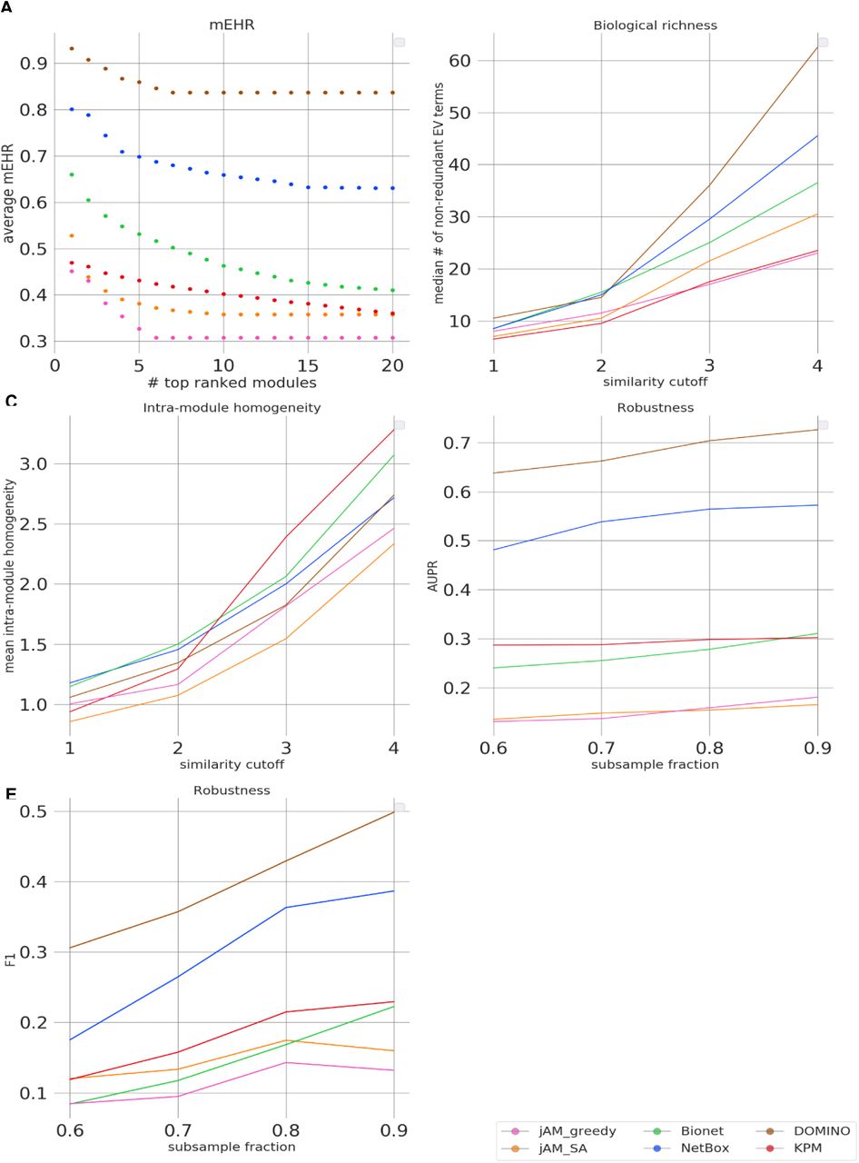
Evaluation results for the GE datasets. A. Module-level EHR scores. The plots show the average mEHR score in the k top modules, as a function of k in each dataset. Modules were ranked by their mEHR scores. B. Biological richness. The plots show the median number of non-redundant terms (richness score) as a function of the Resnik similarity cutoff. C. Intra-module homogeneity scores as a function of the similarity cutoff. D. Robustness measured by the average AUPR over the datasets, shown as a function of the subsampling fraction. E. Robustness measured by the average F1 over the datasets shown as a function of the subsample fraction. For each dataset and subsampling fraction 100 samples were drawn and averaged.
(a) EHR (Empirical-to-Hypergeometric Ratio)
EHR summarizes the tendency of an algorithm to capture biological signals that are specific to the analyzed data, i.e. GO terms that are enriched in modules found on the real but not on permuted data. EHR has values between 0 to 1, with higher values indicating better performance. In our evaluation, DOMINO and NetBox scored highest on EHR. In both GE and GWAS datasets, DOMINO performed best with an average above 0.8. (Figure 4A,B). Importantly, these high EHR levels were not a result of reporting few terms: DOMINO reported a high number of enriched GO terms with only NetBox and jAM_greedy on GWAS reporting more (Figure 4C,D). Since HotNet2, originally developed for analysis of somatic mutation data, yielded poor results on both GE and GWAS datasets we excluded it from subsequent evaluations. For the same reason we included KPM only in the subsequent evaluations of GE datasets.
(b) Module-level EHR (mEHR)
While the EHR characterizes a solution as a whole by considering the union of GO terms enriched on any module, biological insights are often obtained by functionally characterizing each module individually. We therefore next evaluated the EHR of each module separately. Specifically, for each module, we calculated the fraction of its EV terms out of the HG terms detected on it (Methods). The results are summarized in Figure 5A. Notably, solutions can have a broad range of mEHR scores (see, for example, NetBox solution on the IEM dataset, where the best module has an mEHR above 0.9 while the poorest has an mEHR below 0.2). To summarize the results over multiple modules, we averaged the k top scoring modules (using k=1 to 20; Figure 6A). In this criterion, DOMINO got highest mEHR scores for most values of k, followed by NetBox. The results for GWAS datasets are shown in Figure S3A and Figure S4A.


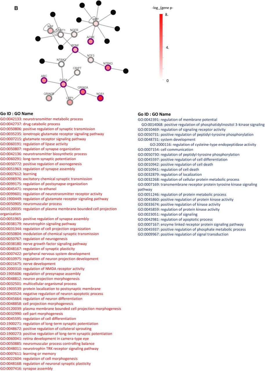
Module-level EHR (mEHR) scores on the GWAS datasets. A. mEHR scores for each algorithm and GWAS dataset. B. An example of a module from the solution reported by DOMINO on the Schizophrenia dataset (mEHR=0.8), and its enriched GO terms. The nodes are color coded by their gene scores as calculated by PASCAL (Lamparter et al, 2016) and -log10 transformed. Black nodes are the neighbors of the module’s nodes in the network. Nodes with purple border are active nodes (qval < 0.05). Red: top 50 EV terms. Blue: enriched HG terms that failed the empirical test.

Evaluation results for the GWAS datasets. A. Module-level EHR scores. The plots show average mEHR score in the k top modules, as a function of k. Modules are ranked by their mEHR scores. B. Biological richness. The plots show the median number of non-redundant terms (richness score) as a function of the Resnik similarity cutoff. C. Intra-module homogeneity scores as a function of Resnik similarity cutoff. D. Robustness measured by the average AUPR over the datasets, shown as a function of the subsampling fraction. E. Robustness measured by the average F1 over the datasets shown as a function of subsample fraction (results for each dataset and fraction were averaged over 100 subsampling).
Furthermore, the EMP procedure enhances the functional interpretation of each module by distinguishing between its enriched GO terms that are specific to the real data (i.e., the EV terms) and those that are recurrently enriched also on the permuted ones.This utility of EMP is demonstrated, as one example, on a module detected by jAM_greedy on the TNFa GE dataset (Figure 5B). TNFa is a potent inducer of immune reponses largely mediated by the NFκB transcription factors. This biological process is well captured by the GO terms that passed EPM validation (e.g., “NIK/NF-kappaB signaling”) (Hayden & Ghosh, 2014). In contrast, GO terms that failed passing this validation procedure represent less specific processes (e.g., “regulation of RNA biosynthetic process”). Similarly, EV terms of a module detected by DOMINO on the schizophrenia GWAS data are highly relevant for this trait (e.g., “neurotransmitter metabolic process”, “regulation of neurogenesis” and “learning”) (Ripke et al, 2014) while GO terms that did not pass validation are either generally less specific (e.g., “system development” and “regulation of localization”) or seem less relevant biologically (e.g., “regulation of apoptosis”) (Figure S3B).
(c) Biological richness
The next criterion aims to measure the diversity of biological processes captured by a solution. Our underlying assumption here is that the biological systems are complex and their responses to triggers involve the concurrent modulation of a diversity of biological processes. For example, genotoxic stress concurrently activates DNA damage repair mechanisms and apoptotic pathways and suppresses cell-cycle progression. However, merely counting the number of EV terms of a solution would not faithfully reflect its biological richness because of the high redundancy between GO terms. This redundancy stems from overlaps between sets of genes assigned to different GO terms, mainly due to the hierarchical structure of the ontology. We therefore used REVIGO(Supek et al, 2011) to derive a non-redundant set of GO terms based on semantic similarity scores(Lord et al, 2003),(Resnik, 1999). We defined the biological richness score of a solution as the number of its non-redundant EV terms (Methods). The results in Figure 6B show that on the GE datasets, DOMINO and NetBox performed best. On the GWAS datasets, jAM_greedy performed best (Figure S4B).
(d) Intra-module homogeneity
While high biological diversity (richness) is desirable at the solution level, a single module should ideally capture only a few related biological processes. Solutions in which the response is dissected into modules where each represents a distinct biological endpoint are easier to interpret biologically and are preferred over solutions with larger modules, where each represents several composite processes. To reflect this preference, we introduced the intra-module homogeneity score, which quantifies how functionally homogeneous the EV terms captured by each module are (Methods). For each solution, we take the average score of its modules. On the GE datasets, BioNet and NetBox performed best in this criterion for the lower similarity cutoffs while KPM scored the highest for the higher cutoffs (Figure 6C). On the GWAS datasets, NetBox, DOMINO, and jAM_greedy scored higher than jAM_SA and BioNet (Figure S4C).
(e) Robustness
This criterion measures how robust an algorithm’s results are to subsampling of the data. It compares the EV-terms obtained on the original dataset with those obtained on randomly subsampled datasets. Running 100 subsampling iterations and using the EV terms found on the original dataset as the gold-standard GO terms, we compute AUPR and average F1 scores for each solution (Methods). DOMINO’s solutions showed the highest robustness on the GE datasets, followed by NetBox (Figure 6D,E). It also performed best on the GWAS datasets, showing markedly higher robustness than all other algorithms (Figure S4D,E).
Table 1 (and Table S4) summarizes the results of the benchmark on GE and GWAS datasets. For the GE datasets, DOMINO performed best in five of the six criteria, while KPM scored highest in intra-module homogeneity. On the GWAS datasets, DOMINO scored best in four criteria, while jAMgreedy had the highest biological richness and NetBox had the highest intra-module homogeneity. Overall, these results demonstrate the high performance of DOMINO in multiple solution facets in both GE and GWAS datasets. NetBox tended to give the second-best results overall.
Summary of the standard deviation of the results in Table 1
Summary of the benchmark results.
Discussion
The fundamental task of network-based module discovery (NBMD) algorithms is to identify active modules in an underlying network based on genes activity profiles. The comparison of such algorithms is challenging due to the complex nature of the solutions produced. Algorithms differ dramatically in the number, size, and properties of the modules they detect. Although NBMD algorithms have been extensively used for some two decades, there is no accepted community benchmark and no consensus evaluation criteria have emerged. Since modules are often used to characterize the biological processes that are activated/repressed in the probed biological conditions, we analyzed the solutions produced by the algorithms from the perspective of functional enrichment. Early on, we observed that many enriched GO terms also appear on permuted datasets, suggesting that such enrichments stem from some proprieties of the algorithms or the data that bias the results. Following this observation, we developed the EMP procedure, which empirically calibrates the enrichment scores and filters out non-specific terms.
Our analysis highlighted the need for improved NBMD algorithms and better benchmark methodology. We developed the DOMINO algorithm and defined five novel evaluation criteria to allow systematic comparison of NBMD algorithms. Each of these criteria emphasizes a different aspect of the solution (Figure 7). We used these criteria to evaluate the performance of six popular NBMD algorithms and our DOMINO algorithm on a set of ten GE and ten GWAS datasets that collectively cover a very wide spectrum of biological conditions. Overall, DOMINO performed best, indicating its ability to produce “clean”, stable and concise modules. NetBox also scored high in our evaluation analysis. Interestingly, both DOMINO and NetBox handle the activity scores as binary ones. Intuitively one may expect that such a step could lead to a loss of important biological signals. However, the high performance of these algorithms suggests that at least on our benchmark binarizing the data helped in reducing noise. Further study of this observation is needed.

A breakdown of the evaluation criteria by their properties. Richness, EHR and robustness score solutions based only on the whole set of the reported GO terms, without taking into account the results for individual modules. In contrast, mEHR and intra-module homogeneity score solutions in a module-aware fashion. From another perspective, biological richness and intra-module homogeneity consider the functional relations among the reported GO terms, while EHR, mEHR, and robustness do not. Colors highlight the different facets considered by each group of scores.
Notably, the algorithms that we tested differ substantially in their empirical validation rates (i.e., EHR). Some algorithms produced solutions with very low EHR (<0.5), and therefore running the EMP on them is critical. While empirical correction is desirable and adds confidence to the reported results, it is computationally highly demanding even with a relatively small network (DIP). Using larger networks, of course, makes this procedure even slower. A notable advantage of DOMINO is the high validation rates it consistently obtained: its average EHR and average mEHR were above 0.8. This indicates that DOMINO can be confidently run without EMP when computational resources are limited. The EMP and DOMINO software and codebases are freely available to the community at https://github.com/Shamir-Lab/.
One shortcoming of EMP is that it does not lend itself to provide module-based correction for enrichment scores, since each randomized run can produce a different number of modules of different sizes. Ideally, one would like to validate the GO terms on the module level. Nevertheless, we do provide means for validation of terms on the module-level by the mEHR index, which calculates the proportion of enriched GO terms that passed the EMP filter in each module. Another limitation is the speed, which also limits the size of networks one can use.
An additional future task is to understand better the sources of the bias that causes over-reporting of enriched GO terms. The sources may be the activity score distribution, network structure, algorithm strategy, etc. Obtaining such understanding could lead to improved module discovery and shorter runtimes of EMP. It could also enable tuning of each algorithms’ hyper-parameters, which is another open issue in our analysis.
In summary, in this study we (1) report on a highly prevalent bias in popular NBMD algorithms that leads to non-specific calls of enriched GO terms, (2) implemented a procedure to allow for the correction of this bias, (3) introduced novel evaluation criteria of solutions and (4) developed DOMINO – a novel NBMD algorithm with low rate of non-specific calls and better performance across most of the criteria.
Methods
1. The Newman-Girvan algorithm in DOMINO
The Newman-Girvan (NG) algorithm is a community detection method(Girvan & Newman, 2002). This method iteratively removes edges using the Betweenness-centrality metric for edges and recomputes the modularity score for each intermediate graph. Let Mi be the modularity score for the graph in iteration i. The process continues until a stopping criterion is met. The stopping criterion we used in DOMINO’s step (1) is that Mi+1 ≤ Mi. For step (2b), the stopping criterion is  . For more details see Appendix.
2. Threshold for testing relevant slices
Slices that contain only a few active nodes are unlikely to be relevant. Testing multiple such slices would diminish the significance of the actual relevant slices. Therefore, we test for relevance only slices that satisfy either
 or
or

3. The PCST application in DOMINO
In PCST (Johnson et al, 2000), nodes have values called prizes, and edges have values called penalties. All values are non-negative. The goal is to find a subtree T that maximizes the sum of the prizes of nodes in T minus the sum penalties of the edges in it, i.e., ∑v∈T p(v) − ∑e∈T c(e) where p(v) is the prize of node v, and c(e) is the cost of edge e.
The node prizes are computed by diffusing the activity of the nodes using influence propagation with the linear threshold model(Kempe et al, 2015). The process is iterative: Initially, the set of active nodes is as defined by the input. In each iteration, an inactive node is activated if the sum of the influence of its active neighbors exceeds θ = 0.5. The influence of a node that has k neighbors on each neighbor is  . Activated nodes remain so in all subsequent iterations. The process ends when no new node is activated. If v became active in iteration l then p(v) = 0.7l. We define the penalty of edge e as c(e) = 0 if it is connected to an active node, and c(e) = 1 − ϵ otherwise (we used ϵ = 10−4).
PCST is NP-hard but good heuristics are available. In DOMINO we used FAST-PCST (Hegde et al, 2014). The resulting subgraph obtained by solving PCST on each slice is called its sub-slice. See Figure 3C.
4. Derivation of p-values and q-values for the GE and GWAS datasets
For the GE datasets, we calculated p-values for differential expression between test and control conditions using edgeR (Robinson et al, 2010) for RNAseq and student t-test for microarray datasets. We computed q-values using Benjamini-Hochberg FDR method (Benjamini & Hochberg, 1995). For GWAS we took the p-values of each SNP for the significance of its association with the analyzed trait and summarized them to gene-level p-values with PASCAL (Lamparter et al, 2016), using the sum chi-square option and flanks of 50k bps around genes. We computed q-values using Benjamini-Hochberg FDR method (Benjamini & Hochberg, 1995).
5. NBMD tools - execution details
See the Appendix for details on the execution of each of the six algorithms benchmarked.
6. Criteria for evaluating NBMD solutions
We defined five novel criteria to allow systematic evaluation of solutions provided by NBMD algorithms. For a specific solution, we considered the list of GO terms that passed the HG enrichment test (HG terms) and the terms that passed the EMP validation procedure (EV terms).
Solution-Level Criteria
(1) Empirical to Hypergeometric Ratio (EHR)
We define the Empirical-to-Hypergeometric Ratio (EHR) as the ratio between the number of reported HG terms and EV-terms. EHR summarizes the tendency of an algorithm to over-report GO terms, with values close to 1.0 indicating good solutions while values close to 0 indicating poor ones. EHR reflects the precision (true positive rate) of a solution.
(2) Biological Richness
This criterion quantifies the biological information collectively captured by the EV-terms. As often there is high redundancy among enriched GO terms - mainly due to the hierarchical structure of the GO ontology - we use the method implemented in REVIGO(Supek et al, 2011) to derive a non-redundant set of EV terms, that is, a measurement of the biological diversity of the solution. This method is based on a similarity matrix of GO terms, which is generated using Resnik similarity score (Resnik, 1999). The biological richness score is defined as the number of non-redundant EV terms in a solution. We calculated this measure using different similarity cutoffs (1.0 to 4.0 in REVIGO).
(3) Solution Robustness
This criterion evaluates the robustness of a solution to incomplete gene activity data. It compares the EV-terms obtained on the original dataset with those obtained on randomly subsampled datasets, where non-sampled gene levels are treated as missing. We repeated this procedure for subsampling fractions 0.6, 0.7, 0.8, and 0.9, iterating each fraction 100 times. Using the EV terms of the full dataset as the truth, we then computed average precision, recall and F1 scores across these iterations. Another perspective is provided by the examination of the frequency by which GO terms are detected in the subsampled datasets: higher frequency for a specific EV-term implies higher robustness. We measured this robustness aspect of a solution using AUPR, in which EV terms are ranked according to their frequency across iterations, and EV terms detected on the full dataset are used as the positive instances). Note that cases in which an algorithm results in many empty solutions (that is, solutions with no enriched GO terms) and a few non-empty ones that are enriched for true EV terms can yield a high but misleading AUPR score. Therefore we validated that the fraction of non-empty solutions obtained by the algorithms on the subsampled runs is high: all the algorithms achieved around 70% or more non-empty solutions on GE data (Figure S6).
Module-Level Criteria
(1) Module-Level EHR (mEHR)
This criterion calculates a single module’s EHR. We define the module-level EHR (mEHR), as the ratio between the number of a module’s EV terms and HG terms (Figure S5A). We score each solution by averaging the mEHR of its k top-ranked modules (k values ranging from 1-20).

Module-level evaluation criteria. A. mEHR. Enriched GO terms in each module are examined by the EMP procedure (EV terms are colored in red) and mEHR is calculated for each module in the solution. B. Intra-module homogeneity. A GO graph is first built for the union of all the EV terms in a solution using Resnik similarity scores. Then, a certain cut-off is applied (here, 4.0) for filtering low scoring edges. Last, the intra-module homogeneity score is calculated as the density ratio between the EV terms that are enriched in the module and the entire GO graph

The fraction of non-empty solutions as a function of the subsampling fraction. For each algorithm and subsampling fraction we report the average over the datasets.
(4) Intra-Module Homogeneity
This index measures the homogeneity of the biological signal that is captured by each module compared to the biological signal in the entire solution. For its calculation, we build a (complete) graph for the solution’s EV terms (GO graph) in which nodes represent the EV-terms and the weights on the edges are the pairwise Resnik similarity score (Figure S5B). Next, edges whose weight is below a cutoff are removed. The intra-module homogeneity is defined as the module’s relative edge-density:

We calculate the intra-module homogeneity score for a solution by averaging its modules’ scores (Figure S5B). We repeat this test for a range of similarity cutoffs – from 1.0 to 4.0. This criterion provides a complementary view on top of the one captured by the biological richness criterion, by characterizing its the biological coherence of the reported modules.
Funding
Study supported in part by German-Israeli Project DFG RE 4193/1-1 (to RS and RE), by the Israel Science Foundation grants No. 1339/18 (to RS) and 2118/19 (to RE), by Len Blavatnik and the Blavatnik Family foundation (to RS) and the Koret-UC Berkeley-Tel Aviv University Initiative in Computational Biology and Bioinformatics (to R.E.). HL was supported in part by a fellowship from the Edmond J. Safra Center for Bioinformatics at Tel-Aviv University. R.E. is a Faculty Fellow of the Edmond J. Safra Center for Bioinformatics at Tel Aviv University.
Appendix 1: NBMD tools - execution details
The NBDM algorithms that we tested differ in preprocessing, input and output. We describe below the specific execution details for each algorithm.
jActiveModules
(Ideker et al, 2002). jActiveModules was written as a plugin for Cytoscape (Shannon et al, 2003), a powerful platfrom for network analysis of biological data. We modified the codebase of jActiveModules so we could run it independently of Cytoscape. jActiveModules expects a list of genes and their p-values as the gene activity scores. We increased the default number of requested modules (from n=5 to n=50) to retrieve more modules and required that reported modules would be mutually exclusive. The algorithm typically producing no more than 10 modules with more than 3 genes.
NetBox
(Cerami et al, 2010). We modified NetBox codebase so we can choose the networks it uses. NetBox gets as an input a list of mutated genes, that is, binary gene activity scores. We used the genes’ q-values and set the gene score to 1 if its q-value was < 0.05, and 0 otherwise.
BioNet
(Beisser et al, 2010). BioNet is designed to retrieve only one module. To retrieve multiple mutually exclusive modules we executed BioNet iteratively, removing the genes in the identified module in each iteration. We stopped these iterations after retrieving modules smaller than four genes in five consequtive runs.
HotNet2
(Leiserson et al, 2015). HotNet2 expects gene activity scores that are calculated by mutation rate p-values (e.g., using MutSig). We transformed the q-values calculated from our datasets into – log10(q_value) scale and used them as the input activity scores. We considered all the reported modules, ignoring their scores reported by HotNet2.
KeyPathwayMiner
(Baumbach et al, 2012). We used the version of KPM with the greedy strategy. It expects binary gene activity scores: 1 marks a gene as active and 0 otherwise. We used the genes’ q-values and scored a gene with 1 if its q-value was < 0.05, and 0 otherwise. As the reported modules considerably overlap each other, we executed the algorithm iteratively, removing in each iteration the genes in the identified module.
DOMINO
DOMINO gets as an input a set of active genes, that is, binary gene activity scores. We used the genes’ q-values and set the gene score to 1 if its q-value was < 0.05, and 0 otherwise.
The Newman-Girvan (NG) algorithm
The Newman-Girvan method (Girvan & Newman, 2002) iteratively removes edges using the Betweenness-centrality metric for edges. This method iteratively removes edges using the Betweenness-centrality metric for edges. Betweenness-centrality scores each edge according to its frequency in shortest paths between all node pairs. For each node pair, a shortest path is calculated and a score of 1 is added to each edge that appears in the path. For node pairs with multiple shortest paths the score is split evenly among the different paths (e.g. a node pair with two shortest paths will add 0.5 to the score of an edge for of each appearance of the edge in any of the paths). The highest scoring edge is thereafter removed from the graph and the process repeats. In some iterations, the process breaks connected components into smaller ones. The overall solution at iteration i is given a “modularity score”, which measures how well-connected are the nodes inside each CC, while being disconnected from nodes in other CCs. Mi is calculated as follows:

Where NM is the number of modules (connected components in the current graph), ls is the number of edges within modules, L is the total number of edges in the network, and ds is the sum of the degrees of all nodes within modules. Originally, the algorithm reports the partition that is associated with the highest modularity score. In DOMINO, the process continues until a stopping criterion is met. The stopping criteria we use in DOMINO are:

References


