

Abstract
Regression analysis is a mature body of knowledge, but there might be room for one more strategy with advantages regarding a class of problems common in modern medical research. Specifically, modern lines of investigation often involve several tens or a few hundred subjects but several hundred assays of cryptically related markers (e.g. blood plasma proteins for ~100 patients vs the same for ~100 unaffected persons). The class arises because research is expensive and sometimes carries a degree of risk to subjects. Also, reliable interpretation of results may employ not just a set of individually distinguished markers, but networks of related markers that are collectively—but not so much individually—informative. This article explores a linear regression strategy that chooses markers parsimoniously but also calculates weights robustly in the sense that both marker choices and weights are generally invariant with respect to small changes in input data. Furthermore, the method allows integration of markers of very different types, thereby improving classification performance and suggesting etiologies and treatments.
Introduction
In real Euclidean n-dimensional space, linear regression finds a classifier for a set of n subjects (e.g. binary case/control status), that is, a sum of marker vectors that approximates by some metric a target vector. For example, the sum might have relatively large values for cases and relatively small values for controls. Converting the values of each marker to z-scores simplifies approximation of a binary target. For a nonbinary targets entries in the target vector itself could be converted to z-scores.
Regression modeling strategies for choosing the weights in a weighted sum already comprise a mature and extensively documented body of statistical knowledge1. The basic idea of ordinary (linear) least-squares optimization is minimization of the sum of the squares of differences of target values and sum values. Finding optimal weights is an application of algebra and calculus dating to the early 1800s and works of Legendre and Gauss. Related strategies include those that optimize some metric other than a sum of squares of errors such as Tikhonov regularization (or ridge regression) and LASSO (least absolute shrinkage and selection operator)1. LASSO has the great advantage of using parsimonious choice of markers, thus avoiding use of many or all markers with inexplicable weight values. And while complicated methods can fit training data very well or even perfectly, the solution often performs poorly on external data—a consequence of overfitting.
Furthermore, as Hand has argued2,3, devising additional methods to solve a specific data classification problem until one finally outperforms another is merely “the illusion of progress”. Therefore, there is a substantial burden of proof of utility attending proposal or use of an exotic regression model.
The popular and powerful LASSO algorithm (with the least angle regression selection (LARS) algorithm) is available as the “alpha = 1” option within the Elastic Net of glmnet4–6; R scripts reside in The Comprehensive R Archive Network at https://cran.r-project.org/. Considering the acknowledged value of LASSO, the emphasis herein will be on comparisons with LASSO as the “gold standard”. Beyond comparisons, some background theory will be provided that explains why our novel method outperforms LASSO.
Weights in linear approximations
Any conventional method (including LASSO) that computes real weights will generally not compute from two experiments exactly the same real weights. This presents the experimenter with the problem of determining exactly how much value a particular marker contributes to the classifier, all compounded by questions about how much effort is justified in obtaining more or less accurate marker measurements, and so on.
Perhaps surprisingly, this note advocates choosing weights that are +1, −1, or (default) 0. This “coarse approximation linear function” (CALF) might seem at first as hopelessly primitive and unlikely to compete with any recognized linear regression method. But CALF can:
equal or surpass LASSO as a classifier of a binary target, that is, select about the same or fewer nonzero markers, using only coarse weights +1, so that for the same problem CALF approximations have superior mean squared error (mse), area under curve (AUC) of receiver operating characteristic (ROC), and Student t-test p-value.
achieve good approximations with coarse weights that are often unchanged by small changes in real-valued marker data.
be applied with analogous advantages to approximation of nonbinary targets where the goal is a parsimonious selection of markers that, when summed, yield a result with high Pearson correlation to (normalized) values of a real-valued target.
offer a significant improvement over LASSO in subsequent permutation tests (described below).
The CALF algorithm
The underlying task includes a target vector of values, one for each subject, represented as a column matrix. The data matrix has a row for each subject and a column for each marker. Thus, a weight vector (row matrix) multiplied by the data matrix should, by some metric, resemble the target. If the target is binary with, say, 0 = control and 1 = case, then the control values in the product should be generally lower than the case values; that would imply low pval.
We call the basic greedy algorithm (a simple version of forward selection linear regression) used herein the “Coarse Approximation Linear Function algorithm” (CALF). CALF selects one by one a limited set of markers and adds them using +1 weights to make a classifier.
We start with binary (dichotomous) CALF in which the target vector has 0, 1 entries, say, 0 for controls and 1 for cases. The raw markers are real-valued vectors which have been initialized into z-scores. CALF finds a sum that for control targets has relatively low values and for case targets relatively high values. The one by one selection is greedy; at each step, it simply tests all the unselected markers, trying +1 weights, to find a marker and weight that improves a metric at least as well as any other selection. Considering each iterative sum as a tentative classifier, the metric can be the Student t-test p-value (pval) or the area under curve (AUC) of the receiver operating characteristic (ROC).
As an algorithm using pval (using AUC is analogous), CALF is therefore the following.
Initialize data = a n-dimensional binary target vector and sorted unselected set = nonempty set of n-dimensional marker vectors
pval = 1
CALF sum of markers = 0 vector as initial target vector output
selected set of markers = empty
one at a time, add to the current CALF sum the vector value of each marker from the unselected markers with weight +1 to update the CALF sum and repeat with weight −1. Note the resulting pval for each of the 2n sums.
if no updated pval is smaller (an improvement) than the stored value, then END
else, choose a marker with maximal improvement and store as a pair it and its weight in the selected set; remove the same marker from the unselected set
store also as a pair the updated CALF sum and the value of the improved pval
if the new number of selected markers = limit, then END
else, if the unselected set empty, then END
else, go to 1.
If instead AUC is a preferred metric, then the initial value is 0.5. The algorithm seeks to increase AUC with each iteration.
Why does CALF work?
Components of the CALF function are suggested by Figure 1
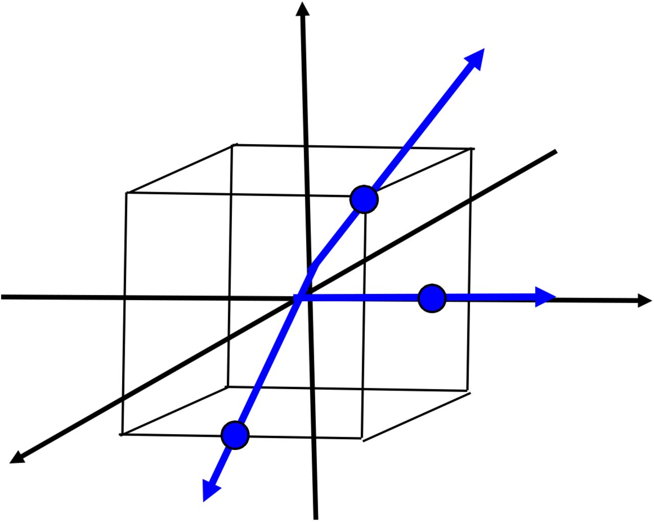
Three rays employed by CALF in 3-dimensional space.
We define in 3-dimensional space a standard cube by its vertices, namely, all points with coordinates that are combinations of +1. In three-dimensional space there are 26 rays from the origin passing through those vertices, the midpoints of edges, or the midpoints of (square) faces of the cube. For clarity, only three representative rays of the 26 are shown in Figure 1. The surface area of the cube is 24, so the ratio of possible CALF rays to area is 26/24.
Generalizing the concepts in Figure 1 to n-dimensional space, there are 3n-1 such rays passing from the origin through all points with coordinates that are combinations +1, −1, or 0. The area of the standard n-cube is n2n. Thus, the ratio of the number of all possibly CALF rays to surface area is (3n-1)/(n2n). It can be shown using calculus that in dimensions ≥ 4, this ratio exceeds 1.05n. Roughly speaking, the rays available to CALF approximations become “exponentially crowded” as dimension increases.
To elaborate on the diversity of directions available to CALF, we note that in any type of regression, specification of weights for w marker vectors, each n-dimensional, corresponds to selection of a w-dimensional weight vector. An approximation of the ith entry in the n-dimensional target vector is the dot product of that weight vector and the vector of ith entries of marker values. If the target vector is represented as a column matrix, then the approximation is the matrix product of an n-by-w matrix of marker data with the weight vector also represented as a column matrix. If components of the weight vector are selected from (+1, −1,0), then in, say, 20-dimensional space, 320-1 = ~3.49E9 selections are possible. Weight vectors can be thought of as providing an approximation of all the possible real-valued “directions” (rays) in 20-dimensional weight space. For the pval (or AUC) metrics, only direction of the weight vector, not magnitude, is significant.
To make the “crowding” argument more quantitative, suppose we generate two real 20-dimensional vectors A and B with uniformly random (real valued) components in [-1, +1]. From A, form a coarse vector Ac such that the ith component Ai, i= 1, 2, ., 20, of Aci is:

Thus, each entry in the coarse vector is just the corresponding entry in A rounded into three bins. Let us divide the n-dimensional vectors A, B, and Ac by their lengths to form vectors of unit length A, B, and Ac. Finally, we form a pair of dot products: A·B and Ac·B.
If we do generate random A and B 1000 times, we get 1000 pairs of such dot products with values in the range [-1, +1]. How do the pairs of dot products differ? In one simulation, the average absolute value in 1000 trials of the pairwise differences of dot products A·B and Ac·B, that is, |A·B − Ac·B|, was 0.054 (SD = 0.041). Upon forming from the 1000 dot products two 1000-dimensional vectors of dot products, the correlation in 1000-dimensional space was 0.94. One could say that overall, the dot products using A or the coarse Ac with B are quite similar. Starting over in either 10-dimensional space or 100-dimensional space (the numbers of subjects back in the regression setting), graphs in Figure 2 compare the first 100 pairs of dot products and provide a visual indication of their similarity. Trials with other, larger dimensions and many more numbers of dot products show the same similarities.

Good approximations of dot products using coarse weights. (1) Shown in random order for 10-dimensional space are representative (first 100) comparisons of 1000 trials. Each trial generated two dot product values as described in the text. (2) The same for 100dimensional space.
Over 10000 iterations of the simulation of 10-dimensional dot product comparisons, the ranges of A·B and Ac·B values were observed to be about [-0.95, 0.93] and [-0.95, 0.94]. The average difference |A·B − Ac·B| was about 0.084 with SD 0.063. For the same experiment in 100dimensional space, ranges were about [-0.37, 0.36] and [-0.35, 0.37], and the average of |A·B − Ac·B| was about 0.027 with SD 0.020.
In summary, outcomes of representative experiments in Figure 2 indicate the dot products of two real, random vectors of unit length are close to the dot products when one has been rounded coarsely into three bins, as above.
Classifier goals
Our three goals are:
Choose automatically a parsimonious set of informative markers from a large set of potential markers.
Outperform classic methods (e.g. LASSO, ridge regression, others) according to multiple metrics such as: (binary): Student t-test p-value, AUC; and (nonbinary) mse, Pearson correlation.
Most importantly, deliver classification or approximation that survives rigorous permutation testing (binary and nonbinary) and does so more convincingly than classic methods.
To avoid overfitting, a parsimonious selection of markers may be sought, sacrificing the quality of approximation for substantial reduction in the number of markers required in the model. CALF does this with a limit on the total number of markers it may select.
LASSO achieves the same indirectly by constraining by a positive constant s the sum of the least squares function plus the total of the absolute values of the weights. Altering s in a given problem will alter the number of markers selected.
The quality of approximation can be couched in terms of diverse metrics which can be algebraic (mse; Pearson correlation), geometric (LASSO methods), or, for binary targets (classifiers), the pval or AUC.
Both CALF and LASSO do not optimize mse. LASSO and Ridge report mse, which can be close to the optimized sum of error and weight penalty. To optimize mse value, the weights from these algorithms must be linearly transformed by the Gauss regression process with only one input vector, the preliminary approximation. Only transformed mse values are reported below.
Regardless, brute force examination of all 3n −1 combinations of course weights to optimize the metric might be computationally feasible in problems with up to about 20 markers (dimensions), that is, about one billion combinations. For higher dimensions, the above greedy algorithm can be used without guarantee of finding the very best combination.
Conventional linear regression methods of approximations (after z-score normalization, so no units) have two problems: the precise real number weights chosen generally have no straightforward interpretation; and those weights generally change if the test set changes in any way, such as discarding data for one subject. That is, the precise weights in conventional linear regression generally are inexplicable and unstable. A general strategy for evaluating classifier or approximation regressions with random permutations is in Supplement 1.
Binary targets for CALF—an example
Suppose the target is binary as in 0 = controls, 1 = cases. The following example pertains to blood analyte data as described previously7 from patients in a psychiatric clinic who did or did not, within two years of the initial visit and blood draw, transition to a diagnosis of schizophrenia. Data from a third group—unaffected comparison subjects—were used to normalize each of the 135 markers to z-scores. Since this paper is about an analysis strategy, the names of the 135 analytes are presented initially as marker labels M001, M002,…,M135 for the 40 nonconverters and 32 converters, all contained in Supplement 2. Of the 135 markers, the lowest Student t-test p-value is 0.0082; thus, no marker individually passes Bonferroni correction. Moreover, if the matrix were experimentally populated with random numbers from a normal distribution, we would expect an even lower Student p-value from at least one marker in more than half of the experiments. Hence the need to find sets of markers that do survive permutation tests and are thus likely to inform the phenotype.
As the limit of the markers allowed for binary CALF is increased, the metric performance of CALF improves (e.g. the p-value of the CALF approximation decreases) until marker limit number is reached or no unselected marker can be used with +1 weight to improve pval. This cessation is in contrast to several other regression methods. Generally, a CALF limit may be specified for given data which optimizes the surpass rate. In the case of the present example, that limit is five markers. LASSO may be tuned to also select five markers for the same data (a suitable value for LASSO parameter s is 0.11). Additional comparisons can be made when LASSO is retuned to select ten markers (s = 0.09). (These selections of s to yield 5 or 10 markers in a LASSO solution are not unique but do yield representative behavior of LASSO.) Quantitative results are in Table 1. A crucial concept is surpass rate, a type of p-value:
Surpass rate is the estimated proportion of experiments for which a given binary classification algorithm achieves performance with randomly permuted target vector entries superior to performance with the true target vector.
Quantitative comparison of CALF and two LASSO methods on a binary classification problem. Poor surpass rates imply overfitting. Terms: true markers, the number of markers chosen when applied to true data; metric used, Student t-test p-value or mse; true AUC, AUC of solution applied to true data; mseadj, adjusted mse after linear transform; ave markers perm, average number of markers selected in 10000 applications of the algorithm to permuted data; surpass rate, rate at which metric of application of algorithm to permuted data was superior to that for true data.
From the above definition of CALF, increasing the limit on the number of markers allowed in a coarse approximation (but not exceeding the limit number) cannot worsen performance. The same holds for LASSO. A difference is that CALF, due to coarse weights, might not be able to find among unselected markers any that when included improves performance. By contrast, using more markers in LASSO always improves performance at least a little, ultimately using all markers (Ridge). This, of course, is the path to overfitting. Finding a surpass rates < 0.05 in permutation tests as the number of employed markers varies suggests actual discovery of a function that informs the phenotype. Finding a limit value for CALF that minimizes surpass rate is a deterministic way to suggest an optimal number of markers. (Another approach is below, Figure 4.)
The surpass rate can be estimated directly from a large number metric values of permutation experiments (Monte Carlos)8 or can be estimated by first determining a good approximation of a histogram of performance values with some standard distribution and then using that distribution to calculate the survival rate of the algorithm applied metric value from 100% of true data. Additional tests are needed such as cross validation and, ultimately, application to an external test set never used or even examined in the development of a classifier.
Terms: same as in Table 1 except: true corr, Pearson correlation of target vector and approximation when algorithm is applied to true data; SD markers perm, standard deviation of numbers of markers chosen by algorithm over applications to 10000 permutations of target.
We see from Table 1 that CALF5 outperforms LASSO10 and greatly outperforms LASSO5 in the true (data) Student pval comparison. CALF5 has an AUC superior to LASSO5 and almost as good as that of LASSO10. Each application of LASSO to permuted data used on average a few more markers as when applied in LASSO5 and LASSO10.
LASSO tuned to allow 13 markers on true data is shown for the following reason. As s is allowed to vary from 0.150 down to 0.047, the number of chosen markers and weights employed by LASSO (excluding intercept value) for true data increases from 1 to 25. When LASSO is applied to permuted data, thirteen is the number of markers with the best LASSO suppress rate = 0.137 (at s = 0.065). Thus, this best LASSO surpass rate fails the customary threshold for significance, namely, 0.05. However, CALF with only five markers at 0.040 may be considered significant. The poor surpass rates for LASSO indicate overfitting. Surpass rates for selected true vs 10000 permuted experiments are shown as histograms in Figure 3.
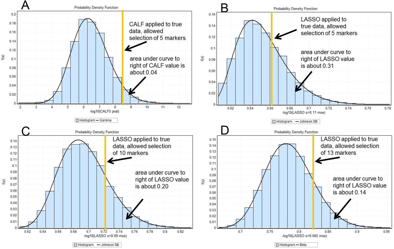
The surpass rates for the algorithms. (A) For the given binary classification problem, CALF with five markers is much less prone to a high surpass rate than LASSO with 5, 10, or 13 markers. The distributions depict the performance of CALF (metric −log10(pval)) applied to true data (orange line in A) vs those of CALF applied to 10000 trials with permuted data, then the analogous comparisons for three LASSO models (with metric −log10(mse)). The CALF5 sum yields Student p-value = 2.55E-09 for 40 NCs vs 35 Cs. The surpass rate is 0.038, customarily considered statistically significant.
The four solutions for true data follow.
CALF5 = +M040 +M135 -M123 +M070 -M086
LASSO5 = +0.433140 +0.018336*M027 +0.058302*M040 +0.001833*M070 −0.004697*M123 +0.027518*M135
LASSO10 = +0.4222400 +0.031884*M027 +0.092007*M040 +0.000846*M044 +0.001874*M062 +0.024605*M070 +0.000505*M079-0.012927*M086 +0.000185*M111-0.032877*M123 +0.044539*M135
LASSO13 = 0.392479 +0.042108*M027 +0.127132*M040 +0.0282959*M044 +0.008755*M062 +0.057780*M070 +0.004452*M073 +0.018423*M079 −0.055934*M086 +0.021428*M111-0.065415*M123-0.013102*M127 +0.006901*M132 +0.061733*M135
The CALF5 markers (yellow) generally appear in the LASSO solutions with the same signs.
Consistency of marker selection
To estimate the consistency of CALF5 choices over subsets of true date, we randomly selected ~90% subsets (so 36 of 40 NCs and 29 of 32 Cs) 10000 times. The numbers of times a marker was chosen with a particular sign are shown in Figure 4.

Counts of times markers were chosen with particular signs in CALF5 solutions of 10000 ~90% random subsets of NC and C subjects. Minimum shown = 336. All other marker’s counts <= 281. The bars show the above five markers used in CALF5 applied to 100% of true data are indeed far more popular than all other markers.
Decoding the above labels into actual marker labels7 yields the (unpublished) sum:

Each of the five selected markers has multiple functions described in its literature. However, all five are connected to immune functions as follows: MMP7 = Matrix Metalloproteinase-7 (activate innate immunity, proteolytic release of TNF from macrophages); MDA-LDL = Malondialdehyde-Modified Low-Density Lipoprotein (initiate pro-inflammatory response); MMP1 = Matrix Metalloproteinase-1 (neuroinflammation, disrupt BBB, demyelination, damage axons/neurons); TSH (B form is detected) = Thyroid-Stimulating Hormone (component of hypothalamus-pituitary-thyroid axis); and CXCL10 = C-X-C motif chemokine ligand 10 (activates monocyte, natural killer and T-cell migration). The mutual functions require further inquiry.
Cross validation
Upon application of CALF5 10000 times to a random choice of 4 NCs and 3 Cs (~10% subsets) the average AUC was 0.872 (SD = 0.132). Thus, the canonical CALF5 solution for 100% of true data well classifies many random ~10% subsets of true data into NC and C.
Cross validation requires computing a classifier from a random kept set of subjects (such as ~90% of controls and ~90% of cases) and applying each solution to the complementary subset. Doing so with the CALF program 10000 times yields observed AUC values for the unkept with average = 0.74 and SD = 0.16.
Additional regression methods applied to the same data
As described in Supplement 3, the same example was examined by the following eight classifier construction methods: two types of Logistic Regression; Stochastic Gradient Descent; Random Forest; a linear Support Vector Machine; KNN; GaussianNB; and a Decision Tree. Using selected or default parameters in limited ranges did not in any of the methods appear to offer reliable classification. Details including some parameter values are in Supplement 3.
Binary CALF optimizing AUC
Binary CALF can be configured to optimize AUC instead of pval as it selects markers and weights. Optimizing AUC or optimizing pval generally results in similar but not necessarily identical solutions. If optimizing AUC, then of course AUC improves (or CALF terminates) with every selection of a marker to add to the sum. During such selections, pval might or might not always improve.
Nonbinary targets for CALF—an example
All of the above addresses control vs case problems, that is, a target vector of binary values such as controls = 0 and cases = 1. Next is presentation of a nonbinary version of CALF that approximates by Pearson correlation target vectors that are nonbinary. Bioinformaticians will readily understand the goals and methods. The data matrix is in Supplement 4.
Monocytes are potentially useful prodromal indicators of risk of transition to schizophrenia.9 Using NAPLS data for 132 leukocytic miRNAs, we considered for 24 unaffected comparison subjects the problem of modeling from miRNAs the percentage by flow cytometry of monocytes in blood plasma. In other words, is there a deconvoluting leukocytic miRNA signature for monocytes?
The observed monocyte proportion among leukocytes was 0.20% to 1.20%; 18 of the 24 target values had only one digit of accuracy. Nonetheless, CALF was applied with an upper limit of 8 (of 132) markers; LASSO was applied (parameter s = 0.029) to yield a choice of 8 markers for the true data; also, Ridge was applied using all 132 markers (hence 132 real valued weights).
The CALF solution with eight markers (in order of CALF selection) and eight +1 weights is
CALF8 = +M081 +M034 -M090 +M128 +M067 -M075 -M049 +M127
The LASSO solution with intercept, eight selected markers (in order of decreasing weight magnitude), and eight real number weights is obtainable with parameter s=0.029.
LASSO8 = 0.440257927 +0.074811876*M081 +0.044522064*M034 +0.01966334*M118 - 0.014672181*M027 +0.008050587*M021 −0.003636177*M090 +0.001596755*M128 - 0.000152928*M035
Note that the four markers appearing both solutions (yellow) have weights of the same signs.
All three methods were tested for survival of permutations, meaning randomly permuting the 24 target entries and reapplying the three algorithms to the pseudo data 10000 times, exactly as though the pseudo data were the true data. For CALF with correlation = metric, the true correlation = 0.93 was exceeded by chance a total of 420 times, implying surpass rate of (420+1)/10001 = ~0.042 (Figure 5). By contrast, permutations of target entries with LASSO and Ridge, both using mse as a metric, resulted in surpass rates worse than the customary threshold 0.05. Note that correlations and mse were superior with CALF8. If more markers (smaller s parameter) are allowed, surpass rates for LASSO and Ridge become worse.

The correlation of the CALF8 approximation with the true target is 0.93. If the target vector is randomly permuted 10000 times, this histogram of bins of correlations (each 0.02 wide) and their frequencies is the result. The correlations of the CALF solution with the target is 0.93, yielding a surpass rate = 0.0420 = area under the curve to the right of the orange line (total area under curve = sum of shown frequencies = 1.00). This 0.0420 is < than the customary level of significance = 0.05 and much better than the surpass rates for LASSO and Ridge (Table 2).
Larger data matrices
Assays of DNA methylation in blood cell types yield frequencies of methylation marks as real numbers in [0, 1] for many thousands of positions in the genomes of patients and controls. Usually the work is on finding sets of marks that individually seem to distinguish the two groups. However, in preliminary experiments with ~22000 marks from 82 controls and 52 cases, running on a laptop (up to 3.6 GHz), CALF on all of true data yielded choices of marks to be used in an approximation of binary phenotype in a few tens of seconds. For limits L = 5, 10, 15, or 20 marks, CALF optimization of pval required about 27+6L seconds; for AUC optimization, 21+4L seconds. This observation suggests CALF with permutations parallelized on a large cluster could be feasible for larger data matrices.
Discussion
CALF deterministically seeks a coarse sum of a few markers to optimize a metric. Since the method and metric differ from those of LASSO, it is expected that performances on examples will differ.
Tested by permutations (described in Supplement 1), a CALF solution might provide a good classifier (binary) or correlation (nonbinary), but, as a greedy algorithm, it is not guaranteed to find the best choice of all possible markers weights to use. In fact, a simple example in Supplement 5 shows that its greedy approach fails to avoid entrapment in a local optimum and cannot for that example reach a global optimum.
The goal of CALF is discovery of a network of collectively informative markers, not identification of a set of markers that are individually informative. We can do so despite the computational explosion of numbers of possible sets of subsets precisely because: (1) CALF grows small sets to larger sets deterministically and simply; and (2) randomization tests assure us (or not) that the quality of the final result cannot be reasonably explained by chance.


