

Abstract
How patterns in community diversity emerge is a long-standing question in ecology. Theories and experimental studies suggested that community diversity and interspecific interactions are interdependent. However, evidence from multitaxonomic, high-diversity ecological communities is lacking because of practical challenges in characterizing speciose communities and their interactions. Here, I analyzed time-varying causal interaction networks that were reconstructed using 1197 species, DNA-based ecological time series taken from experimental rice plots and empirical dynamic modeling, and show that species interaction capacity, namely, the sum of interaction strength that a single species gives and receives, underpins community diversity. As community diversity increases, the number of interactions increases exponentially but the mean species interaction capacity of a community becomes saturated, weakening interaction among species. These patterns are explicitly modeled with simple mathematical equations, based on which I propose the “interaction capacity hypothesis”, namely, that species interaction capacity and network connectance are proximate drivers of community diversity. Furthermore, I show that total DNA concentrations and temperature influence species interaction capacity and connectance nonlinearly, explaining a large proportion of diversity patterns observed in various systems. The interaction capacity hypothesis enables mechanistic explanations of community diversity, and how species interaction capacity is determined is a key question in ecology.
Introduction
How patterns in community diversity in nature emerge is one of the most challenging and longstanding questions in ecology (Gaston 2000). Community diversity, or species diversity, a surrogate of biodiversity that is most commonly focused on (Willig et al. 2003), is a collective consequence of community assembly. Among the community assembly processes, interspecific interactions, which contribute to the process of selection, play an important role in shaping community diversity, particularly at a local (i.e., small/short spatiotemporal) scale, and thus they have played a central role when devising theories of ecological communities (Vellend 2016), including modern coexistence theory (Chesson 2000), niche theory (Chase & Leibold 2003), plant-soil feedbacks (Comita et al. 2010; Mangan et al. 2010; Ushio et al. 2017), and many others. Understanding how interspecific interactions shape community diversity is key to understanding how patterns in an ecological community emerge in nature.
Theoretical studies and simple manipulative experiments have supported the view that interspecific interactions contribute to community diversity (Reynolds & Bruno 2013; Bairey et al. 2016; Ratzke et al. 2020). Nonlinear, state-dependent interspecific interactions have been shown to influence community diversity, composition and even dynamics (Reynolds & Bruno 2013; Bairey et al. 2016; Ushio et al. 2018a), and weak interactions are key to the maintenance of community diversity (Wootton & Emmerson 2005; Ratzke et al. 2020). However, while the evidence is compelling, whether and how interspecific interactions control diversity in a natural complex ecological community remain poorly understood. This is largely due to two difficulties: (1) the number of species and interspecific interactions examined in previous studies have been limited compared with those of a real high-diversity ecological community under field conditions, and (2) detecting causalities between interspecific interactions and diversity is not straightforward because manipulative experiments, a most effective strategy to detect causality, are not feasible when a large number of species and interactions are targeted under field conditions. Nonetheless, understanding the mechanism by which interspecific interactions drive community diversity in nature is necessary for predicting responses of ecological communities and their functions to the ongoing global climatic and anthropogenic threats (Aronson et al. 2014).
To overcome the previous limitations and examine the causal relationships between interspecific interactions and diversity of a specious community, I integrated quantitative environmental DNA monitoring and a nonlinear time series analysis, and found that the capacity of species for interspecific interactions underpins community diversity. Efficient water sampling, DNA extraction and quantitative MiSeq sequencing (Ushio 2019) overcame the first difficulty noted above: quantitative, highly diverse, multitaxonomic, daily, 122-day-long ecological time series were obtained from five experimental rice plots under field conditions. This extensive ecological time series was analyzed using a framework of nonlinear time series analysis, empirical dynamic modeling (EDM) (Sugihara et al. 2012; Ye et al. 2015a; Deyle et al. 2016), to overcome the second difficulty: EDM quantified fluctuating interaction strengths, reconstructed the time-varying interaction network of the ecological communities, and detected causal relationships between network properties and community diversity. Here, I look specifically at how interaction strengths change with community diversity, and how interspecific interactions and community diversity are causally coupled. Then, I derive a hypothesis that explains community diversity in various systems, which I call the “interaction capacity hypothesis”.
Experimental design and ecological community monitoring
Ecological time series were taken from five experimental rice plots established at the Center for Ecological Research, Kyoto University, Japan (Fig. 1a, Figure S1). Ecological communities were monitored by analyzing DNA in water samples taken from the rice plots using two types of filter cartridge (Ushio 2019). Daily monitoring during the rice growing season of 2017 (23 May to 22 September) resulted in 1220 water samples in total (5 plots × 2 filter types [ϕ 0.45 – μm and ϕ 0.22 – μm filters] × 122 days). Prokaryotes and eukaryotes (including fungi and animals) were analyzed by amplifying and sequencing 16S rRNA, 18S rRNA, ITS (for which DNAs extracted from ϕ 0.22 – μm filters were used), and mitochondrial COI regions (for which DNAs from ϕ 0.45-μm filters were used), respectively, using a quantitative MiSeq approach (Ushio 2019). Over 80 million reads were generated by four runs of MiSeq, and the sequences generated were then analyzed using the amplicon sequence variants (ASVs) method (Callahan et al. 2016). Among over 10000 ASVs detected, 1197 ASVs (equivalent to 1197 taxonomic units) were abundant, frequently detected and contained enough temporal information for subsequent time series analyses (see Methods, Figures S2 and S3).

a Workflow of the present study. b Mean DNA concentrations of the ecological communities in rice plots. Different colours indicate different superkingdoms. b Temporal patterns of the number of ASVs detected from each plot. Different symbols and colours indicate different rice plots.
Community dynamics and reconstruction of fluctuating interaction network
The total DNA concentrations increased late in the sampling period (Fig. 1b). In contrast, ASV diversity (a surrogate of species diversity in the present study) was highest in August and then decreased in September (Fig. 1c). Prokaryotes largely accounted for this pattern (Figure S3), which is not surprising given their higher diversity and abundance compared to the other taxa.
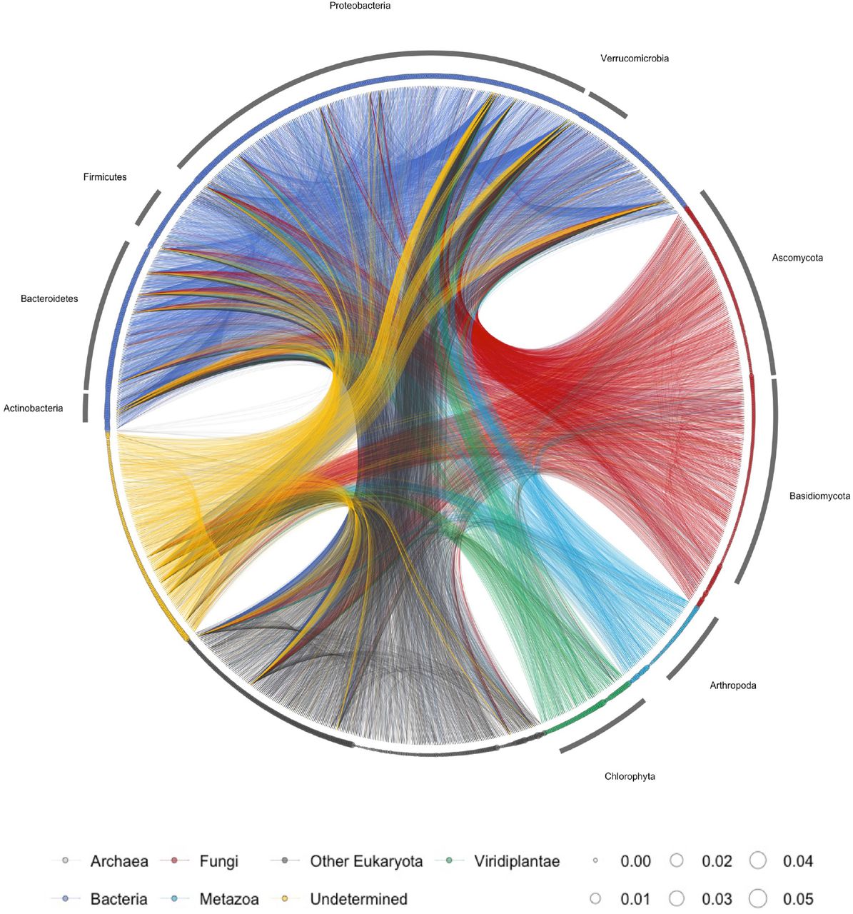
Fluctuating interaction networks were reconstructed using EDM, a time series analytical framework for nonlinear dynamics (Sugihara et al. 2012; Ye et al. 2015a; Deyle et al. 2016). In the analysis, I detected causally related ASV pairs using convergent cross mapping (CCM) (Sugihara et al. 2012), a causality test of EDM, and then quantified the interaction strengths by multivariate, regularized S-maps (Sugihara 1994; Deyle et al. 2016; Cenci et al. 2019). Figure 2 shows the reconstructed network of the detected interactions over the monitoring period (for the time-varying interaction networks, see Figure S4a). The properties of the ecological network changed over time (Figure S4a). For example, relatively dense interactions among community members in July and August (in Plot 1) disappeared by September. Interestingly, dynamic stability (Ushio et al. 2018a), an index that quantifies how fast the community bounces back from small perturbations, was almost always over 1, indicating unstable community dynamics (Figure S4b). This pattern may not be surprising because the rice plots were open systems under field conditions. Many community members could immigrate and emigrate, leading to inherently unstable dynamics.

Lines indicate causal influences between nodes, and line colours indicate causal taxa (e.g., blue lines indicate the causal influences from bacterial species to another species). The size of each node (circle) represents the relative DNA concentration of the ASV. Different colours of nodes indicate different taxa, as shown at the bottom. Note that, although interaction strengths were quantified at each time point, the information on the time-varying interactions are not shown in the network. The detailed, daily fluctuating interaction network will be available in https://github.com/ong8181/ecolnet-int-capacity as an animation.
Patterns emerging in the interaction networks
Properties of the interaction networks showed intriguing patterns. As ASV diversity increases, the mean interaction strength per link decreases (Fig. 3a; for mathematical definitions of network properties, see Methods), while the number of interactions in a community increases exponentially (Figure S5). This suggests that the total interaction strength that a species receives and gives cannot exceed a certain upper limit, which I call “interaction capacity”, even when ASV diversity and the number of interactions in a community increase. The availability of time and resources, which are required to interact with other species, are limited, and thus it is intuitively plausible to assume that there is a certain upper limit of interaction capacity. Indeed, the mean interaction capacity hit a plateau when ASV diversity was over 100 (Fig. 3b).

a–d Co-varying relationships (correlations) between ASV diversity and properties of the interaction network, i.e., the mean interaction strength (a), interaction capacity (b), connectance (c) and coefficients of variations in population dynamics (d). Interaction capacity is defined as the sum of absolute values of interaction strength that a species gives or receives. Dashed line in a indicates a converged value of mean interaction strength (≈ 0.03). e–h Relationships between interaction capacity, connectance, mean air temperature and total DNA concentrations. i–n Causal influences of air temperature and total DNA concentrations on connectance, interaction capacity and community diversity quantified by empirical dynamic modeling (EDM). Convergent cross mapping (CCM) was first applied to each pair, and then multivariate, regularized S-map was applied to quantify the causal influences. Red lines indiate significant nonlinear regressions by general additive model (GAM).
Another important property of the interaction networks, connectance, is also relatively constant as ASV diversity varies (Fig. 3c). Importantly, these patterns were not reproduced when the randomly shuffled version of the original time series was analyzed (Figure S6). In addition, this pattern of interaction strength per link decreasing and converging when the number of interactions and/or species is high is valid even at the species level (Figure S7a). These findings suggest that the original results may not have been experimental or statistical artifacts but rather may have emerged as consequences of empirical community assembly processes. Another intriguing pattern is that mean values of coefficients of variation (CV) of DNA concentrations, an index of realized temporal variability, decreases as a function of ASV diversity (Fig. 3d). This showed, for the first time, that the small temporal variability in species abundances observed in diverse plant communities (Tilman et al. 2006) is also valid even when all major cellular organisms are taken into account, and that there is a connection between community diversity and temporal dynamics in this system.
Community diversity and interaction capacity are directly coupled: the interaction capacity hypothesis
The implications of the patterns that emerged in the network properties can be explicitly shown by developing a simple mathematical model. Here I demonstrate that community diversity and interaction capacity are interdependent on each other. Since connectance, C, is defined as C = Nlink / S2, species diversity (species richness), S, can be simply represented as  , where Nlink indicates the total number of interactions in a community. Furthermore, Nlink can be decomposed into the mean interaction capacity at the community level (IC), defined as
  / S (see Methods), and the mean interaction strength per link, ISlink, as follows:

IC/ISlink is divided by 2 because each interaction strength is counted twice (for donor and receiver species). Therefore, S, C, IC and ISlink should satisfy the following relationship:

No system-specific assumption is used to derive Eqn. (2), and thus S, IC, ISlink and C should satisfy Eqn. (2) in any system and under any condition. Also, note that the four parameters are all interdependent, and thus a change in one parameter influences other parameters. When using the system-specific parameter value of converged ISlink in the present study (Fig. 3a), community diversity in the rice plots is described as follows:

This mathematical model indicates that species diversity can be predicted if we know how IC and C are determined in a community.
My ecological time series provides a unique opportunity to elucidate how interaction capacity (IC) and connectance (C) are determined under field conditions. In the analysis, I focused on two fundamental variables that are statistically independent of the network properties: air temperature and total DNA concentrations (an index of total abundance/biomass). Also, I focused on these because air temperature is an independent external driver of community dynamics and because total abundance could be an index of net ecosystem productivity or available energy in a system, which could be a potential driver of community diversity (e.g., Evans et al. 2005; Huston 2014). Correlation analysis shows that the interaction capacity is positively correlated with mean air temperature and total DNA concentration (Fig. 3e,f). Connectance is positively correlated with total DNA concentration, and is weakly correlated with mean air temperature (Fig. 3g,h).
Causal relationships between the properties were examined with CCM, and the results suggested that mean interaction capacity and connectance are causally influenced by mean air temperature and total DNA concentration (Figure S8). The S-map revealed that mean air temperature in general positively influenced interaction capacity and connectance, as indicated by mostly positive values along the gradient (Fig. 3i,j; values on the y-axis indicate how changes in temperature cause changes in interaction capacity or connectance). Temperature may influence many aspects of biological processes, e.g., physiological rates of individuals, and therefore, the influences of air temperature on interaction capacity and connectance may arise from the increased activities of individuals. Although temperature effects on connectance and mean interaction capacity at the community level were comparable, the net effects of temperature on diversity, that is, effects of temperature through its effects on interaction capacity and connectance, were consistently positive (Fig. 3k). This indicates that the positive influence of temperature on mean interaction capacity is stronger than that on connectance for shaping community diversity, which is consistent with Eqn. (2).
When total DNA concentration is low, its influence on connectance is variable (Fig. 3l). When total DNA concentration is high, however, total DNA concentration strongly and positively influences connectance, suggesting that denser populations should have higher connectance, probably because the greater population size may facilitate random encounters among individuals or species. On the other hand, the influences on interaction capacity are relatively small and variable (Fig. 3m). These results predict that total DNA concentrations (or abundance/biomass) over a certain threshold negatively influence diversity, which is indeed the case here (Fig. 3n).
Together, the results of EDM show that interaction capacity and connectance are influenced by temperature (T) and total DNA concentration (DNA), suggesting that species diversity, S, can be approximated using these two fundamental parameters as follows:

Although the influences of temperature and abundance (biomass or energy) on diversity have long been recognized in the literatures (e.g., Begon et al. 2005), this model, supported by empirical evidence, provides mechanistic explanations about how temperature and abundance control community diversity. Although the present study did not include other potentially important abiotic factors such as water pH and nutrient availability, the mechanisms of the influence of such factors may also be understood by considering their effects on interaction capacity and connectance. Because community diversity, interaction capacity and connectance are interdependent in any system and under any condition according to Eqn. (2), the influences of any biotic/abiotic factors on community diversity can be mechanistically explained and predicted if we can understand the influences of these factors on interaction capacity and connectance, a hypothesis which I call the “interaction capacity hypothesis”.
Predicting diversity of a natural ecological community
The simple mathematical model and the analyses of the extensive ecological time series reported here suggest that proximate drivers of community diversity are interaction capacity and con-nectance, and that the long-recognized patterns that temperature and total species abundance influence community diversity are underpinned by their influences on interaction capacity and connectance. In some cases, variable responses of community diversity to temperature and/or abundance might be observed because of the nonlinear influences of temperature and abundance on interaction capacity and connectance (Fig. 3i-n). Conversely, if the present results can be generalized to other systems, it should be possible to explain community diversity reasonably well by a nonlinear regression using temperature and total abundance. Indeed, this expectation was verified by analyzing datasets from diverse taxa and ecosystems (Masuda 2008; Sunagawa et al. 2015; Okazaki et al. 2017; Bahram et al. 2018; Okano et al. 2018; Sakamoto et al. 2018) that included information about diversity, temperature and an index of total species abundance or biomass. The simple, nonlinear regressions between diversity, temperature and abundance explained community diversity surprisingly well for the five aquatic data sets (Figure S9 and Supporting Information; adjusted R2 = 0.453 – 0.792), supporting the generality of the interaction capacity hypothesis.
The interaction capacity hypothesis provides quantitative and unique predictions about community diversity in nature. For example, everything else being equal, community diversity may increase with increasing temperature because of increased interaction capacity under warmer conditions (Fig. 4a, b). Similarly, community diversity will increase with increasing habitat heterogeneity because of decreased connectance (Fig. 4a, b). Thus, high diversity communities will exist under optimal environmental conditions (i.e., high interaction capacity) with spatially heterogeneous habitats (i.e., low connectance), such as those in tropical forests or soils with neutral pH (Fig. 4c, d). Furthermore, under such conditions, community dynamics will be stabilized because of the decreased interaction strengths (Figs. 3d, 4c; also see evidence from a recent experimental study, Ratzke et al. 2020). On the other hand, low-diversity communities will exist under extreme environmental conditions with spatially homogeneous habitats, such as deserts, because of decreased (or consumed) interaction capacity and increased connectance.

a Potential external drivers that contribute to the community diversity and network structure. b Mechanisms of community assembly. Extreme and optimal temperature would generally decrease and increase species interaction capacity, respectively. Spatial heterogeneity decreases connectance, which subsequently increases community diversity. c Outcomes of community diversity and dynamics. Extreme temperature and low spatial heterogeneity generate a community with low diversity, strong interaction strength and unstable dynamics. On the other hand, optimal temperature and high spatial heterogeneity generate a community with high diversity, weak interaction strength and stable community dynamics. d Examples of ecological communities (low-diversity versus high-diversity community) according to the potential external drivers and the interaction capacity hypothesis.
Future directions
Considering the interdependence between interaction capacity and community diversity, how interaction capacity is determined will be a central question in ecology. For example, interaction capacity may be influenced by energy and resources provided to a system, but it can also be influenced by species identity (i.e., species’ ecology, physiology and evolutional history; e.g., higher interaction capacities of prokaryotes than of eukaryotes; see Figure S7b). Incorporating species identity into the interaction capacity hypothesis would be an interesting direction for future studies.
In addition, abiotic factors can easily and explicitly be incorporated into the interaction capacity hypothesis. For example, if interaction capacity (or energy resources) is “consumed” to adapt to harsh environmental conditions, interaction capacity that can be used for interspecific interaction will decrease, which will consequently decrease community diversity. Lastly, applying the interaction capacity hypothesis to other systems such as gene expression, neural networks and even human networks should lead to fresh insights.
Conclusions
How patterns in community diversity emerge has been extensively studied by experimental and theoretical approaches, yet rarely examined for highly diverse, complex ecological communities. Using DNA-based, highly frequent, quantitative, extensive ecological time series and EDM, I present evidence that interaction capacity is a key to understanding and predicting community diversity. Connectance may also play an important role, because it determines how interaction capacity is divided into each interaction link. Interaction capacity is influenced by the total abundance and temperature, which can provide mechanistic explanations for many observed ecological patterns in nature. Expanding spatial and temporal scales and incorporating the other processes in community assembly (that is, speciation, dispersal and drift) (Vellend 2016) into the interaction capacity hypothesis will further deepen our understanding of community assembly processes, which will contribute to how we can predict, manage and conserve biodiversity and the resultant ecosystem functions in nature.
Methods
Experimental setting
Five artificial rice plots were established using small plastic containers (90 × 90 × 34.5 cm; 216 L total volume; Risu Kogyo, Kagamigahara, Japan) in an experimental field at the Center for Ecological Research, Kyoto University, in Otsu, Japan (34° 58’ 18” N, 135° 57’ 33” E). Sixteen Wagner pots (ϕ 174.6 × ϕ 160.4 × 197.5 mm; AsOne, Osaka, Japan) were filled with commercial soil, and three rice seedlings (var. Hinohikari) were planted in each pot on 23 May 2017 and then harvested on 22 September 2017 (122 days; Table S1). The rice growth data are being analyzed for different purposes and thus are not shown in this report. The containers (hereafter, “plots”) were filled with well water, and the ecological community was monitored by analyzing DNA in the well water (see following subsections).
Field monitoring of the ecological community
To monitor the ecological community, water samples were collected daily from the five rice plots. Approximately 200 ml of water in each rice plot was collected from each of the four corners of the plot using a 500-ml plastic bottle and taken to the laboratory within 30 minutes. Water samples were kept at 4°C during transport. The water was filtered using Sterivex™ filter cartridges (Merck Millipore, Darmstadt, Germany). Two types of filter cartridges were used to filter water samples: to detect microorganisms, ϕ 0.22-//m Sterivex™ (SVGV010RS) filters that included zirconia beads (for degradation of the microbial cell wall) were used (Ushio 2019), and to detect macroorganisms, ϕ 0.45-μm Sterivex™ (SVHV010RS) filters were used. Water in each plastic bottle was thoroughly mixed before filtration, and 30 ml and 100 ml aliquots of the water were filtered using ϕ 0.22-μm and ϕ 0.45-μm Sterivex™, respectively (slightly adjusted when the filters were clogged). After filtration, 2 ml of RNAlater™ solution (ThermoFisher Scientific, Waltham, Massachusetts, USA) were added to each filter cartridge to prevent DNA degradation during storage. In total, 1220 water samples (122 days × 2 filter types × 5 plots) were collected during the census term. In addition, 30 field-level negative controls, 32 PCR-level negative controls with or without the internal standard DNAs and 10 positive controls to monitor the potential DNA cross-contamination and degradation during the sample storage, transport, DNA extraction and library preparations were used. Visual inspections of the negative and positive control results indicated no serious DNA contaminations or degradation during analyses (Figure S2). Detailed information on the negative/positive controls are provided in Supplementary Information.
DNA extractions
DNA was extracted using a DNeasy® Blood & Tissue kit following a protocol described in my previous report (Ushio 2019). First, the 2 ml of RNAlater solution in each filter cartridge were removed from the outlet under vacuum using the QIAvac system (Qiagen, Hilden, Germany), followed by a further wash using 1 ml of MilliQ water. The MilliQ water was also removed from the outlet using the QIAvac. Then, Proteinase K solution (20 μl), PBS (220 μl) and buffer AL (200 μl) were mixed, and 440 μ1 of the mixture was added to each filter cartridge. The materials on the cartridge filters were subjected to cell lysis by incubating the filters on a rotary shaker (15 rpm; DNA oven HI380R, Kurabo, Osaka, Japan) at 56°C for 10 min. After cell lysis, filter cartridges were vigorously shaken (with zirconia beads inside the filter cartridges for 0.22 – μm cartridge filters) for 180 sec (3200 rpm; VM-96A, AS ONE, Osaka, Japan). The bead-beating process was omitted for 0.45-//m cartridge filters. The incubated and lysed mixture was transferred into a new 2-ml tube from the inlet (not the outlet) of the filter cartridge by centrifugation (3500 g for 1 min). Zirconia beads were removed by collecting the supernatant of the incubated mixture after the centrifugation. The collected DNA was purified using a DNeasy® Blood & Tissue kit following the manufacturer’s protocol. After the purification, DNA was eluted using 100 μl of the supplied elution buffer. Eluted DNA samples were stored at −20° C until further processing.
Library preparation
Prior to the library preparation, work spaces and equipment were sterilized. Filtered pipet tips were used, and pre-PCR and post-PCR samples were separated to safeguard against cross-contamination. PCR-level negative controls (i.e., with and without internal standard DNAs) were employed for each MiSeq run to monitor contamination during the experiments.
Details of the library preparation process are described in Supplementary Information. Briefly, the first-round PCR (first PCR) was carried out with the internal standard DNAs to amplify metabarcoding regions of prokaryotes (515F-806R primers) (Bates et al. 2011), eukaryotes (Euk_1391f and EukBr primers) (Amaral-Zettler et al. 2009), fungi (ITS1-F-KYO1 and ITS2-KYO2) (Toju et al. 2012) and animals (mostly invertebrates in the present study) (mlCOIintF and HCO2198 primers) (Folmer et al. 1994; Leray et al. 2013). After the purifications of the triplicate 1st PCR products, the second-round PCR (second PCR) was carried out to append indices for different templates (samples) for massively parallel sequencing with MiSeq. Twenty microliters of the indexed second PCR products were mixed, the combined library was purified, and targetsized DNA of the purified library was excised and quantified. The double-stranded DNA concentration of the library was then adjusted using MilliQ water and the DNA was applied to the MiSeq (Illumina, San Diego, CA, USA).
Sequence processing: Amplicon sequence variant (ASV) approach
The raw MiSeq data were converted into FASTQ files using the bcl2fastq program provided by Illumina (bcl2fastq v2.18). The FASTQ files were then demultiplexed using the command implemented in Claident (http://www.claident.org) (Tanabe & Toju 2013). I adopted this process rather than using FASTQ files demultiplexed by the Illumina MiSeq default program in order to remove sequences whose 8-mer index positions included nucleotides with low quality scores (i.e., Q-score < 30).
Demultiplexed FASTQ files were analyzed using the Amplicon Sequence Variant (ASV) method implemented in the DADA2 (v1.11.5) (Callahan et al. 2016) package of R. First, the primers were removed using the external software cutadapt v2.6 (Martin 2011). Next, sequences were filtered for quality using the DADA2::filterAndTrim() function, and rates were learned using DADA2::learnErrors() function (MAX_CONSIST option was set as 20). Then, sequences were dereplicated, error-corrected, and merged to produce an ASV-sample matrix. Chimeric sequences were removed using the DADA2::removeBimeraDenove() function.
Taxonomic identification was performed for ASVs inferred using DADA2 based on the query-centric auto-k-nearest-neighbor (QCauto) method (Tanabe & Toju 2013) and subsequent taxonomic assignment with the lowest common ancestor algorithm (Huson et al. 2007) using “overall_class” and “overall_genus” database and clidentseq, classigntax and clmergeassign commands implemented in Claident v0.2.2019.05.10. I chose this approach because the QCauto method assigns taxa in a more conservative way (i.e., low possibility of false taxa assignment) than other methods. Because the QCauto method requires at least two sequences from a single microbial taxon, only internal standard DNAs were separately identified using BLAST (Camacho et al. 2009).
After the taxa assignment, sequence performance was carefully examined using rarefaction curves, detected reads from PCR and field negative controls (Figure S2 and Supplementary Information). The results suggested that the sequencing captured most of the diversity and there were low levels of contamination during the monitoring, DNA extractions, library preparations and sequencing.
Estimations of DNA copy numbers
For all analyses in this subsection, the free statistical environment R 3.6.1 was used (R Core Team 2019). The procedure used to estimate DNA copy numbers consisted of two parts, following previous studies (Ushio et al. 2018b; Ushio 2019): (1) linear regression analysis to examine the relationship between sequence reads and the copy numbers of the internal standard DNAs for each sample, and (2) the conversion of sequence reads of non-standard DNAs to estimate the copy numbers using the result of the linear regression for each sample. Linear regressions were used to examine how many sequence reads were generated from one DNA copy through the library preparation process. Note that a linear regression analysis between sequence reads and standard DNAs was performed for each sample and the intercept was set as zero. The regression equation was: MiSeq sequence reads = regression slope × the number of standard DNA copies [/μl].
The sequence reads of non-standard DNAs were converted to copy numbers using sample-specific regression slopes estimated using the above regression analysis. The number of non-standard DNA copies was estimated by dividing the number of MiSeq sequence reads by the value of a sample-specific regression slope (i.e., the number of DNA copies = MiSeq sequence reads/regression slope). A previous study demonstrated that these procedures provide a reasonable estimate of DNA copy numbers using high-throughput sequencing (Ushio et al. 2018b).
After the conversion to DNA copy number, ASVs with low DNA concentrations were excluded because their copy numbers are not sufficiently reliable. Also, ASVs with low entropy (information contained in the time series) were excluded because reliable analyses of EDM require a sufficient amount of temporal information in the time series.
Empirical dynamic modeling: Convergent cross mapping (CCM)
The reconstruction of the original dynamics using time-lagged coordinates is known as State Space Reconstruction (SSR) (Takens 1981; Deyle & Sugihara 2011) and is useful when one wants to understand complex dynamics. Recently developed tools for nonlinear time series analysis called “Empirical Dynamic Modeling (EDM)”, which were specifically designed to analyze state-dependent behavior of dynamic systems, are rooted in SSR (Sugihara et al. 2012; Ye et al. 2015a; Deyle et al. 2016; Ushio et al. 2018a). These methods do not assume any set of equations governing the system, and thus are suitable for analyzing complex systems, for which it is often difficult to make reasonable a priori assumptions about their underlying mechanisms. Instead of assuming a set of specific equations, EDM recovers the dynamics directly from time series data, and is thus particularly useful for forecasting ecological time series, which are otherwise often difficult to forecast.
To detect causation between species detected by the DNA analysis, I used convergent cross mapping (CCM) (Sugihara et al. 2012; Osada et al. unpublished). An important consequence of the SSR theorems is that if two variables are part of the same dynamical system, then the reconstructed state spaces of the two variables will topologically represent the same attractor (with a one-to-one mapping between reconstructed attractors). Therefore, it is possible to predict the current state of a variable using time lags of another variable. We can look for the signature of a causal variable in the time series of an effect variable by testing whether there is a correspondence between their reconstructed state spaces (i.e., cross mapping). This cross-map technique can be used to detect causation between variables. Cross-map skill can be evaluated by either a correlation coefficient (p), or mean absolute error (MAE) or root mean square error (RMSE) between observed values and predictions by cross mapping.
In the present study, cross mapping from one variable to another was performed using simplex projection (Sugihara & May 1990). How many time lags are taken in SSR (i.e, optimal embedding dimension; E) is determined by simplex projection using RMSE as an index of forecasting skill. More detailed algorithms about simplex projection and cross mapping can be found in previous reports (Sugihara & May 1990; Sugihara et al. 2012).
When the causal relationships between network properties were examined, I considered the interaction time lag between the network properties. This can be done by using “lagged CCM” (Ye et al. 2015b). For normal CCM, correspondence between reconstructed state space (i.e., cross-mapping) is checked using the same time point. In other words, information embedded in an effect time series at time t may be used to predict the state of a potential causal time series at time t. This idea can easily be extended to examine time-delayed influence between time series by asking the following question: is it possible to predict the state of a potential causal time series at time t-tp (tp is a time delay) by using information embedded in an effect time series at time t? Ye et al. (2015b) showed that lagged CCM is effective for determining the effective time delay between variables. In the present study, I examined the time delay of the effects from 0 to 14 days. When examining species interaction in the rice plots, the time delay of the interactions was fixed as −1 in order to avoid extremely large computational costs (i.e., 1197 × 1197 CCMs must be performed for each tp).
The significance of CCM is judged by comparing convergence in the cross-map skill of Fourier surrogates and original time series. More specifically, first, 1000 surrogate time series for one original time series are generated. Second, the convergence of the cross-map skill is calculated for these 1000 surrogate time series and the original time series. Specifically, the convergence of the cross-map skill (measured by ΔRMSE in the present study) is calculated as the cross-map skill at the maximum library length minus that at the minimum library length (Sugihara et al. 2012; Osadda et al. unpublished). Based on consideration of a large number of CCMs among 1197 DNA species, I used P = 0.005 as threshold. For CCMs among the network properties, I used P = 0.05, a more commonly used threshold.
Empirical dynamic modeling: Multivariate, regularized S-map method
The multivariate S-map (sequential locally weighted global linear map) method allows quantifications of dynamic (i.e., time-varying) interactions (Sugihara 1994; Deyle et al. 2016). Consider a system that has E different interacting variables, and assume that the state space at time t is given by x(t) = {x1(t),x2(t), …,xE(t)}. For each target time point t*, the S-map method produces a local linear model that predicts the future value x1(t* +p) from the multivariate reconstructed state space vector x(t*). That is,
 where
where  is a predicted value of x1 at time t* + p, and IS0 is an intercept of the linear model. The linear model is fit to the other vectors in the state space. However, points that are close to the target point, x(t*), are given greater weighting (i.e., locally weighted linear regression). Note that the model is calculated separately for each time point, t. As recently shown, ISj, the coefficients of the local linear model, are a proxy for the interaction strength between variables (Deyle et al. 2016). In the same way as with simplex projection and CCM, the performance of the multivariate S-map was also measured by RMSE (or a correlation coefficient, ρ) between observed and predicted values by the S-map (i.e., leave-one-out cross validation). In the present study, to reduce the possibility of overestimation and to improve forecasting skill, a regularized version of multivariate S-map was used (Cenci et al. 2019).
Calculations of properties of the interaction network
Properties of the reconstructed interaction network calculated include: ASV diversity, the number of interactions, connectance, mean interaction strength (IS) per link, mean interaction capacity, dynamic stability and coefficient of variation (CV) in population dynamics. Next, I give the definitions of the properties.
ASV diversity and the number of interactions are the number of ASVs present in a community and the number of interactions among ASVs present in a community, respectively. Connectance, C, is defined as C = Nlink / S2, where S and Nlink indicate the number of species and the number of interactions (links) in a community, respectively. Mean interaction strength per link, ISlink, was calculated as follows:
 , where ISi→j indicates an S-map coefficient from ith species to jth species. Note that I took the absolute value of the S-map coefficient when calculating ESlink. Mean interaction capacity, IC, was calculated as follows:

Species interaction capacity is defined as the sum of interactions that a single species gives and receives, and mean interaction capacity of a community is the averaged species interaction capacity. Dynamic stability of the community dynamics was calculated as the absolute value of the dominant eigenvalue of the interaction matrix (i.e., local Lyapunov exponent) as described in a previous study (Ushio et al. 2018a). CV of the community dynamics at time t was calculated as follows:
 , where
  and
and  indicate the standard deviation and mean value of the abundance of species i from time t-3 to t + 3, respectively (i.e., one-week time window). S(t) is the number of ASVs at time t.
Empirical dynamic modeling: Random shuffle surrogate test
To test whether the patterns generated (e.g., in Fig. 3) are statistical artifacts, I did a random shuffle surrogate test. In the test, the original time series were randomly shuffled within a plot using the rEDM::make_surrogate_shuffle() function in the rEDM package (Ye et al. 2015a, 2018) of R. Then, the same number of causal pairs was randomly assigned in a randomly shuffled ecological community. The regularized, multivariate S-map and subsequent analyses of the network properties (all identical to the original analyses) were applied to the randomly shuffled time series.
Meta-analysis of biodiversity, temperature and abundance
To validate my hypothesis that the diversity is determined by interaction capacity and connectance, and that they are influenced by temperature and total organism abundance, I compiled published data from various ecosystems. The collected data include two global datasets and four local datasets collected in Japan: (1) global ocean microbes (Sunagawa et al. 2015), (2) global soil microbes (Bahram et al. 2018), (3) fish from a coastal ecosystem (Masuda 2008), (4) prokaryotes from freshwater lake ecosystems (Okazaki et al. 2017), (5) zooplankton from a freshwater lake ecosystem (Sakamoto et al. 2018) and (6) benthic macroinvertebrates from freshwater tributary lagoon ecosystems (Okano et al. 2018). Because the influences of temperature and total species abundance/biomass on community diversity (or interaction capacity and connectance) are likely to be nonlinear, I adopted a general additive model (Wood 2004) as follows:
 where S, T, A and S() indicate species diversity (or OTU diversity), temperature, an index of total species abundance (or biomass) and a smoothing term, respectively. The relationships between diversity, temperature and total abundance were analyzed using the model described in the main text. GAM was performed using the “mgcv” package of R (Wood 2004).
Data analyzed in the meta-analysis were collected from the publications or official websites [Sunagawa et al. (2015); (Sakamoto et al. 2018), or provided by the authors of the original publications (Masuda 2008; Okazaki et al. 2017; Bahram et al. 2018;Okano et al. 2018). Therefore, raw data for the meta-analysis are available from the original publications, or upon reasonable requests to corresponding authors of the original publications.
Computation and results visualization
Simplex projection, S-map and CCM were performed using “rEDM” package (version 0.7.5) (Ye et al. 2015a, 2018), with results visualized using “ggplot2” (Wickham 2009). Data were analyzed in the free statistical environment R3.6.1 (R Core Team 2019).
Data and code availability
All scripts used in the present study will be available in Github (https://github.com/ong8181/ecolnet-int-capacity). Sequence data are deposited in DDBJ Sequence Read Archives (DRA) (DRA accession number = DRA009658, DRA009659, DRA009660 and DRA009661), which will be publicly available after the formal acceptance of the preprint.
Funding information
This research was supported by PRESTO (JPMJPR16O2) from the Japan Science and Technology Agency (JST) and the Hakubi Project in Kyoto University.
Competing interests
The author declares no competing interests.
Author Contributions
M.U. conceived the idea, designed research, collected data, analyzed DNA sequences and ecological time series, performed meta-analysis and wrote the manuscript.
Acknowledgements
I thank Asako Kawai for the assistance in field monitoring and DNA library preparations, Akira Matsumoto, Satoru Yonezawa and Satomi Yoshinami for assistance in the monitoring setup and field monitoring, Yutaka Osada for advice and discussion on empirical dynamic modeling, Takeshi Miki, Erik A. Hobbie, Masahiro Ryo and Hao Ye for comments on the manuscript, and Ai Matsuda for help in the figure editing. I also thank Mohammad Bahram, Yukiko Goda, Jun-ichi Okano, Yusuke Okazaki, Noboru Okuda, and Atsuya Shibata for providing the data set for the metaanalysis.
Footnotes
Minor errors included in Figure 1 have been corrected.


