GWAS of three molecular traits highlights core genes and pathways alongside a highly polygenic background

Summary

Genome-wide association studies (GWAS) have been used to study the genetic basis of a wide variety of complex diseases and other traits. However, for most traits it remains difficult to interpret what genes and biological processes are impacted by the top hits. Here, as a contrast, we describe UK Biobank GWAS results for three molecular traits—urate, IGF-1, and testosterone—that are biologically simpler than most diseases, and for which we know a great deal in advance about the core genes and pathways. Unlike most GWAS of complex traits, for all three traits we find that most top hits are readily interpretable. We observe huge enrichment of significant signals near genes involved in the relevant biosynthesis, transport, or signaling pathways. We show how GWAS data illuminate the biology of variation in each trait, including insights into differences in testosterone regulation between females and males. Meanwhile, in other respects the results are reminiscent of GWAS for more-complex traits. In particular, even these molecular traits are highly polygenic, with most of the variance coming not from core genes, but from thousands to tens of thousands of variants spread across most of the genome. Given that diseases are often impacted by many distinct biological processes, including these three, our results help to illustrate why so many variants can affect risk for any given disease.

Introduction

One of the central goals of genetics is to understand how genetic variation (and other sources of variation) map into phenotypic variation. Understanding the mapping from genotype to phenotype is at the heart of fields as diverse as medical genetics, evolutionary biology, behavioral genetics, and plant and animal breeding. During the last fifteen years, genome-wide association studies (GWAS) have been used to investigate the genetic basis of a wide variety of human complex traits and diseases [1].

This work has revealed that most traits are highly polygenic: the top hits contribute only a small fraction of the total heritability, and the bulk of the heritability is due to huge numbers of variants of small effect spread widely across the genome. In a pair of recent papers, we argued that there is a need for new conceptual models to make sense of the architecture of complex traits [2, 3]. How should we understand the observation that so many variants, spread widely across the genome, contribute to any given trait?

As a conceptual framework, we proposed a model in which there is a set of “core” genes, defined as genes with a direct effect on the trait that is not mediated through regulation of other genes. Meanwhile, other genes that are expressed in trait-relevant cell types are referred to as “peripheral” genes, and can matter if they affect the expression of core genes. We proposed that most trait variance is due to huge numbers of weak trans-regulatory effects from SNPs at peripheral genes. In what we referred to as the “omnigenic” extreme, potentially any gene expressed in trait-relevant cell types could affect the trait through small effects on core gene expression (albeit the distribution of peripheral gene effect sizes would be centered on zero, and in practice not all genes have regulatory variants).

Thus far it has been difficult to test this model because for most diseases and other traits we know little in advance about which genes are likely to be directly involved in disease biology. Furthermore, we still have highly incomplete information about cellular regulatory networks. Here we study in detail three traits that are unusually tractable to gain insights into the roles of core genes and the polygenic background.

GWAS of model traits: three vignettes

We investigate the genetic architecture of three molecular traits: serum urate, IGF-1, and testosterone levels. For each of these traits we know a great deal in advance about the key organs, biological processes and genes that might control these traits. This stands in contrast to many of the traits that have been studied extensively with GWAS, such as schizophrenia [4] (which is poorly understood at the molecular level) or height [5] (where we understand more of the underlying biology, but for which a large number of different biological processes contribute variance).

As described in more detail below, we performed GWAS for each of these traits in around 300,000 white British individuals from the UK Biobank [6]. For all three traits many of the top hits are highly interpretable–a marked difference from GWAS of typical disease traits. While these three molecular traits highlight different types of lead genes and molecular processes, they also have strikingly similar overall architectures: the top hits are generally close to genes with known biological relevance to the trait in question, and all three traits show strong enrichment in relevant gene sets. Most of the top hits would be considered core genes (or occasionally master regulators) in the sense of Liu et al (2019) [3].

At the same time however, the lead genes and pathways explain only a modest fraction of the heritability. Aside from one major-effect variant for urate, the lead pathways explain ~10% of the SNP heritability. Instead, most of the heritability is due to a highly polygenic background, which we conservatively estimate as being due to around 10,000 causal variants per trait.

In summary, these three molecular traits provide points of both contrast and similarity to the architectures of disease phenotypes. From one point of view they are clearly simpler, successfully identifying known biological processes to an extent that is highly unusual for disease GWAS. At the same time, the hits that “make sense” sit on a hugely polygenic background that is reminiscent of GWAS for more-complex traits. Lastly, many disease traits are themselves affected by molecular traits such as the three considered here. Given that each of these endophenotypes is already highly polygenic, we can clearly expect that any disease phenotype that depends on many such traits will itself be massively polygenic.

Results

Our analyses make use of GWAS results that we reported previously on blood and urine biomarkers [7], with minor modifications. In the present paper we report four primary GWAS analyses: urate, IGF-1, and testosterone in females and males separately. Prior to each GWAS, we adjusted the phenotypes by regressing the measured phenotypes against age, sex (urate and IGF-1 only), self-reported ethnicity, the top 40 principal components of genotype, assessment center and month of assessment, sample dilution and processing batch, as well as relevant pairwise interactions of these variables (Methods).

We then performed GWAS on the phenotype residuals in White British participants. For the GWAS we used variants imputed using the Haplotype Reference Consortium with MAF > 0.1% and INFO > 0.3 (Methods), yielding a total of 16M variants. The final sample sizes were 318,526 for urate, 317,114 for IGF-1, 142,778 for female testosterone, and 146,339 for male testosterone. One important goal of our paper is to identify the genes and pathways that contribute most to variation in each trait. For gene set-enrichment analyses, we annotated gene sets using a combination of KEGG [8] and previous trait-specific reviews, as noted in the text. We considered a gene to be “close” to a genome-wide significant signal if it was within 100kb of at least one lead SNP with p<5e-8. The annotations of lead signals on the Manhattan plots were generally guided by identifying nearby genes within the above-described enriched gene sets, or occasionally other strong nearby candidates.

Genetics of serum urate levels

Urate is a small molecule (C₅H₄N₄O₃) that arises as a metabolic by-product of purine metabolism and is released into the blood serum. Serum urate levels are regulated by the kidneys, where a set of transporters shuttle urate between the blood and urine; excess urate is excreted via urine. Urate is used as a clinical biomarker due to its associations with several diseases. Excessively high levels of urate can result in the formation of needle-like crystals of urate in the joints, a condition known as gout. High urate levels are also linked to diabetes, cardiovascular disease and kidney stones.

The genetics of urate have been examined previously by several groups [12, 13, 14, 15, 16, 17] and recently reviewed by [18]. The three strongest signals for urate lie in solute carrier genes: SLC2A9, ABCG2, and SLC22A11/SLC22A12. A recent trans-ancestry analysis of 457k individuals identified 183 genome-wide significant loci [17]; their primary analysis did not include UK Biobank. Among other results, this study highlighted genetic correlations of urate with gout and various metabolic traits; tissue enrichment signals in kidney and liver; and genetic signals at the master regulators for kidney and liver development HNF1A and HNF4A.

Performing GWAS of urate in the UK Biobank data set, we identified 222 independent genome-wide significant signals, summarized in Figure 1A (further details in Supplemental Data 1). Remarkably, six of the top ten signals are located within 100kb of a urate solute transport gene. A recent review identified ten genes that are involved in urate solute transport in the kidneys [9, 10]; in addition to the six transporters with extremely strong signals, two additional transporters have weaker, yet still genome-wide significant signals (Figure 1B). Hence, GWAS highlights eight out of ten annotated urate transporters, though some transporters were originally identified using early GWAS for urate levels. The two genes in the pathway that do not have hits (SMCT1 and SMCT2; also known as SLC5A8 and SLC5A12) do not directly transport urate, but instead transport mono-carboxylate substrates for URAT1 to increase reabsorption rate [19] and thus may be less direct regulators of urate levels.

Figure 1: Genetic basis of serum urate variation.

A. Genome wide associations with serum urate levels in the UK Biobank. Candidate genes that may drive the top signals are indicated; in most cases in the paper the indicated genes are within 100kb of the corresponding lead SNPs. B. Eight out of ten genes that were previously annotated as being involved in urate transport [9, 10] are within 100kb of a genome-wide significant signal. The signal at MCT9 is excluded from figure and enrichment due to its uncertain position in the pathway [11]. C. Urate heritability is highly enriched in kidney regulatory regions compared to the genome-wide background (analysis using stratified LD Score regression). Other tissues show little or no enrichment after removing regions that are active in kidney. See Figure S1 for the uncorrected analysis.

Among the other top hits, five are close to transcription factors involved in kidney and liver development (HNF4G, HNF1A, HNF4A, HLF and MAF). These are not part of a globally enriched gene set, but recent functional work has shown that the associated missense variant in HNF4A results in differential regulation of the urate solute carrier ABCG2 [17], while the MAF association has been shown to regulate SLC5A8 [20]. Finally, two other loci show large signals: a missense variant in INHBC, a TGF-family hormone, and a variant in/near GCKR, a glucose-enzyme regulator. Both variants have highly pleiotropic effects on many biomarkers, although the mechanisms pertaining to urate levels are unclear.

While most of the top hits are likely associated with kidney function, we wanted to test whether other tissues contribute to the overall heritability (Figure 1C). To this end, we used stratified LD Score regression to estimate the polygenic contribution of regulatory regions in ten previously defined tissue groupings [21]. Serum urate heritability was most-highly enriched in kidney regulatory regions (29-fold compared to the genome-wide average SNP, p = 1.9e-13), while other cell types were enriched around 8-fold (Figure S1; see also [17]). We hypothesized that the enrichment for other tissues might be driven by elements shared between kidney and other cell types. Indeed, when we removed active kidney regions from the regulatory annotations for other tissues, this eliminated most of the signal found in other cell types (Figure 1C). Thus, our analysis supports the inference that most serum urate heritability is driven by kidney regulatory variation.

Finally, while these signals emphasize the role of the kidneys in setting urate levels, we wanted to test specifically for a role of urate synthesis (similar to recent work on glycine [22]). The urate molecule is the final step of purine breakdown; most purines are present in tri-and monophosphates of adenosine and guanosine, where they act as signaling molecules, energy sources for cells, and nucleic acid precursors. The breakdown pathways are well known, including the genes that catalyze these steps (Figure 2A).

Figure 2: Modest enrichment of signals among genes involved in urate biosynthesis.

A. Urate is a byproduct of the purine biosynthesis pathway. The urate component of each molecule is highlighted B. The same pathway indicating genes that catalyze each step. Genes with a genome-wide significant signal within 100kb are indicated in red; numbers in grey indicate the presence of additional genes without signals. Pathway adapted from KEGG.

Overall we found that genes in the urate metabolic pathway show a modest enrichment for GWAS hits relative to all annotated, protein coding genes as a background (2.1-fold, p = 0.017; Figure 2B). XDH, which catalyzes the last step of urate synthesis has an adjacent GWAS hit, as do a number of upstream regulators of urate synthesis. Nonetheless, the overall level of signal in the synthesis pathway is modest compared to that seen for kidney urate transporters, suggesting that synthesis, while it plays a role in the genetic basis of urate levels, is secondary to the core regulatory functions provided by the secretion pathway.

In summary, we find that the urate biosynthetic pathway plays a significant, but modest, role in determining variation in serum urate levels. In contrast, remarkably, nearly all of the kidney urate transporter genes are close to genomewide significant signals; there are additional strong signals in kidney transcription factors, as well as a strong polygenic background in kidney regulatory regions.

Genetics of IGF-1 levels

Our second vignette considers the genetic basis of IGF-1 (insulin-like growth factor 1) levels. The IGF-1 protein is a key component of a signaling cascade that connects the release of growth hormone to anabolic effects on cell growth in peripheral tissues [23]. Growth hormone is produced in the pituitary gland and circulated around the body; in the liver, growth hormone triggers the JAK-STAT pathway leading, among other things, to IGF-1 secretion. IGF-1 binding to IGF-1 receptor, in turn, activates the RAS and AKT signaling cascades in peripheral tissues. IGF-1 is used as a clinical biomarker of growth hormone levels and pituitary function, as it has substantially more stable levels and a longer half-life than growth hormone itself. The growth hormone–IGF axis is a conserved regulator of longevity in diverse invertebrates and possibly mammals [24]. In humans, both low and high levels of IGF-1 have been associated with increased mortality from cancer and cardiovascular disease [25]. IGF-1 is a major effect locus for body size in dogs [26], and IGF-1 levels are positively associated with height in UK Biobank (Supplemental Figure S2).

Previous GWAS for IGF-1, using up to 31,000 individuals, identified around half a dozen genome-wide significant loci [27, 28]. The significant loci included IGF-1 itself and a signal close to its binding partner IGFBP3.

In our GWAS of serum IGF-1 levels in 317,000 unrelated White British individuals, we found a total of 354 distinct association signals at genome-wide significance (Figure 3A, further details in Supplemental Data 2). Eight of the top-associated hits are key parts of the IGF-1 pathway (Figure 4). The top hit is an intergenic SNP between IGFBP3 and another gene, TNS3 (Supplemental Data 2; p=1e-837). IGFBP3 encodes the main transport protein for IGF-1 and IGF-2 in the bloodstream [29]. The next strongest hits are at the IGF-1 locus itself and at its paralog IGF-2. Two other lead hits are associated with the IGF transport complex IGFBP: IGFALS, which is an IGFBP cofactor that also binds IGF-1 in serum [30], and PAPPA2, a protease which cleaves and negatively regulates IGFBPs [31]. Three other lead hits lie elsewhere in the growth hormone–IGF axis: GHSR is a pituitary-expressed receptor for the signaling protein ghrelin which negatively regulates the growth hormone (GH) signaling pathway upstream of IGF-1 [23]; and FOXO3 and RIN2 lie in downstream signaling pathways [32].

Figure 3: Genetic basis of IGF-1 variation.

A. Manhattan plot showing the locations of major genes associated with IGF-1 levels in the IGF-1 pathway (yellow), transcription factor (blue), pleiotropic gene (red), or unknown function (black) genes sets. B. QQ-plot testing for epistasis plots all pairs of lead variants with p < 1e − 20 for IGF-1 levels. Inset is the corresponding plot for urate levels. C. QQ-plot testing for non-additivity at IGF-1 associated SNPs. All lead variants with p < 5e − 8 passing quality control were tested for departures from an additive model (Methods). Inset is the same analysis run on associations with serum urate levels.

Figure 4: GWAS hits in the IGF-1 pathway.

Bolded and colored gene names indicate that the gene is within 100kb of a genome-wide signficant hit. Grey names indicate absence of a genome-wide signficant hit; grey numbers indicate that multiple genes in the same part of the pathway with no hit. Superscript numbers indicate that multiple genes are located within the same locus and hence may not have independent hits. A. Upstream pathway that controls regulation of IGF-1 secretion into the bloodstream. B. Downstream pathway that controls regulation of IGF-1 response.

Additional top hits that are not directly involved in the growth hormone–IGF pathway include the liver transcription factor HNF1A (also associated with urate [17]); variants near two genes– GCKR and KLF14–that are involved in many biomarkers, though to our knowledge the mechanism is unclear; and variants at two additional genes CENPW and ZNF644.

Given the numerous lead signals in the IGF-1 signaling cascade, we sought to comprehensively annotate all GWAS hits within the cascade and its sub-pathways. We compiled lists of the genes from KEGG and relevant reviews from five major pathways in the growth hormone–IGF axis (Figure 4, Methods). Four of the five pathways show extremely strong enrichment of GWAS signals. The first pathway regulates growth hormone secretion, acting in the pituitary to integrate ghrelin and growth hormone releasing hormone signals and produce growth hormone. This pathway shows strong enrichment, with 14 out of 32 genes within 100kb of a genome-wide significant signal (7.3-fold enrichment, Fisher’s exact p = 5.4e-7). The second pathway, IGF-1 secretion, acts in the liver, where growth hormone triggers JAK-STAT signalling, leading to IGF-1 production and secretion [33]. This pathway again shows very strong enrichment of GWAS signals (10/14 genes, 23-fold enrichment, p = 4.9e-8). The third pathway, serum balance of IGF, relates to IGF-1 itself, and its paralogs, as well as other binding partners and their regulators in the serum. Here 10/18 genes have GWAS hits (11.7-fold enrichment, p = 1.5e-6).

We also considered two downstream signaling pathways that transmit the IGF signal into pe-ripheral tissues. Most notably, many of the genes in the AKT branch of the IGF-1 signaling cascade were close to a genome-wide significant association including FOXO3 (9/31 genes; 3.8-fold enrichment, p=0.002). In contrast, the RAB/MAPK/RAS pathway was not enriched overall (p=0.59), although one key signaling molecule (RIN2) in this pathway was located at one of the strongest hits genome-wide. The observation of strong signals downstream of IGF-1 suggests the presence of feedback loops contributing to IGF-1 regulation. This is consistent with work proposing negative feedback from downstream pathways including AKT and MAPK to growth hormone activity [34].

Lastly, given that most of the strongest hits lie in the same pathway, we were curious whether there might be evidence for epistatic interactions. Experiments in molecular and model organism biology regularly find interaction effects between genes that are close together in pathways [35, 36, 37, 38, 39]. In contrast, evidence for epistatic interactions between GWAS variants is extraordinarily rare [40]. This may be because GWAS hits often lie in unrelated pathways, and because the marginal signals themselves are usually modest, thus reducing power to detect interactions.

We estimated that for hits with p<1e-20 we would have power to detect interaction components that are at least 10% the magnitude of a main effect (see Methods). Thus, we tested all pairwise interactions among the 77 independent lead SNPs with p<1e-20. Overall we found no signal of epistatic interactions (Figure 3B). Repeating this analysis for urate (38 lead SNPs), we observed a weak enrichment, suggesting that some large effect variants may harbor weak epistatic interactions (Figure 3B inset). However, these interaction effects were much smaller than marginal associations, and were all but absent in the many hundreds of less significant associations. We also performed paired difference tests genome wide for the SLC2A9 variant, but did not observe any significant associations (Figure S3).

Similarly, we tested whether individual lead SNPs (p<5e-8) show any evidence for non-additivity: e.g., dominance or recessivity (Figure 3C). For IGF-1 there was a weak, global inflation of test statistics, which may indicate small departures from additivity, but these are tiny compared to the main effects. In contrast, we found strong departures from additivity for the two strongest urate hits (SLC2A9 and ABCG2). At these two loci, variants are weakly minor dominant (SLC2A9) and minor recessive (ABCG2). However, the magnitude of the non-additive effects were substantially smaller than the additive effects, even for the most significant association at SLC2A9. Three loci showed substantial recessive effects that were on similar magnitude to the main effects (Figure S4). Together, these results suggest that non-linear genotype effects, while likely present to some degree, are substantially weaker than additive components.

In summary for IGF-1, we found 354 distinct associations that surpass genome-wide significance. The lead variants show strong enrichment across most components of the growth hormone-IGF axis, including the downstream AKT signaling arm, suggesting regulatory feedback. Among the strongest hits we also find involvement of one transcription factor (HNF1A) and two other genes of unclear functions (GCKR and KLF14) that have pleiotropic effects on multiple biomarkers, perhaps due to overall effects on liver and kidney development.

Testosterone

Our third vignette describes the genetic basis of testosterone levels. Testosterone is a four carbonring molecule (C₁₉H₂₈O₂) that functions as an anabolic steroid and is the primary male sex hormone. Testosterone is crucial for the development of male reproductive organs and secondary sex characteristics, while also having important functions in muscle mass and bone growth and density in both females and males [42, 43]. Circulating testosterone levels range from about 0.3–2 nmol/L in females and 8–33 nmol/L in males (Figure S5).

Testosterone is synthesized from cholesterol as one possible product of the steroid biosynthesis pathway. Synthesis occurs primarily in the testis in males, and in the ovary and adrenal glands in females. Testosterone production is stimulated by the hypothalmic-pituitary-gonadal (HPG) axis: gonadotropin-releasing hormone (GnRH) signals from the hypothalamus to the pituitary to cause production and secretion of luteinizing hormone (LH); LH in turn signals to the gonads to produce testosterone. The HPG axis is subject to a negative feedback loop as testosterone inhibits production of GnRH and LH by the hypothalamus and pituitary to ensure tight control of testosterone levels [44]. Testosterone acts on target tissues via binding to the androgen receptor (AR) which in turn regulates downstream genes. Approximately half of the circulating testosterone (~40% in males, ~60% in females [45]) is bound to sex hormone binding globulin (SHBG) and is generally considered non-bioavailable. Testosterone breakdown occurs primarily in the liver in both females and males.

Previous GWAS for serum testosterone levels studied up to 9,000 males, together finding three genome-wide significant loci, the most significant of which was at the SHBG gene [41, 46]. While this paper was in preparation, two studies reported large-scale GWAS of testosterone levels in UKBB individuals, finding significant sex-specific genetic effects [47, 48].

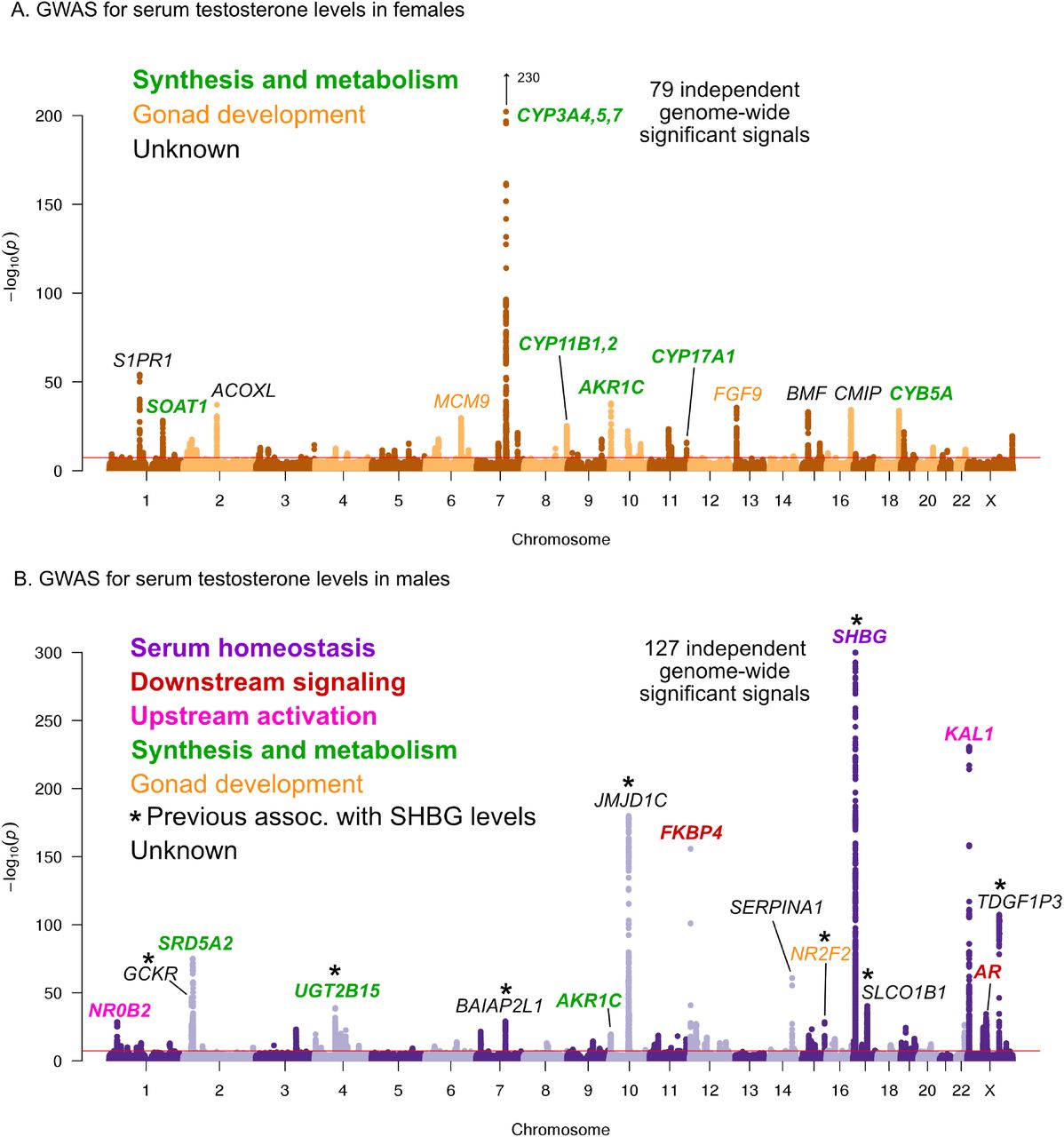
Here, we performed testosterone GWAS in UKBB females (N=142,778) and males (N=146,339) separately. We discovered 79 and 127 independent genome-wide significant signals in females and males, respectively (Figure 5, further details in Supplemental Data 3,4).

Figure 5: Manhattan plots for testosterone.

A. Females. B. Males. Notice the low overlap of lead signals between females and males. FAM9A and FAM9B have been previously proposed as the genes underlying the KAL1 locus [41].

In females, six of the top signals genome-wide are close to genes involved in testosterone biosythesis (Figure 5A); together these results suggest that the steroid biosynthesis pathway is the primary controller of female testosterone levels. Among these, the top hit is at a locus containing three genes involved in hydroxylation of testosterone and estrone, CYP3A4, CYP3A5, and CYP3A7 [49, 50, 51]. Two other lead hits (MCM9 and FGF9) are involved in gonad development [52, 53, 54].

Strikingly, the top hits in males are largely non-overlapping with the top hits in females. Overall, the male hits affect a larger number of distinct processes. Three of the top signals affect the steroid biosynthesis pathway (SRD5A2, UGT2B15, and AKR1C); three are involved in either upstream activation (NR0B2) [55] or downstream signaling (the androgen receptor, AR, and its co-chaperone FKBP4), respectively; and two have been implicated in the development of the GnRH-releasing function of the hypothalamus (KAL1) [56] or the gonads (NR2F2) [57]. However, the largest category, including the top hit overall, is for a group of 8 distinct variants previously shown to affect sex hormone binding globulin (SHBG) levels [58]. SHBG is one of the main binding partners for testosterone–we will discuss the significance of SHBG below.

Steroid biosynthesis

Given our observation of numerous lead hits near steroid hormone biosynthesis genes, we curated the male and female hits in the KEGG pathway (Figure 6). We observed that nearly all major steps of the pathway contained a gene near a genome-wide significant SNP in either females or males: 31 out of 61 genes are within 100kb of a genome-wide significant signal in males, females or both. Indeed, the KEGG steroid hormone pathway shows strong enrichment for signals in both females and males (26-fold enrichment, p = 2.5e-8 in females; 11-fold enrichment, p = 1.2e-4 in males; Figure S6). While this pathway shows clear enrichment in both females and males, the major hits do not overlap. At two loci, AKR1C and PDE2A, male and female hits co-occur at the same locus, but are localized to different SNPs (Figure S7). More broadly, male hits and female hits tend to occur in different parts of the steroid hormone biosynthesis pathway: catalytic steps involved in progestagen and corticosteroid synthesis and metabolism only showed hits in females, while most male hits were concentrated within androgen synthesis, either upstream or downstream of testosterone itself (Figure 6).

Figure 6: Pathway diagram for steroid hormone biosynthesis showing GWAS hits for females and males.

The text color indicates genes within 100kb of a genome-wide significant hit for females (orange), males (blue), or both females and males (black). Grey gene names or numbers indicates genes with no hits. Colored superscripts indicate multiple genes from the same locus (and hence may reflect a single signal). “S*” indicates that an additional, sulfonated metabolite, along with the catalytic step and enzymes leading to it, is not shown. Pathway from KEGG; simplified based on a similar diagram in [59].

Genetics of testosterone regulation in males versus females

One remarkable feature of the testosterone data is the lack of sharing of signals between females and males. This is true for genome-wide significant hits, for which there is no correlation in the effect sizes among lead SNPs (Figure 7A), as well as genome-wide, as the global genetic correlation between females and males is approximately zero (Figure S8).

Figure 7: Sex differences in genetic variation in testosterone

A. When comparing lead SNPs (p < 5e-8 ascertained in either females or males), the effects are nearly non-overlapping between females nd males. Other traits show high correlations for the same analysis (see urate and SHBG in inset). B. Schematic of HPG axis signaling within the hypothalamus and pituitary, with male GWAS hits highlighted. These variants are not significant in females. C. Global genetic correlations, between indicated traits (estimated by LD Score regression). Thickness of line indicates strength of correlation, and significant (p < 0.05) correlations are in bold. Note that LH genetic correlations are not sex-stratified due to small sample size in the UKBB primary care data (N=10,255 individuals). D. Proposed model in which the HPG axis and SHBG-mediated regulation of testosterone feedback loop is primarily active in males. Abbreviations for all panels: SHBG, sex hormone binding globulin; CBAT, calculated bioavailable testosterone; LH, luteinizing hormone.

As we show below, two aspects of testosterone biology can explain these extreme sex differences in genetic architecture. First, the hypothalmic-pituitary-gonadal (HPG) axis plays a more significant role in regulating testosterone production in males than in females. This is due to sex differences in both endocrine signaling within the HPG axis and the tissue sources of testosterone production. Second, SHBG plays an important role in mediating the negative feedback portion of the HPG axis in males but not in females.

To assess the role of HPG signaling, we searched for testosterone GWAS hits involved in the transmission of feedback signals through the hypothalamus and pituitary (Figure 7B, genes reviewed in [60]). We also considered hits from GWAS of calculated bioavailable testosterone (CBAT), which refers to the non-SHBG-bound fraction of total teststerone that is free or albumin-bound, and can be inferred given levels of SHBG, testosterone, and albumin and assuming experimentally determined rate constants for binding [61]. CBAT GWAS thus controls for genetic effects on total testosterone that are mediated by SHBG production.

We found hits for both male testosterone and male CBAT throughout the HPG signaling cascade (Figure 7B). These include genes involved in the direct response of the hypothalamus to testosterone (AR, FKBP4) [62]; modulation of the signal by either autoregulation (TAC3, TACR3) [60] or additional extrinsic endocrine signals (LEPR) [63, 64]; downstream propagation (KISS1) [65] and the development of GnRH-releasing neurons in the hypothalamus (KAL1, CHD7) [66, 67]; and LH-releasing gonadotropes in the pituitary (GREB1) [68]. All of these hits showed more significant effects on CBAT as compared to total testosterone (Figure S10), suggesting that their primary role is in regulating bioavailable testosterone.

Importantly, these HPG signaling hits do not show signals in females. To further investigate the different roles of the HPG axis in males versus females, we performed GWAS of LH levels using UKBB primary care data (N=10,255 individuals). (Recall that LH produced by the pituitary signals to the gonads to promote sex hormone production.) We reasoned that if HPG signaling is important for testosterone production in males but not females, variants affecting LH levels should also affect testosterone levels in males but not females. Consistent with this, we found significant positive genetic correlation between LH and male but not female testosterone (male r_g = 0.27, p = 0.026; female r_g = 0.084, p = 0.49; Figure 7C). These results were similar when considering measured testosterone and LH levels rather than genetic components thereof (Table S1).

Two features of the HPG axis can explain the lack of association in females. First, the adrenal gland, which is not subject to control by HPG signaling, produces ~50% of serum testosterone in females. Indeed, GWAS hits for female testosterone cluster in steroid hormone pathways involving progestagen and corticosteroid synthesis (Figure 6), processes known to occur largely in the adrenal. Female testosterone hits are also specifically enriched for high expression in the adrenal gland relative to male testosterone hits (Figure S11).

Second, for the ovaries, which produce the remaining ~50% of serum testosterone in females, the net effect of increased LH secretion on testosterone production is expected to be diminished. This is because the pituitary also secretes follicle stimulating hormone (FSH), which in females stimulates aromatization of androgens (including testosterone) into estrogens [69]. In males, FSH does not stimulate androgen aromatization but is instead required for sperm production. Consistent with differential roles of FSH, a previously described GWAS hit for menstrual cycle length at FSHB [70] shows suggestive association with testosterone in females but not males (Table S2).

In addition to the role of HPG signaling, the presence of many SHBG-associated variants among the top hits in male testosterone suggests that SHBG also underlies many of the sex-specific genetic effects (Figure 5B). We found high positive genetic correlation between male and female SHBG, as well as between SHBG and total testosterone in males but not females (Figure 7C). Additionally, we found a significant negative genetic correlation between SHBG and CBAT in both females and males, but of a far larger magnitude in females than males (Figure 7C). Together, these observations suggest that while SHBG regulates the bioavailable fraction of testosterone in the expected manner in both females and males, there is subsequent feedback in males only, where decreased CBAT leads to increased total testosterone.

We propose that increased SHBG leads to decreased bioavailable testosterone in both females and males, and in males this relieves the negative feedback from testosterone on the hypothalamus and pituitary gland, ultimately allowing LH production and increased testosterone production (Figure 7D). The lack of SHBG-mediated negative feedback in females is likely due in part to the overall weaker action of the HPG axis, as well as the fact that female testosterone levels are too low to effectively inhibit the HPG axis. This idea is supported experimental manipulations of female testosterone, which result in significant reductions of LH only when increasing testosterone levels to within the range typically found in males [71].

In summary, we find that many of the top signals for female testosterone are in the steroid biosynthesis pathway, and a smaller number relate to gonadal development. In contrast, the lead hits for male testosterone reflect a larger number of processes, including especially SHBG levels and signaling components of the HPG axis, in addition to biosynthesis and gonadal development. These differences in the genetic architecture of male and female testosterone are so extreme that these can be considered unrelated traits.

on by the HPG axis in males but not females.

Polygenic architecture of the three traits

We have shown that the lead signals for all three traits are highly concentrated near core genes and core pathways. Given this observation we wondered whether these traits might be genetically simpler than typical complex diseases–most of which are highly polygenic, and for which the lead pathways contribute relatively little heritability [2, 72].

To address this, we first estimated how much of the SNP heritability is explained by variation at genes in enriched pathways (see Supplemental Data 5-7 for pathways and genes used). We used HESS to estimate the SNP heritability in each of 1701 approximately-independent LD blocks spanning the genome [72, 73]. Plotting the cumulative distribution of SNP heritability across the genome revealed that, across all four traits, most of the genetic variance is distributed nearly uniformly across the genome (Figure 8A).

Figure 8: Despite clear enrichment of core genes and pathways, most heritability for these traits is due to the polygenic background.

(A) Cumulative distribution of SNP heritability for each trait across the genome (estimated by HESS). The locations of the most significant genes are indicated. Insets show the fractions of SNP heritability explained by the most important genes or pathways for each trait. (B) Estimated fractions of SNPs with non-null associations, in bins of LD Score (estimated by ashR). Each point shows the ashR estimate in a bin representing xx% of all SNPs. The inset text indicates the estimated fraction of variants with a non-null marginal effect, i.e. the fraction of variants that are in LD with a causal variant. (C) Simulated fits to the data from (B). X-axis truncated for visualization as higher LD Score bins are noisier. Simulations assume that π₁ of SNPs have causal effects drawn from a normal distribution centered at zero (see Methods). The simulations include a degree of spurious inflation of the test statistic based on the LD Score intercept. Other plausible assumptions, including clumpiness of causal variants, or a fatter-tailed effect distribution would increase the estimated fractions of causal sites above the numbers shown here.

In aggregate, core genes contribute modest fractions of SNP heritability, with the exception of the SLC2A9 locus, which HESS estimates is responsible for 20% of the SNP heritability for urate. Aside from this outlier gene, the major core pathways contribute between 7-11 percent of the SNP heritability, and “secondary” core pathways are between 0.4% – 1.2%.

Numbers of causal variants

We next sought to estimate how many causal variants are likely to contribute to each trait. This is fundamentally a challenging problem, as most causal loci have effect sizes too small to be confidently detected. As a starting point we used ashR, which is an empirical Bayes method that estimates the fraction of non-null test statistics in large-scale experiments [74]. As described previously, we stratified SNPs from across the genome into bins of similar LD Score; we then used ashR to estimate the fraction of non-null associations within each bin [2]. (For this analysis we used the 2.8M SNPs with MAF>5%.) We interpret this procedure as estimating the fraction of all SNPs in a bin that are in LD with a causal variant.

For each trait, the fraction of non-null tests increases from low levels in the lowest LD Score bins to above 50% in the highest LD Score bins. Overall we estimate that around 45-50% of SNPs are linked to a non-zero effect variant for urate, IGF-1 and male testosterone, and 30% for female testosterone (Figure 8B). These estimates were robust to halving the sample size of the input GWAS, and were substantially higher than the mean of ~10% for randomized (phenotype value shuffled) traits (Figure S12).

We next conducted simulations to understand how these observations relate to the numbers of causal variants (Figure 8C). To do this, we simulated phenotypes for the UK Biobank individuals, assuming a range of fractions of causal variants (Methods). Causal variants were chosen uniformly at random from among the 4.4M SNPs with MAF>1%; effect sizes were simulated from a normal distribution with mean zero, and variances set to produce the observed SNP heritabilities (0.3 for urate, IGF-1, and male testosterone, and 0.2 for female testosterone). We also allowed for a degree of over-inflation of the test statistics (i.e., allowing for an inflation factor as in Genomic Control [75])–this was important for fitting the positive ashR estimates at low LD Scores. We then matched the simulations to the observed ashR results to approximate the numbers of causal variants.

Overall, our estimates range from 0.1% of all 4.4M variants with MAF >1% in female testosterone (~4,000 causal sites) to 0.3% of variants for IGF-1 (~12,000 causal sites). These results imply that all four traits are highly polygenic, though considerably less so than height (for which we estimate 2%, or 80,000 causal sites in UK Biobank; Figure S13 and S15).

Furthermore, there are three reasons to suspect that these numbers may be underestimates. First, causal variants are likely to be clumped in the genome instead of being uniformly distributed; simulations with clumping require a larger number of causal variants to match the data (Figure S16). Second, if the distribution of effect sizes has more weight near zero and fatter tails than a normal distribution, this would imply a larger number of causal variants (see analysis assuming a T-distribution, Figure S17). Third, stratified LD Score analysis of the data suggests that some of the apparent evidence for overinflation of the test statistics (Table S3) may in fact be due to a higher proportion of causal variants occurring in lower LD Score bins [76], as the annotation-adjusted intercepts for all traits but height are consistent with 1.

We note that the proportion of causal variants estimated by ashR is substantially lower in low-MAF bins, even in infinitesimal models, presumably due to lower power (Figure S18 and S19). We overcame this by using a parametric fit, which is robust to inflation of test statistics (Figures S20 and S21); the resulting estimates were relatively similar, albeit slightly higher, than when using the simulation-matching method (Figure S15). We note that it is still critical to match samples by heritability and sample size, as in the simulation method (Figure S22), and to use correct covariates in the GWAS (Figure S23).

In summary this analysis indicates that for these molecular traits, around 10-15% of the SNP heritability is due to variants in core pathways (and in the case of urate, SLC2A9 is a major outlier, contributing 20% on its own). However, most of the heritability is due to a much larger number of SNPs spread widely across the genome, conservatively estimated at 4,000-12,000 common variants for the biomarkers and 80,000 for height.

Discussion

In this study, we examined the genetic basis of three molecular traits measured in blood serum: a metabolic byproduct (urate), a signaling protein (IGF-1), and a steroid hormone (testosterone). We showed that unlike most disease traits, these three biomolecules have clear enrichment of genome-wide significant signals in core genes and pathways. At the same time, other aspects of the data are reminiscent of patterns for complex common diseases, including high polygenicity, little indication of allelic dominance or epistasis, and clear enrichment of signals in tissue-specific regulatory elements.

Our main results are as follows.

• Urate: The largest hits for urate are in solute carrier genes in the kidneys that shuttle urate in and out of the blood and urine. Remarkably, eight out of ten annotated urate transporters have genomewide significant signals. A single locus, surrounding SLC2A9, is responsible for 20% of the SNP heritability. The purine biosynthetic pathway, from which urate is produced as a byproduct, is modestly enriched for signals (2.1-fold). Several master regulators for kidney and liver development are among the most significant hits. Aside from SLC2A9, the overall SNP heritability is primarily driven by variants in kidney regulatory regions, both shared across cell types and not.

• IGF-1: IGF-1 is a key component of a signaling cascade that links growth hormone released from the pituitary to stimulation of cell growth in peripheral tissues. We identified 354 independent genome-wide significant signals. The strongest signals lie in genes that interact directly with IGF-1, including IGFBP3, as well as in the IGF1 gene itself. More generally, we see striking enrichment of hits throughout the growth hormone-IGF cascade–this includes especially the upper parts of the cascade, which regulate IGF-1 release, but also in downstream components of the cascade as well, suggesting a feedback mechanism on IGF-1 levels.

• Testosterone: In contrast to urate, testosterone shows clear enrichment of signals within the steroid biosynthesis pathway (26-fold in females, 11-fold in males). Remarkably, the genetic basis of testosterone is completely independent between females and males. In females, the lead hits are mostly involved in synthesis. In males, we see signals throughout the hypothalamic-pituitary-gonadal (HPG) axis which regulates testosterone production in the gonads, as well as in variants that regulate SHBG. Furthermore, in males increased SHBG reduces negative feedback between testosterone levels and the HPG axis, thereby increasing total serum testosterone.

• Polygenic background. For each of these traits, the core genes and pathways contribute only a modest fraction of the total SNP heritability. Aside from SLC2A9 for urate, the most important core pathways contribute up to about 10% of the total SNP heritability. We estimated the numbers of causal variants under a model where causal variants have a normal effect-size distribution. We estimate that there are around 4,000-12,000 common variants with non-zero effects on these traits. Using the same method we estimated about 80,000 causal sites for height. These estimates are likely conservative as several of our assumptions may lead us to underestimate the true values.

The architecture of complex traits and the omnigenic model

One of our primary motivations in this study was to use these three traits as models to extend our understanding of the architecture of complex traits.

Many of the advances of 20th century genetics came from reductionist approaches that focused on understanding the functions of major-effect mutations; this principle has been extended in the GWAS era into interpreting the impact of lead signals. And yet, at the same time, most heritability is driven by the polygenic background of small effects at genes that are not directly involved in the trait. The overwhelming importance of the polygenic background is a striking discovery of modern GWAS, and demands explanation as it does not fit neatly into the standard conceptual models of the relationship between genotype and phenotype.

Our group has recently proposed a simplified conceptual model to understand this [2, 3]. We proposed that for any given trait there is a set of core genes that are directly involved in the biology of the phenotype. We proposed that (1) core genes are only responsible for a small fraction of phenotypic variance, and that (2) most phenotypic variance is controlled by a sum of weak transregulatory perturbations from other expressed genes (“peripheral” genes) that affect expression of the core genes. In support of this model, we noted that even for a trait as relatively simple as gene expression, most of the phenotypic variance comes from large numbers of small trans effects. We proposed that in the “omnigenic” limit, one may expect that essentially every gene expressed in relevant cell types has the potential to exert a nonzero effect on a given phenotype–though of course most of these effects will be exceedingly small, and not every gene has cis-regulatory variation and thus in practice many do not contribute.

However, for most disease traits it is currently difficult to evaluate this model. We generally do not know core genes or pathways with any accuracy, and it is difficult to determine why most hits are linked to disease. Thus, the three molecular traits considered here provide valuable examples to better understand complex trait architecture. For all three traits we find huge enrichment of top signals at core genes within the primary pathways that regulate these traits. At the same time, these core pathways only explain modest fractions of the heritability, and most heritability is due to a polygenic background of ~ 10⁴ variants. Consequently, these traits provide compelling illustrations of our model.

Moreover, we can expect that disease endpoints–which are usually products of many highly polygenic biological traits such those studied here–will even be far more polygenic than the molecular traits studied here. Most diseases and other traits depend on the combinations of inputs from many other phenotypes including the phenotypes considered here [77].

Examples for some of the factors that affect diabetes and heart attack are shown in Figure 9. Mendelian randomization shows contributions from all three of our biomarkers to diabetes or cardiovascular disease risk [7, 48]. As a more extreme example, behavioral traits such as educational attainment are notoriously polygenic [78], and these are affected by complicated networks of other aspects of health and behavior [79]. The point here is that when multiple risk factors–each of which is polygenic–contribute to any given disease, the disease endpoint absorbs the polygenic basis for all of the risk factors together.

Figure 9: Disease endpoints are often affected by contributions from multiple other inputs, each of which are themselves polygenic

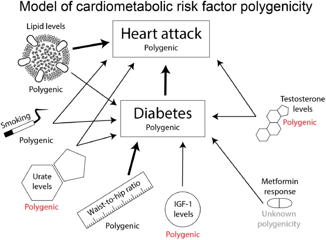
Here we show a few of the risk factors that contribute to diabetes and heart attack. The genetic basis of the disease endpoint can be modeled as a weighted sum of the genetic effects for all the input traits, which will further increase its polygenicity.

In summary, we have shown that for these three molecular traits, the lead hits illuminate core genes and pathways to a degree that is highly unusual in GWAS. By doing so they illustrate which processes may be most important for trait regulation. For example, for urate, kidney transport is more important than biosynthesis, while for testosterone, biosynthesis is important in both sexes but especially in females. However, in other respects the GWAS data here are reminiscent of more-complex traits: in particular most trait variance comes from a huge number of small effects at peripheral loci. Lastly, these vignettes help to illustrate why many diseases are extraordinarily polygenic, as they are usually impacted by multiple biological processes that, like those considered here, are themselves highly polygenic.

Data availability

GWAS summary statistics generated for this study will be deposited on the GWAS Catalog. GWAS summary statistics and Supplemental Data tables are available at http://web.stanford.edu/group/pritchardlab/dataArchive.html.

Methods

Population definition

We defined our GWAS population as a subset of the UK Biobank [6]. We use ~337,000 unrelated White British individuals as our cohort, filtering based on sample QC characteristics as previously described [7]:

1. Used to compute principal components (used_in_pca_calculation column)

2. Not marked as outliers for heterozygosity and missing rates (het_missing_outliers column)

3. Do not show putative sex chromosome aneuploidy (putative_sex_chromosome_aneuploidy column)

4. Have at most 10 putative third-degree relatives (excess_relatives column).

5. Finally, we used the in_white_British_ancestry_subset column in the sample QC file to define the subset of individuals in the White British cohort.

Trait definition

We perform trait normalization and quality control similarly to previous work [7]. Trait measurements are first log-transformed, then adjusted for genotype principal components, age indicator variables, sex, 5-year age (‘approximate age’) by sex interactions, self-identified ethnicity, self-identified ethnicity by sex interactions, fasting time, estimated sample dilution factor, assessment center, genotyping batch, 20-tile of time of sampling, month of assessment, and day of assay.

Then, individuals were subset to the GWAS population (defined above), separated by sex for testosterone measurements. The final sample sizes were 318,526 for urate, 317,114 for IGF-1, 142,778 for female testosterone, and 146,339 for male testosterone.

GWAS

We performed GWAS in plink2 alpha using the following command (data loading arguments removed for brevity):

GWAS were then filtered to observed allele frequency greater than 0.001 and INFO score greater than 0.3 for further analyses.

GWAS for paired difference epistasis

A GWAS was performed in two subsets of individuals – those with two C alleles at rs16890979 (N = 295209) and those with two T alleles at rs16890979 (N = 30184). The following command was used:

With covariates including adjusting for age, age squared, genotyping array, and 20 principal components. The residual urate levels, already adjusted for age, sex, global principal components, and technical covariates (Methods) were used as input.

After GWAS completed, SNPs valid in both CC and TT individuals were compared for betas using a paired difference Z test. The test statistic was then converted to a P-value using a standard normal distribution.

LH trait definition

LH levels were extracted from UK Biobank primary care data using code XM0lv. Separately, LH levels extracted using code XE25I were also included for phenotypic correlation analyses. The median level across observations and log number of observations were recorded for covariate correction below. Individuals with median observations more than 10 times the interquartile range away from the median of medians were discarded. Once these individuals were removed, individuals with observations more than four standard deviations from the resulting mean were also discarded.

For the primary LH code XM0lv, the distribution of raw, cleaned, and covariate-adjusted phenotype values were respectively:

For the secondary LH code XE25I, the distribution of raw, cleaned, and covariate-adjusted phenotype values were respectively:

For GWAS, the cleaned phenotypes were log-transformed and adjustments were used as covariates.

LH GWAS

Age, sex, genotyping array, 10 PCs, log number of observations in primary care, and which primary care code produced a given observation were used as covariates.

We performed GWAS in plink2 alpha using the following command (data loading arguments removed for brevity):

We also performed GWAS of LH code XE25I in a sex stratified fashion using the following command:

On genotyped SNPs and imputed variants with a minor allele frequency greater than 1% in the White British as a whole.

GWAS were then filtered to MAF > 1% and INFO > 0.7. These higher threshold were chosen to reflect the much smaller sample size in the GWAS.

GWAS hit processing

To evaluate GWAS hits, we took the list of SNPs in the GWAS and ran the following command using plink1.9:

We then took the resulting independent GWAS hits and examined them for overlap with genes. In addition, for defining the set of SNPs to use for enrichment analyses, we greedily merged SNPs located within 0.1 cM of each other and took the SNP with the minimum p-value across all merged lead SNPs. In this way, we avoided potential overlapping variants that were driven by the same, extremely large, gene effects.

Gene proximity

We annotated all genes in any Biocarta, GO, KEGG, or Reactome MSigDB pathway as our full list of putative genes (in order to avoid pseudogenes and genes of unknown function), and included the genes within each corresponding pathway as our target set. This resulted in 17847 genes. We extended genes by 100kb (truncating at the chromosome ends) and used the corresponding regions, overlapped with SNP positions, to define SNPs within range of a given gene. Gene positions were defined based on Ensembl 87 gene annotations on the GRCh37 genome build.

Pathway enrichment of GWAS hits

GWAS hit pathway enrichment was evaluated using Fisher’s exact test. For each pathway for a given trait (Supplemental Data 5-7), genes were divided into those within the pathway and those outside; and separately into genes within 100kb of a GWAS hit and not. A 2×2 Fisher’s exact test was used to estimate the total enrichment for GWAS hits around genes of interest.

For male and female testosterone, we noticed a number of GWAS loci with multiple paralogous enzymes within the synthesis pathway (e.g. AKR1C, UGT2B, CYP3A). To avoid double counting GWAS hits when testing enrichment at such loci, we instead considered the number of GWAS hits (within 100 kb of any pathway gene as above) normalized to the total genomic distance covered by all genes (+/− 100kb) in the pathway. A Poisson test was used to compare the rate parameter for this GWAS hit/Mb statistic between genes in a given pathway and all genes not in the pathway.

Partitioned heritability

Partitioned heritability estimates were generated using LD Score regression [21]. The BaselineLD version 2.2 was used as a covariate, and the 10 tissue type LD Score annotations were used as previously described [21] in a multiple regression setup with all cell type annotations and the baseline annotations.

Pathway heritability estimation

We evaluated heritability in pathways using two distinct strategies. Initially, we used partitioned LD Score regression [21] but found that the estimates were somewhat noisy, likely because most pathways contain few genes. As such, we used alternative fixed-effect models for which there is increased power.

Next, we calculated the heritability in a set of 1701 approximately independent genomic blocks spanning the genome [73] using HESS [72]. Next, we overlapped blocks with genes in each pathway. The heritability estimates for all blocks containing at least one SNP within 100kb of a pathway gene were summed to estimate the heritability in a given pathway. Pathway definitions were assembled based on a combination of KEGG pathways, Gene Ontology categories, and manual curation based on relevant reviews.

Causal SNP simulations

All imputed variants with MAF > 1% in the White British (4.1M) were used as a starting set of putative causal SNPs. Individual causal variants were chosen at random, with a fraction P of them marked as causal. Each causal variant was assigned an effect size:

For our simulations, we used P ∈ {0.0001, 0.001, 0.003, 0.01, 0.03}.

Next, GCTA was used to simulate phenotypes based on the marked causal variants, using the following command:

Producing predicted phenotypes with heritability h² = 0.3. GWAS were run within both the full set of 337,000 unrelated White British individuals and a randomly downsampled 50%, to approximate the sex-specific GWAS used for Testosterone, across the set of putative causal SNPs. GWAS for the traits, as well as a random permuting across individuals of urate and IGF-1 to act as negative controls, were repeated on this subset of variants as well. In this way, we have a directly comparable set of simulated traits to use, along with the corresponding true traits and negative controls, to ascertain causal sites in the genome.

For the infinitesimal simulations, instead plink was used to generate polygenic scores on the basis of the random assignment of effect sizes to SNPs, and these were then normalized with N(0, σ²) environmental noise such that h² was the given target heritability.

Causal SNP count fitting procedure using ashr

LD Scores for the 489 unrelated European-ancestry individuals in 1000 Genomes Phase III [80] were merged with the GWAS results along with LD Scores derived from unrelated European ancestry participants with whole genome sequencing in TwinsUK. TwinsUK LD Scores are used for all analyses. Then variants were filtered by minor allele frequency to either greater than 1%, greater than 5%, or between 1% and 5%. Remaining variants were divided into 1000 equal sized bins, along with 5000 and 200 bin sensitivity tests. Within each bin, the ashR estimates of causal variants, as well as the mean χ² statistics, were calculated using the following line of R:

Thus, the within-bin χ² and proportion of null associations π₀ were each ascertained. Next, these fits were plotted as a function of mean.ld to estimate the slope with respect to LD Score, and true traits were compared to simulated traits, described below.

We use two fixed simulated heritabilities, h² = 0.3 and h² = 0.2, to approximately capture the set of heritabilites observed among our biomarker traits. Traits with true SNP heritability among variants with MAF > 1% different than their closest simulation might have causal site count over-estimated (for ) or under-estimated (for ). In addition, most traits in reality have more than zero SNPs with MAF < 1% contributing to the heritability. Thus, we take these estimates as approximate and conservative.

Effect of population structure on causal SNP estimation

We expect that population structure might lead to test statistic inflation for causal variant and genetic correlation estimates [81]. To evaluate this, we performed GWAS for height using no principal components, and evaluated the causal variant count (Figure S23).

This suggests that the test statistic inflation is an important parameter in the estimation of causal variants, as is intuitive. As such, we generated estimated SNP counts for five different inflation values (0.9, 1, 1.05, 1.1, and 1.2) and plotted all of them, under the assumption that the best fitting intercept would have the most calibrated estimates. Plots are replicated across these intercepts in the sensitivity analyses shown, as in Figure S20.

Evaluating the calibration of causal SNP proportion estimation

To evaluate calibration of causal SNP estimates, in addition to using simulated traits as the controls, we also generated a randomized control by shuffling the SHBG phenotype values across individuals (Figure S14). We performed this analysis using urate and IGF-1 to similar effect (data not shown).

This suggests that the causal variant counts are well calibrated for the randomized traits, even though they lack structure with respect to covariates.

Effect of sample size on causal SNP estimation

It is important to note that these estimates are still likely power limited even in a study as large as UK Biobank. We make this note on the basis of observed π₀ for MAF > 5% variants being uniformly higher than 1% < MAF < 5% variants in both simulations and observed data for high causal variant counts (Figure S19).

As such, we anticipate that future studies with larger samples will yield increased, but asymptotic, estimates of causal SNP percentages among common variants, and treat our estimates as conservative bounds.

Particularly for height (Figure S13), while the uncalibrated estimates with the full sample are substantially higher than the half sample, the calibrated estimates are nearly identical. This suggests that trait polygenicity might be an important factor in determining the power of this method at different sample sizes, as height is known to be highly polygenic [72].

Effect of binned variant count on causal SNP estimation

It is possible that the ashR algorithm itself, and not the GWAS, are the power limited step of the analysis. To evaluate this, we ran ashR on 200, 1000, and 5000 equally sized bins along the LD Score axis. We found that increasing bin counts both decrease the standard errors and the intercepts (Figure S24) and recommend as many bins as is practical.

Effect of minor allele frequency on causal SNP estimation

Because we only simulated causal effects among SNPs with MAF > 1%, we were concerned that variant effect bins might be biased by the minor allele frequency cutoff. We previously ran with higher MAF cutoffs (25% and 40%) as calibrations on an earlier version of the model, and observed uniformly larger causal SNP percentages. We saw relative robustness to lower thresholds, but overall the fraction of causal variants was lower in the lower MAF bins (Figure S18).

Effect of concentrated SNPs on causal SNP estimation

For each variant, the megabase bin it is contained within was used as a proxy for SNPs in local LD. A within-megabase causal SNP percentage parameter: was chosen such that ρ was the overall expected percentage of causal sites in the genome across a concentration parameter α. For our simulations, we used ρ ∈ {0.0001, 0.0003, 0.001, 0.003, 0.01, 0.03, 0.05} and α ∈ {10, 3, 0.3} to represent different degrees of “clumpiness” along the genome.

Genetic correlation between sex-stratified testosterone-related traits

LD Score regression [?] was used to generate genetic correlation estimates. The following command was used: where eur_*_ld_chr were downloaded from https://data.broadinstitute.org/alkesgroup/LDSCORE/.

Residual height comparison with IGF-1

Height (adjusted for age and sex) and residualized log IGF-1 levels for unrelated White British individuals were plotted against each other, and visualized using geom_smooth.

Pathway diagrams

Diagrams were drawn using Adobe Illustrator and a Wacom graphics tablet.

PheWAS analysis

PheWAS were performed using the Oxford Brain Imaging Genetics (BIG) Server [82].

Non-additivity tests

Residualized trait values were used as the outcome in all models. An ANOVA was performed between a model measuring the effect of genotype dosages versus a model with both genotype dosage effects and indicators for each rounded genotype. In this way, a large number of possible non-additive models are approximated with a single model. Analyses were performed in R 3.4 using lm.

Epistasis tests

Residualized trait values were used as the outcome in all models. An ANOVA was performed between a model measuring the effect of indicators for each rounded genotype (4 degrees of freedom) versus the interaction between the two sets of indicators (8 degrees of freedom). In this way, a large number of possible non-additive models are approximated with a test. Alternative models with dominant-only effect interactions with fewer degrees of freedom were also tested with similar results. Analyses were performed in R 3.4 using lm.

LD Score regression for partitioning heritability

We used partitioned LD Score regression [21] to estimate the enrichment of individual tissues. We used the ldsc package and the updated BaselineLD v2.2 annotations with the following command:

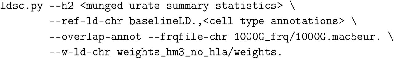
Where <cell type annotations> were alternative either the default annotations for each of the ten cell type groups [21] or modified versions which were filtered of any regulatory regions overlapping with the kidney cell type, using the following command:

In this way, the cell type exclusive, non-kidney regulatory elements are used.

Acknowledgments

We thank members of the Pritchard, Page, Przeworski, Sella, and Bassik labs, as well as Evan Boyle, Eric Fauman, Jake Freimer, Yang Li, Xuanyao Liu, Iain Mathieson, Molly Przeworski, Guy Sella, Jeff Spence, and Rebecca Harris for helpful discussions; and the UK Biobank and its participants for making this project possible, which we accessed through UK Biobank application number 24983. This work was supported by NIH grants HG008140 and HG009431, a Stanford Graduate Fellowship (to N.S.-A.), and a National Defense Science and Engineering Grant (to N.S.-A.).

Footnotes

• * Joint First Authors

• http://web.stanford.edu/group/pritchardlab/dataArchive.html