

Abstract
Various pre-trained deep-learning models for the segmentation of biomedical images have been made available to users with little to no knowledge in machine learning. However, testing these tools individually is tedious and success is uncertain.
Here, we present OpSeF, a Python framework for deep-learning based semantic segmentation that was developed to promote the collaboration of biomedical user with experienced image-analysts. The performance of pre-trained models can be improved by using pre-processing to make the new input data more closely resemble the data the selected models were trained on. OpSeF assists analysts with the semi-automated exploration of different pre-processing parameters. OpSeF integrates in a single framework: scikit-image, a collection of Python algorithms for image processing, and three mechanistically distinct convolutional neural network (CNN) based segmentation methods, the U-Net implementation used in Cellprofiler 3.0, StarDist, and Cellpose. The optimization of parameters used for preprocessing and selection of a suitable model for segmentation form one functional unit. Even if sufficiently good results are not achievable with this approach, OpSeF results can inform the analysts in the selection of the most promising CNN-architecture in which the biomedical user might invest the effort of manually labeling training data.
We provide two generic non-microscopy image collections to illustrate common segmentation challenges. Further datasets exemplify the segmentation of a mono-layer of fluorescent cells, fluorescent tissue, cells in which various compartments have been stained with a single dye, as well as histological sections stained with one or two dyes. We provide Jupyter notebooks to support analysts in user training and as a template for the systematic search for the best combination of preprocessing and CNN-based segmentation. Results can be analyzed and visualized using matplotlib, pandas, scikit-image, and scikit-learn. They can be refined by object-selection based on their region properties, a biomedical-user-provided or an auto-generated mask. Additionally, results might be exported to AnnotatorJ for editing or classification in ImageJ. After refinement, the analyst can re-import results and further analyze them in OpSeF.
We encourage biomedical users to provide further image collections, analysts Jupyter notebooks, and pre-trained models. Thereby, OpSeF might soon become, both a “model store”, in which appropriate model might be identified with reasonable effort and a valuable resource for teaching biomedical user CNN-based segmentation.
Introduction
Phenomics, the assessment of the set of physical and biochemical properties that completely characterize an organism, has long been recognized as one of the greatest challenges in modern biology (Houle et al., 2010). Microscopy is a crucial technology to study phenotypic characteristics. Advances in high-throughput microscopy (Lang et al., 2006; Neumann et al., 2010; Chessel and Carazo Salas, 2019), slide scanner technology (Webster and Dunstan, 2014; Wang et al., 2019), light-sheet microscopy (Swoger et al., 2014; Ueda et al., 2020), semi-automated (Bykov et al., 2019; Schorb et al., 2019) and volume electron microscopy (Titze and Genoud, 2016; Vidavsky et al., 2016), as well as correlative light- and electron microscopy (Hoffman et al., 2020) have revolutionized the imaging of organisms, tissues, organoids, cells, and subcellular structures. Due to the massive amount of data produced by these approaches, the traditional biomedical image analysis tool of “visual inspection” is no longer feasible, and classical, non-machine-learning based image analysis is often not robust enough to extract phenotypic characteristics reliably in a non-supervised manner.
Thus, the advances mentioned above were enabled by breakthroughs in the application of machine learning methods to biological images. Traditional machine learning techniques, based on random-forest classifiers and support vector machines, were made accessible to biologists with little to no knowledge in machine learning, using stand-alone tools such as ilastik (Haubold et al., 2016; Berg et al., 2019; Kreshuk and Zhang, 2019) or QuPath (Bankhead et al., 2017). Alternatively, they were integrated into several image analysis platforms such as Cellprofiler (Lamprecht et al., 2007), Cellprofiler Analyst (Jones et al., 2009), Icy (de Chaumont et al., 2012), ImageJ (Schneider et al., 2012; Arganda-Carreras et al., 2017) or KNIME (Sieb et al., 2007).
More recently, deep learning methods, initially developed for computer vision challenges, such as face recognition or autonomous cars, have been applied to biological image analysis. The U-Net was the first deep convolutional neural network specifically designed for semantic segmentation of biomedical images (Ronneberger et al., 2015). Segmentation challenges like the 2018 Data Science Bowl (DSB) further promoted the adaptation of computer vision algorithms like Mask R-CNN (He et al., 2017) to biological analysis challenges (Caicedo et al., 2019). The DSB included various classes of nuclei. Schmidt and colleagues use the same dataset to demonstrate that star-convex polygons are better suited to represent crowded cells (Schmidt et al., 2018) than axis-aligned bounding boxes used in Mask R-CNN (Hollandi et al., 2019). Training of deep learning models typically involves the tedious painting of the ground truth. Approaches that address this limitation include optimizing the painting by starting with reasonable good predictions (Hollandi and Horváth, 2020), adaptation of the preprocessing such that existing model can be used (Whitehead, 2020), and the use of generalist algorithm trained on highly variable images (Stringer et al., 2020). Following the latter approach, Stringer and colleagues trained a neural network to predict vector flows generated by the reversible transformation of a highly diverse image collection. Their model works well on specialist and generalized data (Stringer et al., 2020).
Various pre-trained deep-learning models for the segmentation of biomedical images have been made available to users with little to no knowledge in machine learning (Hollandi et al., 2019; Weigert et al., 2019; Stringer et al., 2020). However, testing these tools individually is tedious and success is uncertain.
Pre-trained models might fail, because the network was trained on data that does not resemble the new images well. Alternatively, the underlying network architecture might not be suited for the presented task. Biomedical users with no background in computer science are often unable to distinguish these two possibilities and might erroneously conclude that their problem is in principle not suited for deep-learning-based segmentation. Thus, they might hesitate to create annotations to retrain the most appropriate architecture. Here, we present OpSeF IV, a Python framework for deep-learning-based semantic segmentation of cells or nuclei. OpSeF has primarily been developed for staff image analysts with solid knowledge in image analysis, thorough understating of the principles of machine learning, and basic skills in Python. It integrates scikit-image, a collection of Python algorithms for image processing (van der Walt et al., 2014), the U-Net implementation used in Cellprofiler 3.0 (McQuin et al., 2018), StarDist (Schmidt et al., 2018), and Cellpose (Stringer et al., 2020). Jupyter notebooks serve as a minimal graphical user interface. Most computation is performed head-less. Segmentation results can be easily imported and refined in ImageJ using AnnotatorJ (Hollandi and Horváth, 2020).
Material and Methods
Data description
Cobblestones
Images of cobblestones were taken with a Samsung Galaxy S6 Active Smartphone.
Leaves
Noise was added to the demo data from “YAPiC - Yet Another Pixel Classifier” available at https://github.com/yapic/yapic/tree/master/docs/example_data using the Add Noise function in ImageJ.
Small fluorescent nuclei
Images of Hek293 human embryonic kidney stained with a nuclear dye from the image set BBBC038v1(Caicedo et al., 2019) available from the Broad Bioimage Benchmark Collection (BBBC). Metadata is not available for this image set to confirm staining conditions. Images were rescaled from 360×360 pixels to 512×512 pixels.
3D colon tissue
We used low-signal to noise variant of the image set BBBC027 (Svoboda et al., 2011) from the BBBC.
Epithelial cells
Images of cervical cells from the image set BBBC038v1 (Caicedo et al., 2019) available from the BBBC. Cells were stained with a dye that labels membranes weakly and nuclei strongly. The staining pattern is reminiscent of images of methylene blue-stained cells. However, metadata is not available for this image set to confirm staining conditions.
Skeletal muscle
A methylene-blue-stained skeletal muscle section was recorded on a Nikon Eclipse Ni-E microscope equipped with a Märzhäuser SlideExpress2 system for automated handling of slides. The pixel size is 0.37*0.37 μm. Thirteen patches 2048×2048 pixels large patches were manually extracted from the original 44712×55444 pixels large image. Color images were converted to grey-scale.
Kidney
A HE stained kidney paraffin sections were recorded on a Nikon Eclipse Ni-E microscope equipped with a Märzhäuser SlideExpress2 system for automated handling of slides. The pixel size is 180 × 180 nm. The original, stitched, 34816 × 51200 pixels large image was split into two large patches (18432 × 6144 and 22528 × 5120 pixel). Next, the Eosin staining was extracted using the Color Deconvolution ImageJ plugin. This plugin implements the method described by Ruifrok and Johnston(Ruifrok and Johnston, 2001).
Algorithm
Various deep-learning based models have been made available to users, either in the context of collections or as a stand-alone tool. However, testing these individually, each time optimizing the preprocessing for best results, is tedious, in particular for staff image analysts who are confronted with different segmentation tasks on a daily or weekly basis. OpSeF has been designed to accelerate the optimization of CNN-based segmentation and to integrate results seamlessly in complex image analysis pipelines.
OpSeF’s analysis pipeline consists of four principal sets of functions to import and reshape the data, to preprocess it, to segment objects, and to analyze and classify results (Figure 1A). Currently, OpSeF can process individual tiff-files and the proprietary Leica “.lif” container file format. During import and reshape, the following options are available for tiff-input: tile in 2D and 3D, scale, and make sub-stacks (Figure 1B). For lif-files, only the make sub-stacks option is supported (Figure 1B). Preprocessing is mainly based on scikit-image (van der Walt et al., 2014). It consists of a linear pipeline (Figure 1C) in which images are filtered in 2D, the background is removed, and stacks are projected. Next, the following optional preprocessing operations might be performed: histogram adjustment (Zuiderveld, 1994), edge enhancement, and inversion of images. Available segmentation options include the pre-trained U-Net used in Cellprofiler 3.0 (McQuin et al., 2018), the StarDist 2D model (Schmidt et al., 2018) and Cellpose (Stringer et al., 2020). Preprocessing and selection of the ideal model for segmentation are one functional unit. Figure 1D illustrates this concept with a processing pipeline, in which three different models are applied to four different preprocessing pipelines each. The resulting images are classified into results that are mostly correct, suffer from under- or over-segmentation or largely fail to detect objects. In the given example, the combination of preprocessing pipeline three and model two gives overall the best result. We recommend an iterative optimization which starts with a large number of models, and relatively few, but conceptually distinct preprocessing pipelines. Next, the number of models to be explored might be reduced, while fine-tuning the most promising preprocessing pipelines. Results can be analyzed and visualized using matplotlib, pandas, scikit-image, and scikit-learn (Figure 1E and Figure 2A-C). They might be refined by object selection based on their region properties (Figure 2B), a user-provided (Figure 2D) or an autogenerated mask. Additionally, results might be exported to AnnotatorJ (Hollandi and Horváth, 2020) for editing or classification in ImageJ. AnnotatorJ is an ImageJ plugin that helps hand-labeling data with deep learning-supported semi-automatic annotation and further convenient functions to easily create and edit object contours. It has been extended with a classification mode and import/export fitting the data structure used in OpSeF. After refinement, results can be re-imported and further analyzed in OpSeF. Analysis options include scatter plots of region properties (Figure 2B), T-distributed Stochastic Neighbor Embedding (t-SNE) analysis (Figure 2F) and principal component analysis (PCA) (Figure 2G).

Analysis pipeline (A) Overview: The analysis pipeline consists of four groups of functions used to import and reshape the data, to preprocess it, to segment objects, and to analyze and classify results. (B) Import and Reshape: The following options are available for tiff-input: tile in 2D and 3D, scale, and make sub-stacks. For lif-files, only the make sub-stacks option is supported. (C) Preprocessing is mainly based on scikit-image. It consists of a linear pipeline: Images are filtered in 2D, background is removed, and stacks are projected. Next, the following preprocessing operations may be performed: histogram equalization, edge enhancement, and inversion of images. Variables used to define processing parameters are displayed in italics. (D) Optimization procedure. Left panel: Illustration of a processing pipeline, in which three different models are applied to data generated by four different preprocessing pipelines each. Right panel: Resulting images are classified into results that are correct; suffer from under- or over-segmentation or fail to detect objects. (E) Illustration of post-processing pipeline. Segmented objects might be filtered by their region properties or a mask, results might be exported to AnnotatorJ and re-imported for further analysis. Blue arrows define the default processing pipeline, grey arrows feature available options. Dark blue boxes are core components, light blue boxes are optional processing steps.

Example of how post-processing can be used to refine results (A) StarDist segmentation of the multi-labeled cells dataset detected nuclei reliably but caused many false positive detections. These resemble the typical shape of cells but are larger than true nuclei. Orange arrows point at nuclei that were missed, the white arrow at two nuclei that were not split, the blue arrows at false positive detections that could not be removed by filtering. (B) Scatter plot of segmentation results shown in A. Left panel: Mean intensity plotted against object area. Right panel: Circularity plotted against object area. Blue Box illustrating the parameter used to filter results. (C) Filtered Results. Orange arrows point at nuclei that were missed, the white arrow at two nuclei that were not split, the blue arrows at false positive detections that could not be removed by filtering. (D,E) Example for the use of a user provided mask to classify segmented objects. The segmentation results (false colored nuclei) are superimposed onto the original image subjected to [median 3×3] preprocessing. All nuclei located in the green area assigned to Class 1, all others to Class 2. Red box indicates region shown enlarged in (E). From left to right in E: original image, nuclei assigned to class 1, nuclei assigned to class 2. (F) T-distributed Stochastic Neighbor Embedding (t-SNE) analysis of nuclei assigned to class 1 (purple) or class 2 (yellow). (G) Principal component analysis (PCA) of nuclei assigned to class 1 (purple) or class 2 (yellow).
Data and Source code availability
Test data for the jupyter notebooks is available at: https://owncloud.gwdg.de/index.php/s/nSUqVXkkfUDPG5b
Test data for AnnotatorJ is available at: https://owncloud.gwdg.de/index.php/s/dUMM6JRXsuhTncS
The source code is available at: https://github.com/trasse/OpSeF-IV
Results
We evaluated the potential of OpSeF IV to: elucidate efficiently whether a given segmentation task is solvable with state of the art deep convolutional neural networks (CNNs), optimizing preprocessing, assessing whether the chosen model performs well without retraining and testing, and how well it generalizes in heterogeneous datasets.
Preprocessing can be used to make the input image more closely resemble the data on which the models for the CNNs bundled with OpSeF were trained on. Additionally, preprocessing steps can used to normalize data and reduce heterogeneity. Generally, there will be not be a single, universal best preprocessing pipeline. Instead, well-performing combinations of preprocessing pipelines and matching CNN-models will be found. Even the metric for what constitutes a good result will vary from project to project, depending on the biological question posed. For cell tracking, very reproducible cell identification will be of utmost importance; for other applications, the accuracy of the outline might be more crucial. To harness the full power of CNN-based segmentation models and to build trust in their more widespread use, it is essential to understand under which conditions they are prone to fail.
We use various demo datasets to challenge the CNN-based segmentation pipelines. Jupyter notebooks document how OpSeF was used to obtain reliable results. These notebooks are provided as a starting point for the iterative optimization of user projects and as a tool for interactive user training.
The first two datasets - cobblestones and leaves - are generic, non-microscopic image collections, designed to illustrate common analysis challenges. Further datasets exemplify the segmentation of a monolayer of fluorescent cells, fluorescent tissues, cells in which various compartments have been stained with the same dye, as well as histological sections stained with one or two dyes. The latter dataset exemplifies additionally, how OpSeF can be used to process large 2D images.
Objects in the cobblestone dataset are approximately square-shaped. In contrast, nuclei and cells are typically of round or ellipsoid shaped. Heterogeneous intensities within objects and in the border region, as well as a five-fold variation of object size, further challenge segmentation pipelines. In the first round of optimization, minor smoothing [median filter with 3×3 kernel (median 3×3)] and background subtraction were applied. Next, the effect of additional histogram equalization, edge enhancement, and image inversion was tested. The resulting four preprocessed images were segmented with all models [Cellpose nuclei, Cellpose Cyto, StarDist, and U-Net]. The Cellpose scale-factor range [0.2,0.4,0.6] was explored. Among the 32 resulting segmentation pipelines, the combination of image inversion and the Cellpose Cyto 0.4 model produced, without further optimization, the best results in both training images (Figure 3A,B). The segmentation generalized well to the entire dataset. Only in one image, three objects were missed, and one object was over-segmented. Borders around these stones are very hard to distinguish for a human observer, and even further training might not resolve the presented segmentation tasks (Figure 3E,F). Cellpose has been trained on a large variety of images and had been reported to perform well on objects of similar shape (compare Figure 4, Images 21,22,27 in (Stringer et al., 2020)).
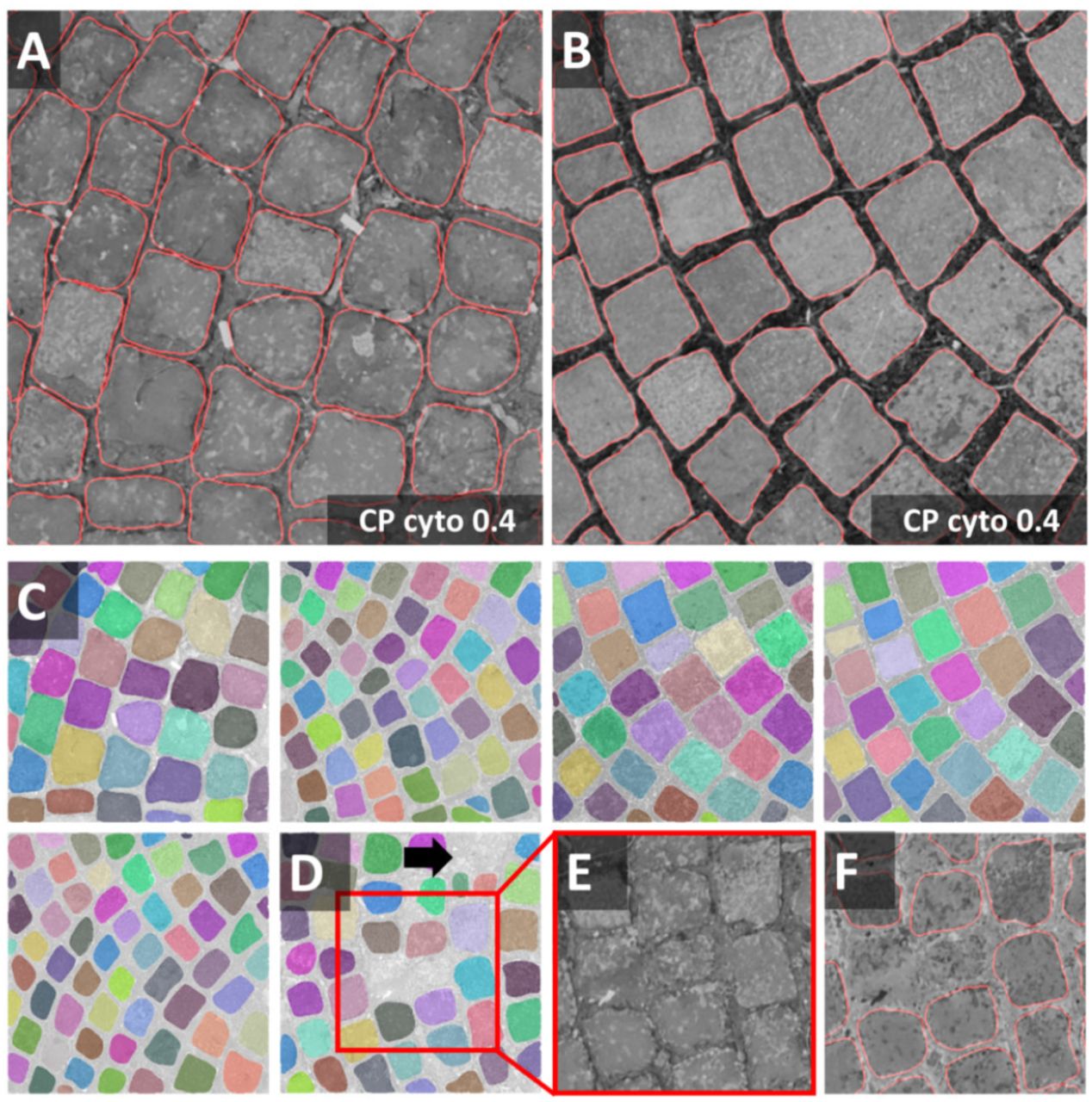
Cobblestones notebook (A,B) Segmentations (red line) of the Cellpose Cyto model are superimposed onto the original image subjected to [median 3×3] preprocessing. The inverted image (not shown) was used as input to the segmentation. Outlines are well defined, no objects were missed, none over-segmented. These settings fit accurately to the entire dataset (train and test) shown in (C,D). Only in one image, three objects were missed and one was over-segmented. Borders around these stones are hard to discern. Individual objects are false color-coded in C,D. The red squares in D highlight one of the two problematic regions shown as a close-up in (E) and (F).
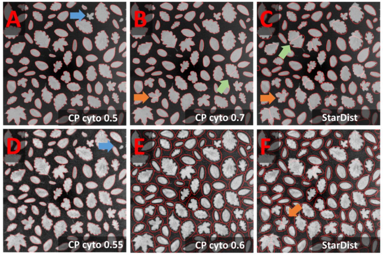
Leaves notebook (A-C) Segmentation results (red line) of the Cellpose Cyto and 0.7 model are superimposed onto the original image subjected to [median 3×3] preprocessing. The inverted image (not shown) was used as input to the segmentation. Outlines are well defined, few objects were missed (A: blue arrow), some over-segmented (B,C: green and orange arrow). Green arrow points at an oak leave with prominent leaf veins, orange arrow at maple leaves with less prominent leave veins. (D-F) Results of further optimization. Further smoothing (E) reduced the rate of false negatives (blue arrow) and over-segmentation in the Cellpose Cyto model. However, object outlines were less precise (E).
Segmentation of the leaves dataset seems trivial and could easily be solved by any threshold-based approach. Nevertheless, it challenges CNN-based segmentation due to non-typical shapes, dark lines, objects vary 20-fold in area, and heterogeneous background. Preprocessing was performed as described for the cobblestone dataset. The most promising result was obtained with the Cellpose Cyto 0.5 model in combination with [median 3×3 & image inversion] preprocessing (Figure 4A,B) and the StarDist model with [median 3×3 & histogram equalization] preprocessing (Figure 4C). Outlines were well defined, few objects were missed (blue arrow in Figure 4A), few over-segmented (green and orange arrow in Figure 4B,C). The Cellpose Cyto 0.7 model gave similar results.
Maple leaves (orange arrows in Figure 4B,C) were most frequently over-segmented. Their shape resembles a cluster of touching cells. Thus, the observed over-segmentation might be caused by the attempt of the CNN to reconcile their shapes with structures it has been trained on. Oak leaves were the second most frequently over-segmented leave type. These leaves contain dark leave veins that might be interpreted as cell borders. However, erroneous segmentation mostly does not follow these veins (green arrow in Figure 4B). Next, the effect of stronger smoothing [mean 7×7] was explored. For the Cellpose nuclei model (Figure 4E), it reduced the rate of false-negative detections (Figure 4D blue arrow) and over-segmentation (Figure 4F orange arrow) at the expense of loss in precision of object outlines. Parameter combinations tested in Figure 4D,E generalize well in the entire dataset.
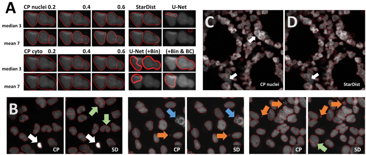
Next, we used OpSeF to segment nuclei in a monolayer of cells. Most nuclei are well separated. We focused our analysis on the few nuclei that touch. Both the Cellpose nuclei model and the Cellpose Cyto model performed well across a broad range of scale-factors. Interestingly, strong smoothing made the Cellpose nuclei but not the Cellpose Cyto model more prone to over-segmentation (Figure 5A). The StarDist model performed well; the U-Net failed. The latter was surprising, given the task is seemingly simple. The pixel intensities have a small dynamic range, and nuclei are dim and rather large. To elucidate whether any of these issues led to this poor performance, we binned the input 2×2 (U-Net+BIN panel in Figure 5A) and adjusted brightness and contrast. Adjusting brightness and contrast alone had no beneficial effect (data not shown). The U-Net performed much better on the binned input. We next batch-processed the entire dataset. StarDist was more prone to over-segmentation (green arrow in Figure 5B), but detected smaller objects more faithfully (orange arrow in Figure 5B) and was more likely to include atypical objects, e.g. nuclei during cell division that display a strong texture (blue arrow in Figure 5B). Substantial variation in brightness was well tolerated by both models (white arrow in Figure 5B). Both models complement each other well.

Fluorescent nuclei notebook (A) Segmentation of the sparse nuclei data set. Example of two touching cells. The segmentation result (red line) superimposed onto the original image subjected to [median 3×3] preprocessing. Columns define the model used for segmentation, the rows the filter used for preprocessing. Cellpose nuclei model and the Cellpose Cyto model performed well across a large range of scale-factors. The U-Net failed initially. Improved results after binning are shown in the lower right panel. (B) Comparison of Cellpose nuclei (CP) and StarDist (SD) segmentation results (red line). StarDist is more prone to over-segmentation (green arrow), but detects smaller objects more reliably (orange arrow) and tends to include objects with strong texture (blue arrow). Strong variation in brightness was tolerated well by both models (white arrow). (C,D) Segmentation of 3D colon tissue from the Broad BioImage Benchmark Collection with Cellpose nuclei (CP) or StarDist (SD). Both models gave reasonable results. Only a few dense clusters could not be segmented (white arrow).
Next, we tested a more complex dataset: 3D colon tissue from the Broad Bioimage Benchmark Collection. This synthetic dataset is ideally suited to assess segmenting clustered nuclei in tissues. We chose the low signal-to-noise variant, which allowed us to test strategies to suppress noise. Sum, maximum and median projection of three Z-planes was tested in combination with the preprocessing variants previously described for the monolayer of cells dataset. Twelve different preprocessing pipelines were combined with all models [Cellpose nuclei, Cellpose Cyto, StarDist, and U-Net]. The Cellpose scale-factor range [0.15, 0.25, 0.4, 0.6] was explored. Many segmentation decisions in the 3D colon tissue dataset are even for human experts hard to perform. Within this limitation, [median projection & histogram equalization] preprocessing produced reasonable results without any further optimization in combination with either Cellpose nuclei 0.4 or the StarDist model (Figure 5C,D). Only a few cell clusters were not segmented (Figure 5C,D white arrow). Both models performed equally well on the entire data set.
We next tried to segment a single layer of irregular shaped epithelial cells, in which the nucleus and cell membranes had been stained with the same dye. In the first run, minor [median 3×3] or strong [mean 7×7] smoothing was applied. Next, the effect of additional histogram equalization, edge enhancement, and image inversion was tested. The resulting eight preprocessed images were segmented with all models [Cellpose nuclei, Cellpose Cyto, StarDist, and U-Net]. The Cellpose scale-factor range [0.6, 0.8, 1.0, 1.4, 1.8] was explored. The size of nuclei varied more than five-fold. We thus focused our analysis on a cluster of particular large nuclei and a cluster of small nuclei. The Cellpose nuclei 1.4 and StarDist model detected both small and large nuclei similar well (Figure 6A). StarDist segmentation results included many cell-shaped false-positive detections. As they were in general much larger than true nuclei, they can be filtered out during post-processing. While the U-Net did not perform well on the same input [median 3×3] (Figure 6A), it returned better results (Figure 6A) upon [mean 7×7 & histogram equalization] preprocessing. As weak smoothing was beneficial for the Cellpose and StarDist pipelines and stronger smoothing for the U-Net pipelines, we explored the effect of intermediate smoothing [median 5×5] for Cellpose and StarDist and even stronger smoothing [mean 9×9] for the U-Net pipelines. A slight improvement was observed. Thus, we used [median 5×5] preprocessing in combination with Cellpose nuclei 1.5 or StarDist model to process the entire dataset. Cellpose frequently failed to detect bright, round nuclei (Figure 6B, arrows) and StartDist had many false detections. Thus, retraining or post-processing is required.

Multi-labeled cells notebook (A) Images of large epithelial cells from the 2018 Data Science Bowl collection were used to test the segmentation of a single layer of cells. These cells vary in size. The Cellpose nuclei 1.4 model and [median 3×3] preprocessing gave a reasonable segmentation for big and small nuclei. StarDist segmentation based on the same input detected nuclei more reliably. However, many false-positive detections were present. Interestingly, the shape of false detections resembles the typical shape of cells well. The U-Net did not perform well with the same preprocessing, but with [mean 7×7 & histogram equalization] preprocessing. (B) [Median 5×5] preprocessing in combination with the Cellpose 1.5 nuclei or the StarDist model was applied to the entire data set. The Cellpose model missed reproducibly round, very bright nuclei (blue arrow) and StarDist predicted many false-positive cells (right panel).
In the DSB, most algorithms performed better on images classified as small or large fluorescent, compared to images classified as “purple tissue” or “pink and purple” tissue. We used methylene-blue stained skeletal muscle sections as a sample dataset for tissue stained with a single dye and Hematoxylin and eosin (HE) stained kidney paraffin sections as an example for multi-dye stained tissue. Analysis of tissue sections might be compromised by heterogenous image quality cause e.g. by artifacts created at the junctions of tiles. Thus, all workflows used the fused image as input to the analysis pipeline.
While most nuclei in the skeletal muscle dataset are well separated, some form dense cluster, other nuclei are out of focus (Figure 7A). The size of nuclei varies ten-fold; their shape ranges from elongated to round. The same preprocessing and model as described for the epithelial cells dataset were used; the Cellpose scale-factor range [0.2, 0.4, 0.6] was explored. [Median 3×3 & invert image] preprocessing combined with the Cellpose nuclei 0.6 model produced without further optimization satisfactory results (Figure 7B). Outlines were well defined, some objects were missed, few over-segmented. Neither StarDist nor the U-Net performed similar well. We could not overcome this limitation by adaptation of preprocessing or binning. Processing of the entire dataset identified in-adequate segmentation of dense cluster (Figure 7C, white arrow) and occasional over-segmentation of large, elongated nuclei (Figure 7C, orange arrow) as the main limitation. Nuclei that are out-of-focus were frequently missed (Figure 7C, blue arrow). Limiting the analysis to in-focus nuclei is feasible.

Skeletal muscle notebook (A) An methylene-blue-stained skeletal muscle section was used to test the segmentation of tissue that has been stained with one dye. (B) Segmentation was tested on 2048×2048 pixels large image patches. The star shown in A and B is located at the same position within the image displayed at different zoom factors. The segmentation result (red line) of the Cellpose nuclei 0.6 model is superimposed onto the original image subjected to [median 3×3] preprocessing. (C,D) Close-up on regions that were difficult to segment. Segmentation of dense cluster (white arrow) often failed, and occasional over-segmentation of large, elongated nuclei (orange arrow) was observed. Nuclei that are out-of-focus (blue arrow) were frequently missed (blue arrow).
Cell density is very heterogeneous in the kidney dataset. The Eosin signal from a HE stained kidney paraffin section (Figure 8A,B) was obtained by color deconvolution. Nuclei are densely packed within glomeruli and rather sparse in the proximal and distal tubules. Two stitched images were split using OpSeF’s “to tiles” function. Initial optimization was performed on a batch of 16 image tiles, the entire dataset contains 864 tiles. The same preprocessing and model as described for the skeletal muscle dataset were used, the Cellpose scale-factor range [0.6, 0.8, 1.0, 1.4, 1.8] was explored. [Median 3×3 & histogram equalization] preprocessing in combination with the Cellpose nuclei 0.6 model produced good results (Figure 8C). [Mean 7×7 & histogram equalization] preprocessing in combination with StarDist performed similarly well (Figure 8C). The latter pipeline resulted in more false-positive detections (Figure 8C, purple arrows). The U-Net performed less well, and more nuclei were missed (Figure 8C, blue arrow). All models failed for dense cell clusters (Figure 8C,D, white arrow).

Kidney notebook (A,B) Part of a HE stained kidney paraffin section used to test segmentation of tissue stained with two dyes. White box in A highlights the region shown enlarged in B. Star in A,B,D marks the same glomerulus. (C)Eosin signal was extracted by color deconvolution. The segmentation result (blue line) is superimposed onto the original image subjected to [median 3×3] preprocessing. Cellpose nuclei 0.6 model with scale-factor 0.6 in combination with [median 3×3 & histogram equalization] preprocessing and the StarDist model with [mean 7×7 & histogram equalization] performed similar well (C,D). StarDist resulted in more false-positive detections (purple arrows). The U-Net performed less well, more nuclei were missed (blue arrow). All models failed in very dense areas (white arrow).
Discussion
Intended use and future developments
Examining the relationship between biochemical changes and morphological alterations in diseased tissues is crucial to understand and treat complex diseases. Traditionally, microscopic images are inspected visually. This approach limits the possibilities for the characterization of phenotypes to more obvious changes that occur later in disease progression. The manual investigation of subtle alterations at the single-cell level, which often require quantitative assays, is hampered by the data volume. A whole slide tissue image might contain over one million cells. Despite the improvement in machine learning technology, completely unsupervised analysis pipelines have not been widely accepted. Thus, one of the major challenges for the coming years will be the development of efficient strategies to keep the human-expert in the loop. Many biomedical users still perceive deep-learning models as black boxes. The mathematical foundation how CNNs decide is improving and OpSeF facilitates understanding the pit-falls of CNN-based segmentation on a more descriptive level. Collectively, increased awareness of limitations and better interpretability of results will be pivotal to increase the acceptance of machine learning methods. It will improve the quality control of results and allow for efficient integration of expert knowledge in analysis pipelines (Holzinger et al., 2019a; Holzinger et al., 2019b).
As illustrated in the provided Jupyter notebooks, the U-Net often performed worst. Why is that the case? As previously reported the learning capacity of a single U-Net is limited (Caicedo et al., 2019). Thus, the provision of a set of U-Nets trained on diverse data might be a promising approach to address this limitation, in particular in combination with dedicated pre- and post-procession pipelines. OpSeF allows for the straightforward integration of a large number of pre-trained CNNs. We hope that OpSeF will be widely accepted as a framework through which novel models might be made available to other image analysts in an efficient way.
OpSeF allows for semi-automated exploration of a large number of possible combinations of preprocessing pipelines and segmentation models. Even if sufficiently good results are not achievable with preprocessing and pre-trained models, OPSEF results may be used as a guide for which CNN architecture, the effort of labeling is reinvested. The generation of training data is greatly facilitated by a seamless integration in ImageJ using the AnnotatorJ plugin. We hope that many OpSeF users will contribute their training data to open repositories and will make new models available for integration in OpSeF. Thus, OpSeF might soon become, both a “model store”, in which appropriate model might be identified with reasonable effort. Community provided Jupyter notebooks might be used to teach students in courses how to optimize CNN based analysis pipelines. This will educate them and make them less dependent on turn-key solutions that often trade performance for simplicity and offer little to no insight into reasons why the CNN-based segmentation works or fails. The better users understand the model they use, the more they will trust them, the better they will be able to quality control them.
Integrating various segmentation strategies and quality control of results
Multiple strategies for instance segmentation have been pursued. The U-Net belongs to the “pixel to object” class of methods: each pixel is first assigned to a semantic class (e.g., cell or background), then pixels are grouped into objects (Ronneberger et al., 2015). Mask R-CNNs belong to the “object to pixel” class of methods (He et al., 2017): initial prediction of bounding boxes for each object is followed by a semantic segmentation. Following an intermediate approach, Schmidt and colleagues predict first star-convex polygons that approximate the shape of cells, and use then non-maximum suppression to prune redundant predictions (Schmidt et al., 2018; Weigert et al., 2019). Stringer and colleagues use stimulated diffusion originating from the center of a cell to convert segmentation masks into flow fields. The neural network is then trained to predict flow fields, which can be converted back into segmentation masks (Stringer et al., 2020). Each of these methods has specific strengths and weaknesses. The use of flow fields as auxiliary representation proved to be a great advantage for predicting cell shapes that are not roundish. At the same time, Cellpose is the most computationally demanding model used. In our hands, Cellpose tended to result in more obviously erroneously missed objects, in particular, if objects displayed a distinct appearance compared to their neighbors (blue arrows in Figure 5B, Figure 6B, and Figure 7D). StarDist is much less computationally demanding, and star-convex polygons are well suited to approximate elliptical cell shapes. The pre-trained StarDist model implemented in OpSeF might be less precise in predicting other convex shapes it has not been trained on. However, this limitation might be overcome by retraining. Many shapes e.g. maple leaves (Figure 4C), are concave, and StarDist can - due to “limitation by design” - not be expected to segment these objects precisely. Segmentation errors by the StarDist model were generally plausible. It tended to predict cell-like shapes, even if they are not present (Figure 6B). Although the tendency of StarDist to fail gracefully might be advantageous in most instances, this feature requires particular careful quality control to detect and fix errors. The “pixel-to-object” class of methods are less suited for segmentation of dense cell clusters. The misclassification of just a few pixel might lead to the fusion of neighboring cells.
OpSeF integrates three mechanistically distinct methods for CNN-based segmentation in a single framework. This allows comparing these methods easily. Nonetheless, we decided against integrating determining F1 score, false positive and false negative rates and accuracy. Firstly, because in a large class of applications no ground-truth is available. Secondly, we want to encourage the user to visually inspect segmentation results. Inspecting 100 different segmentation results opened in ImageJ as stack takes only a few minutes and gives valuable insight into when and how segmentations fail. This knowledge is easily missed when just looking at the output scores of commonly used metrics. Learning more about the circumstances in which certain types of CNN-based segmentation fail helps to decide when human experts are most essential for quality control of results. Moreover, it is pivotal for the design of post-processing pipelines that select among multiple segmentation hypothesis - on an object by object basis - the one, which gives the most consistent results for reconstructing complex cells-shapes in large 3D volumes or for cell-tracking.
Optimizing results and computational cost
Image analysis pipelines are generally a compromise between ease-of-use and performance as well as between computational cost and accuracy. Until now, the rather simple U-Net is - despite its limited learning capacity - of the most frequently used model in the major image analysis tools. In contrast, the winning model of the 2018 Data Science Bowl by the [ods.ai] topcoders team used sophisticated data post-processing to combine the output of 32 different neural networks (Caicedo et al., 2019). High computational cost currently limits the widespread use of this or similar approaches. OpSeF is an ideal platform to find the computationally most efficient solution to a segmentation task. The [ods.ai] topcoders algorithm was designed to segment five different classes of nuclei: small and large fluorescent, grayscale, purple and pink and purple tissue (Caicedo et al., 2019). Stringer and colleagues used an even broader collection of images that included cells of unusual appearance and natural images of regular cell-like shapes such as shells, garlic, pearls and stones (Stringer et al., 2020).
The availability of such versatile models is precious, in particular, for users, who are unable to train custom models or lack resources to search for the most efficient pretrained model. For most biological applications, however, no one-fits-all solution is required. Instead, potentially appropriate models might be pre-selected, optimized and tested and using OpSeF. Ideally, an image analyst and a biomedical researcher will jointly fine-tune the analysis pipeline and quality control results. This way, resulting analysis workflows will have the best chances of being both robust and accurate, and an ideal balance between manual effort, computational cost, and accuracy might be reached.
Comparison of the model available within OpSeF IV revealed that the same task of segmenting 100 images using StarDist took 1.5-fold, Cellpose with fixed scale-factor 3.5-fold, and Cellpose with flexible scale-factor 5-fold longer compared to segmentation with the U-Net.
The systematic search of the optimal parameter and ideal performance might be dispensable if only a few images are to be processed that can be easily manually curated, but highly valuable if massive datasets produced by slide-scanner, light-sheet microscopes of volume EM techniques are to be processed.
Deployment strategies
We decided against providing OpSeF as an interactive cloud solution. A local solution uses existing resources best, avoids limitations generated by the down- and upload of large datasets, and addresses concerns regarding the security of clinical datasets.
Author Contributions
T.M.R. designed and developed the OpSeF. R.H. and P.H. designed and developed the AnnotatorJ integration. Data was analyzed by T.M.R. Manuscript was written by T.M.R. with contributions from all authors.
Acknowledgments
We would like to thank Volker Hilsenstein from Monash Micro Imaging for testing of the software and for critical comments on the manuscript; the IT service group of the Max Planck Institute for Heart and Lung Research for technical support. We thank anyone who made their data available, in particular: the Broad Bioimage Benchmark Collection for image set BBBC027 (Svoboda et al., 2011) and BBBC038v1 (Caicedo et al., 2019) and Christoph Möhl. We thank developers of all software that was integrated into OpSeF or used in this paper, in particular: Cellpose, Cellprofiler, ImageJ, matplotlib, numpy, pandas, scikit-learn, scikit-image and StarDist and Tensorflow.
Research in the Scientific Service Group Microscopy was funded by the Max Planck Society. PH and RH acknowledge the LENDULET-BIOMAG Grant (2018-342) and from the European Regional Development Funds (GINOP-2.3.2-15-2016-00006, GINOP-2.3.2-15-2016-00026, GINOP-2.3.2-15-2016-00037).


