

Abstract
A pervasive issue in stable isotope tracing and metabolic flux analysis is the presence of naturally occurring isotopes such as 13C. For mass isotopomer distributions (MIDs) measured by mass spectrometry, it is common practice to correct for natural isotopes within metabolites of interest using a particular linear transform based on binomial distributions. However, the origin and mathematical derivation of this transform is rather obscure, and it may be difficult for nonexperts to understand precisely how to interpret the resulting corrected MIDs. Moreover, corrected MIDs are often used to fit metabolic network models and infer metabolic fluxes, which implicitly assumes that corrected MIDs will yield the same flux solution as the actual observed MIDs. Yet, there seems to be no published proof of this important property. Here, we provide a detailed derivation of the MID-correcting linear transform, reflecting its historical development, and describe some interesting properties. We also provide a proof that for metabolic flux analysis on noise-free MID data at steady state, observed and corrected MIDs indeed yield the same flux solution. On the other hand, for noisy MID data, the flux solution will generally differ between the two representations.
1 Introduction
When analyzing data from stable isotope tracing experiments, the presence of naturally occurring isotopes can be problematic. For example, carbon-13 (13C) accounts for about 1% of all carbon in the biosphere [Berglund and Wieser, 2011], and when measuring metabolic products we must somehow correct for this natural 13C to determine the amount of 13C derived from a tracer [Buescher et al., 2015]. Obviously, there is no physical difference between naturally occurring and tracerderived 13C, so this correction can only be made statistically. To make this notion precise, we will need some definitions. For mass spectrometry data, an n-carbon compound can be divided into n + 1 mass isotopomers (also called isotopologues), where mass isotopomer i represents the set of molecules of the compound that contain exactly i 13C atoms (i = 0, 1, …, n), regardless of their position in the molecule. We will consider only 13C in this paper, but other isotopes such as 15N or 2H can be handled similarly. The associated mass isotopomer distribution (MID) is an (n + 1)-vector x = (x0 x1 … xn)T where xi is the fraction of molecules having i 13C atoms. (Throughout, we will index MID vectors and related matrices starting from zero for convenience.) Because natural 13C atoms occur randomly and independently with a probability p ≈ 0.01, the “natural” mass isotopomer distribution (MID) of an n-carbon compound is a vector βn whose elements follow the binomial distribution

In isotope tracing experiments, natural-derived and tracer-derived 13C inevitably mix to form the observed MIDs. An MID correction method is then a function that maps any observed MID x to a hypothetical MID y that would have been observed if natural 13C did not exist. We refer to y as a corrected MID. In particular, MID correction must map the natural MID βn to the unit vector en,0 = (1 0 … 0)T. Over the years, several methods and software packages have been developed for MID correction [Millard et al., 2012, Jungreuthmayer et al., 2015, Su et al., 2017, Millard et al., 2019], providing various features such as support for multiple isotopes and compound fragmentation. They are all based on a particular class of linear transforms Tn, n = 1, 2, … that relate an n-carbon MID x to the corrected MID y as x = Tny, where Tn is the (n + 1) × (n + 1) matrix

MID correction then simply amounts to solve this system for y = (Tn)−1x (the matrix Tn is always invertible). However, it is difficult to find literature explaining how this particular transform is derived and demonstrating why the MID y is indeed a corrected MID, as defined above. The transform Tn was developed in a series of technical studies going back as far the 1960’s [Brauman, 1966], but these may be inaccessible to non-experts, and so the origin and underlying logic of the transform Tn remains somewhat obscure. An excellent survey of the historical development of MID correction was given by Midani et al. [2017], but did not include a mathematical derivation of the transform Tn. In section 2 of this paper, we provide such a derivation, reflecting the historical development. We then discuss some interesting properties of Tn in section 3.
Another important question arises when the corrected MIDs y are used for metabolic flux analysis (MFA). Performing MFA on corrected MIDs is attractive since we need not keep track of natural isotopes, simplifying the analysis [Buescher et al., 2015]. But, cellular metabolism obviously acts on the “uncorrected” MIDs x that physically occur, and therefore MFA on these uncorrected MIDs (where “unlabeled” molecules have binomial MIDs βn) must be regarded as the ground truth. Therefore, to ensure that MFA on the corrected MIDs y is valid, we must first establish that this always yields the same results as MFA on the actual MIDs x. To our knowledge there is no published proof of this proposition. We provide such a proof for the case of noise-free data at isotopic steady-state in section 4, and conclude by discussing some remaining open questions.
2 Derivation of the MID correction
To understand the origin of the MID correcting transform Tn, we here provide a derivation reflecting its historical development [Midani et al., 2017]. We will first review mixture models of MIDs, which constitute a related but somewhat different type of “correction” that yields the fractional abundance of one or more tracers in a metabolite pool, thereby accounting for natural 13C. We then describe a general model for the MID of labeled compounds that occur in mixture models, and finally show how these models can be generalized to obtain the transform Tn.
2.1 Linear mixtures of tracers
We first consider the simple case where an n-carbon tracer with known MID x1 is mixed with an endogenous source of the same compound, which has natural MID x0 = β6 (Figure 1). At steady state, the observed (measured) MID x is then a linear mixture
 where a0, a1 are the mixture fractions (satisfying a0 + a1 = 1). This situation typically arises in isotope tracing in vivo, where x0 is known as the tracee [Cobelli et al., 1992]. Provided that we know the tracer MID x1 and can measure the MID x, the above yields n + 1 equations and two unknowns, and we can solve for the mixture coefficients a = (a0, a1) using a least-squares method [Brauman, 1966]. For the example data given in Figure 1, this gives a = (0.85, 0.15), indicating that the tracer constitutes 15% of the observed mixture, after “correction” for natural 13C. As expected, a1 < x1 = 0.191, since natural 13C also contributes to x1. It is straightforward to extend this model to multiple tracers with MIDs x1, x2, …, xK,


A tracer-tracee example. (A) An endogenous 6-carbon compound with natural MID x0 = β6 is mixed with a 1-13C tracer x1 in proportions a0, a1, forming a mixture with MID x. Black circles indicate 13C atoms, gray circles atoms drawn from the natural isotope distribution. (B) Example (hypothetical) MID data from the system in A.
Provided that K ≤ n, we can still solve for the mixture coefficients ak.
An important generalization is to apply the above mixture model also in cases where some of the mixture components are metabolic products. For example, Rosenblatt et al. [1992] described a case where a doubly labeled leucine tracer is metabolized to a singly labeled one, and both are mixed with endogenous leucine (Figure 2). To solve this model, we must of course know the MID x1 of the biologically synthesized 13C1-leucine, as well as the tracer MID x2. Since x1 cannot be observed experimentally, Rosenblatt et al. [1992] suggested to instead use a theoretical distribution, which we will describe next.

Mixture model adapted from Rosenblatt et al. [1992], with some simplifications. Here a 13C2 leucine tracer with MID x2 is metabolized to a 13C1-leucine compound (x1), and both are mixed with endogenous leucine (x0), with mixture coefficients ak.
2.2 The MID of labeled compounds
In this section, we describe the MID of an n-carbon compound that has incorporated k atoms from a pure 13C source and n − k atoms from a natural distribution, 0 ≤ k ≤ n. Denote this MID τn,k. For the special case k = 0 we simply have τn,0 = βn, while for k = n we have the pure 13Cn MID τn,n = en,n. For 0 < k < n, we assume that the n-carbon compound is formed by a condensation between a pure 13Ck compound with MID τk,k and a naturally distributed compound with MID τn−k,0 (see Figure 3A for an example). The resulting MID τn,k of the condensation product is then given by the convolution
 where x ⊗ y is defined component-wise as

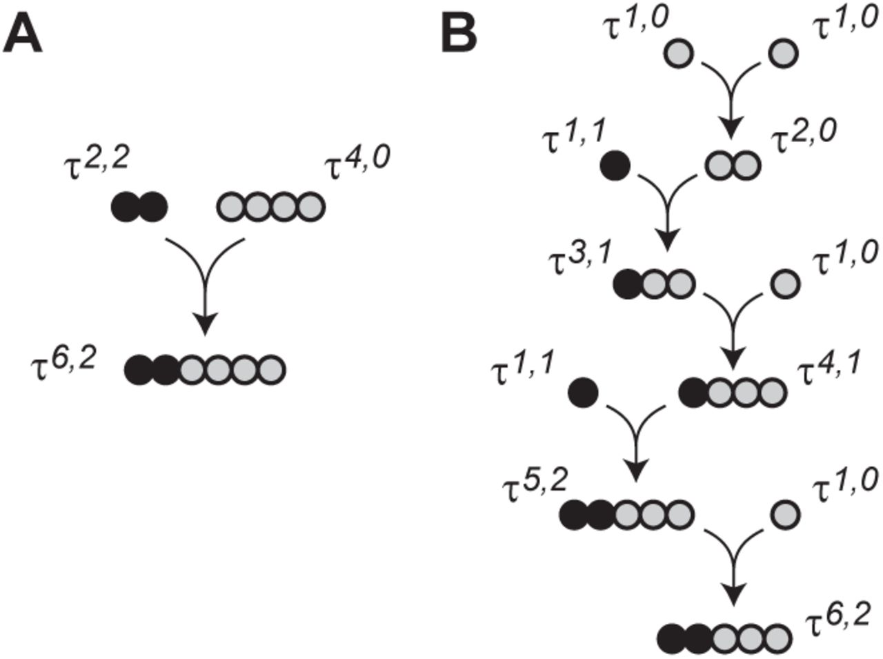
(A) Condensation between a pure 13C2 compound with MID τ2,2 and a C4 compound with natural distribution τ4,0 = β4, yielding the MID τ6,2. (B) Example of step-wise condensations of pure 13C atoms with natural 13C atoms, resulting in the same MID τ6,2.
It is straightforward to show that this convolution yields the MID
 where 0k denotes the k-dimensional zero vector. That is, convoluting a natural MID with the unit vector ek,k will “shift” the MID by k steps. For example, the labeled compounds in Figure 2 would have MIDs

This model based on condensations reflects how larger molecules are synthesized by anabolic pathways, which is indeed how most tracers are produced: for example, the MID τ6,2 might be produced by a condensation τ6,2 = τ2,2 ⊗ τ4,0 (Figure 3A). Moreover, any sequence of condensations (in any order) that incorporate a total of k 13C atoms from a pure 13C source and n − k atoms from a natural carbon source will generate same MID τn,k. This is because a condensation between any two τ distributions always yields another τ distribution,
 since the ⊗ operator is commutative and associative, and it holds that βm ⊗ βn = βm+n for any m, n. Applying this property repeatedly, we see that an MID τn,k can be formed from 1-carbon building block as
 where the condensations can occur in any order. For example, Figure 3B shows one possible sequence of condensations giving rise to τ6,2 = τ2,2 ⊗ τ4,0.
With the class of distributions τn,k, we can now model all MIDs in the example of Figure 2 as x0 = τ6,0, x1 = τ6,1 and x2 = τ6,2, and this generalizes to any mixture of compounds produced by condensations. However, the resulting mixture MID x in Figure 2 is not itself a τ distribution.
2.3 From mixture models to MID correction
We now derive the general case of the MID correcting transform Tn from the distributions τn,k. Fernandez et al. [1996] described the case of an arbitrary n-carbon molecule formed as a mixture of n + 1 compounds with distributions τn,0, τn,1, …, τn,n, defined as above. We can write the resulting mixture model in matrix form as
 where a is again the vector of mixture coefficients, and Tn is the (n + 1) × (n + 1) matrix
 whose columns are the MID vectors of the mixed compounds. Comparing with (2), we see that this is exactly the MID correction matrix (1), if the vector of mixture coefficients a can be interpreted as the corrected MID y. To understand why this interpretation is valid, consider the following thought experiment (Figure 4).
For any metabolite with any MID x, we can partition the population of molecules into n + 1 subpopulations, where subpopulation k consists of those molecules that have incorporated k13C atoms from a pure 13C source and n−k atoms from a natural source, k = 0, 1, …, n (Figure 4A). Then, the MID of subpopulation k is precisely τn,k, and ak is the the fraction of molecules belonging to this sub-population, and we again have the mixture MID x = Tna. Now, imagine that we could replace all natural-derived 13C in these molecules with 12C (Figure 4B). Then the MID of subpopulation k would simply be the unit vector en,k, and therefore the mixture MID becomes identical to the mixture coefficients,  . Therefore, the vector a can be interpreted as the MID y that we would have obtained if natural 13C did not exist, that is, the corrected MID.

A thought experiment. (A) A pool of molecules partitioned into sets based on the number of 13C atoms derived from a pure 13C source (black). Gray indicates atoms drawn from the natural isotope distribution. (B) The same partition, with natural-distributed atoms replaced by 12C atoms (white). For details, see text.
In summary, we have demonstrated that for any n-carbon compound formed by combining combining pure 13C carbon with natural-distributed carbon, the observed MID x and the corrected MID y are related as x = Tny. This model is valid for any product of a metabolic network whose substrates are either pure 13C (en,n) or natural (βn).
3 Properties of the transform Tn
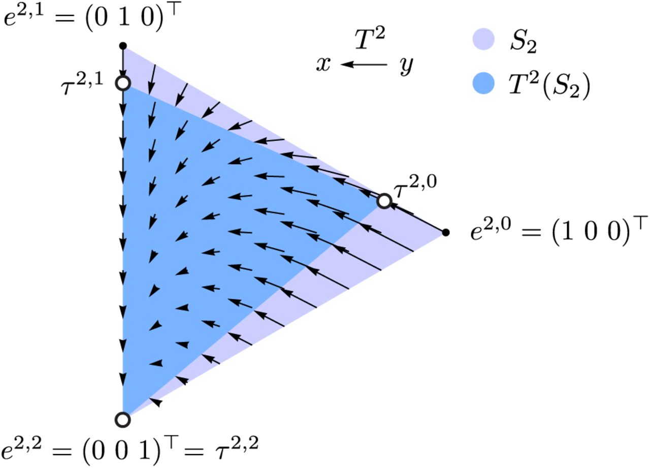
In this section, we discuss some interesting properties of the transform Tn. To gain a bit of intuition, Figure 5 visualizes the effects of Tn for the case n = 2 at various points in the 2-simplex S2. (The n-simplex Sn is the set  , that is, the set of all possible n-carbon MIDs.) As with any linear operator, Tn maps the k’th unit vector en,k to the MID given by the k’th column of Tn, Tnen,k = τn,k, k = 0, …, n. A special case is k = n for which Tnen,n = τn,n = en,n.

The effect of the transform T2 (for a 2-carbon compound) on MID vectors in the 2-simplex S2, drawn projected from R3 into the plane. Arrows indicate the effect of applying T2 at various points y ∈ S2. Dark blue region is the image T2(S2) of the 2-simplex, whose corners are the MIDs τ2,k, k = 0, 1, 2. Here the heavy isotope probability p was set to 0.1 for clarity.
This is the only eigenvector of Tn that lies within the simplex Sn, reflecting the fact that a pure 13Cn compound cannot have incorporated natural 13C. All other vectors y ∈ Sn are “pushed” towards en,n by Tn (Figure 5). Conversely, (Tn)−1 maps each MID τn,k to the unit vector en,k, and in particular maps the natural MID τn,0 = βn to the unit vector en,0. It is in this sense that (Tn)−1 “removes” natural 13C. However, it should be noted that there is nothing about the corrected MID y = (Tn)−1x that distinguishes it as inherently free of natural 13C: we could in principle observe the same MID y from another measurement. This is evident from the fact that (Tn)−1 is not a projection, as (Tn)−1(Tn)−1x ≠ (Tn)−1x.
It is important to note that, while Tn is invertible, is it not surjective. It is clear that if y ∈ Sn, then x = Tny is also in Sn, since Tny is a convex combination of the columns of Tn, all of which are in Sn. But not all vectors x ∈ Sn can be written as x = Tny; that is, the image of Tn(Sn) does not cover all of Sn (Figure 5). For example, no unit vector en,k for k < n is in Tn(Sn). The part of Sn that lies outside Tn(Sn) are those MIDs cannot be corrected by (Tn)−1. These are MIDs that cannot be formed by condensing pure 13C and natural-distributed carbon as described in Section 2.2. Generally, such MIDs vectors contain less 13C than expected from the natural distribution. MID vectors of this kind can be generated by measurement errors, for example if a mass isotopomer peak is underestimated in mass spectrometry analysis. Attempting to apply (Tn)−1 to such an MID x will yield an y outside Sm, and can result in negative elements of y, as other have observed [Millard et al., 2012].
Regarding numeric stability of the transform, it is easy to show that the eigenvalues of Tn are λk = (1 − p)k, k = 0, … n, which gives the matrix condition number λ0/λn = (1 − p)−n. Although this number increases exponentially with molecule size n, since 1−p is close to 1, it remains small for practically relevant values of n. For example, with p = 0.01, we have (1 − p)−50 = 1.65, indicating that Tn is stable for most practical purposes.
4 Flux analysis on corrected MIDs
We now turn to the question of how MID correction might affect metabolic flux analysis. We will restrict here ourselves to the case of metabolic and isotopic steady-state. A metabolic network acts on a set of substrates with MIDs Xin to generate products with MIDs X. Here we use bold X to indicate a set of MID vectors of various lengths. Each MID in Xin may be any x ∈ Tn(Sn), including 13C tracers and endogenous compounds. At steady-state, given a flux vector v, product MIDs X are uniquely determined by a nonlinear function X = fv(Xin) of the substrate MIDs [Wiechert and de Graaf, 1997]. We will refer to fv as the network function. Write X = TY to indicate the transform T that maps each n-carbon MID as x = Tny. For flux analysis on corrected MIDs to be valid, it must hold for any flux vector v that

This criterion says that, if the observed product MIDs X are generated from the substrates Xin by the network, then the corrected product MIDs Y will be generated by the same network from the corrected substrate MIDs Yin, and vice versa. In other words, a flux vector v will fit the observed MIDs if and only if it fits the corrected MIDs, so metabolic flux analysis will give the same results in both cases. For (4) to hold true, it will be essential that we can exchange order between fv and T. The following theorem is key.
For any metabolic network and flux vector v, the network function fv satisfies

Theorem 1 implies the equivalence (4) because, if Y = fv(Yin), then X = TY = Tfv(Yin) = fv(TYin) = fv(Xin). Conversely, if X = fv(Xin), then Y = T−1fv(Xin) = fv(T−1Xin) = fv(Yin) as well. An illustration of the theorem for an example metabolic network is shown in Figure 6. We will first prove Theorem 1 for the special case of a compartmental network, and then prove the general case by representing a metabolic network as a cascade of compartmental networks connected by condensations, as described previously [Wiechert et al., 2001, Antoniewicz et al., 2007].

An illustration of Theorem 1 for an example metabolic network, adapted from [Antoniewicz et al., 2007]. Left, corrected mass isotopomers Y, where substrate atoms are either 13C (black) or 12C (white). Right, observed mass isotopomers X, where gray atoms indicate natural isotopic distribution. Half-black atoms indicate atoms whose isotopic state depends on the network function fv.
4.1 Compartmental networks
A compartmental network is a directed graph over M substrates and N products, all of which are n-carbon metabolites. At steady-state, for a given flux vector v, the compartmental network satisfies the mass balance equations
 where X is an N × (n + 1) matrix whose rows are the product MIDs, and Xin is an M × (n + 1) matrix of substrate MIDs. The N × N matrix A(v) describes fluxes between products, and is always invertible [Anderson, 1979], while the N × M matrix B(v) describes fluxes from substrates to products. In this case, the network function fv is found by solving the linear system (5), X = fv(Xin) = −A(v)−1B(v)Xin, and is easy to demonstrate that T and fv can be exchanged.
Let fv be the network funcion of a compartmental network over n-carbon metabolites. Then it holds that

Proof. In this case, we can write the transform T as a matrix multiplication X = (TnYT)T = Y (Tn)T. Since Tn and fv are both linear, we obtain

4.2 General metabolic networks
Any metabolic network can be written as a cascade of compartmental sub-networks, for molecule sizes s = 1, 2, …, S, connected by condensations that merge two smaller molecules into a larger one [Wiechert et al., 2001, Antoniewicz et al., 2007]. In this model, “molecules” need not be physical compounds, but can also represent various moieties of such compounds; however, this makes no difference for our purposes. At steady-state, each compartmental subnetwork satisfies the balance equation
 where As(v), Bs(v) and Cs(v) are matrices describing the subnetwork structure, Xs and
  product and substrate MIDs matrices as before, and
  is an additional MID matrix formed by condensations xs = xm ⊗ xn, where xm and xn are MIDs from Xm and Xn, for some m, n such that m + n = s. Thus, each
  is a function
  of the product MIDs from smaller size subnetworks. Let
  denote the network function for compartmental subnetwork s. Viewing
  as a known constant,
  is again a linear function, given by solving (6). The entire metabolic network then has a network function
  defined as

Because each  is a formed by convolution of the products from smaller size subnetworks, the proof of Theorem 1 will require that we also can exchange the convolution operator ⊗ with the transform T, so that
  . This is guaranteed by the following lemma.
For any two MID vectors xm ∈ Sm and xn ∈ Sn, it holds that

A proof is given in Appendix A. We are now ready to prove Theorem 1 for the general case.
Proof of Theorem 1. We will proceed by induction over the size t of the largest subnetwork. For t = 1 the theorem is true by Lemma 1. For t > 1, we assume that the theorem holds for the network formed by subnetworks s = 1, …, t − 1, that is,  . For the size t compartmental subnetwork, we have
 by Lemma 1, and
 by Lemma 2. Together with the induction assumption, this gives
 which completes the induction step.
5 Discussion
In this paper, we have provided a self-contained derivation of the linear transform Tn commonly used for isotope correction, and explored the effects of Tn for metabolic flux analysis. We hope that this contribution will help clarify the role of isotope correction in analysis of mass spectrometry data from 13C tracing experiments. It should be clear from our derivation that Tn is not an empirical error correction (as the name might suggest), but a rather a transformation that yields a particularly simple representation, the theoretical “corrected” MID y, which by definition contains no natural-derived 13C. At first glance, it might seem remarkable that a single linear transform exists that can “remove” 13C from any observed metabolite, with any isotopomer distribution whatsoever. This is possible because we have assumed a particular underlying model generating labeled compounds, namely that 13C enters metabolites by condensations of pure 13C atoms with natural 13C distributed atoms (section 2.2). This process always yields MIDs of the type τn,k for an n-carbon compound with k heavy atoms, and the argument in section 2.3 shows that (Tn)−1 maps any mixture of τn,k MIDs to a corrected MID y. However, it is important to note that (Tn)−1 is not applicable to MID vectors that cannot be generated by the process we assumed; in particular, MIDs with less 13C enrichment than the natural distribution are not feasible. This can cause problems in cases where the measured mass isotopomer fractions are biased or uncertain.
In our derivation of the class of distributions τn,k, we only considered the case of pure 13C tracers. In practise, tracers always have some degree of 12C impurities. To handle this complication, the 13C source can be considered to emit 13C with a propability q < 1 (where q is typically around 0.98 − 0.99), and the pure 13C distribution ek,k is then replaced with another binomial, say αn = Bin(n, q). We would then obtain a different labeled compound distribution τn,k = αl ⊗ βn−k, and can construct a new linear transform Tn based on this distribution. Importantly, equation (3) still holds for such τ distributions, and therefore the proof of Lemma 2 remains valid. Hence, our main result is still applicable in this more general case.
One practical advantage of isotope correction is that the vectors y are typically sparse, since only atoms that derive from the pure 13C source (that is, the tracer) can yield nonzeros in y. Hence, in the typical isotope tracing experiment, most mass isotopomer fractions yi will be zero. This sparsity is intuitively exploited by researchers creating metabolic network models, by manually excluding moieties that cannot possibly be reached by tracer-derived atoms, such as cofactors and essential amino acids. However, this process could be performed automatically for any given metabolic network, by discarding any atoms that cannot be reached from tracer 13C. For example, in a previously published model of one-carbon metabolism with U-13C5-methionine as tracer [Nilsson et al., 2017], a total of 341 atoms had to be included to simulate the measured MIDs, but only 65 atoms are needed to simulate the corresponding corrected MIDs.
Although it is clear that the isotope-correcting transform is widely applicable, it is not obvious that metabolic flux analysis (MFA) on a set of corrected MIDs Y is equivalent to MFA on the corresponding set of observed MIDs X. Our theorem 1 provides a theoretical foundation for using MFA on corrected MIDs, by guaranteeing that any set of steady-state isotopomer balances (6) hold for Y if and only if they hold for X. In other words, isotopomer balances for Y and X are compatible with precisely the same set of flux vectors v. This equivalence holds because Tn is linear and commutes convolution of MIDs (Lemma 2). However, an important limitation is that Theorem 1 applies only when the isotopomer balances hold exactly. In practice, where models are inaccurate and observed MIDs X are afflicted by measurement errors, there is generally no vector v that that exactly satisfies X = fv(Xin). Instead, we must seek a v that minimizes the error ||X = fv(Xin)||, where ||⋅|| typically is the L2 (Euclidean) norm. This will in general not yield the same solution as minimizing ||Y = fv(Yin)||, since the L2 norm will measure errors differently in the two representations. Consequently, both point estimates and confidence intervals on fluxes will generally differ between the two representations. This issue should be further investigated, and we would recommend that flux solutions from MFA on corrected data Y should be confirmed to also fit the uncorrected data X. Interestingly, this problem could also be viewed as an indication that the L2 norm is not appropriate for this setting, and it could be argued that a suitable norm should generate identical solutions in both representations. Whether there exists a norm on the n-simplex Sn satisfying this criterion, for example one as the measures described by Aitchison [1982], is an interesting topic for future studies. Finally, we have only treated metabolic networks at metabolic and isotopic steady-state. It seems that the proof strategy employed here should also extend to isotopic non-steady state (which involves a cascade of differential equations of a similar structure), but a rigorous proof for this scenario clearly requires further work.
A Proof of Lemma 2
Proof of Lemma 2. For the case of basis vectors x = em,k and y = en,l, we already know that
 from equation (3). For arbitrary vectors x ∈ Sm and y ∈ Sn, write
  and
and  . Then
 where in step ∗ we have used the fact that the ⊗ operation distributes over vector addition, that is, a ⊗ (b + c) = a ⊗ b + a ⊗ c for any vectors a, b, c.□
Acknowledgements
The author wishes to thank Dr. Firas Midani for helpful suggestions on the manuscript. This work was funded by the Foundation for Strategic Research grant no.ITM17-0245 and Karolinska Institutet.


