

Abstract
Over a decade of genome-wide association studies have led to the finding that significant genetic associations tend to be spread across the genome for complex traits, leading to the recent proposal of an “omnigenic” model where almost all genes contribute to every complex trait. Such an omnigenic phenomenon complicates Mendelian Randomization studies, where natural genetic variations are used as instruments to infer the causal effect of heritable risk factors. We reexamine the assumptions of existing Mendelian Randomization methods and show how they need to be revised to allow for pervasive pleiotropy and heterogeneous effect sizes. We propose a comprehensive framework GRAPPLE (Genome-wide mR Analysis under Pervasive PLEiotropy) to analyze the causal effect of a target risk factor with heterogeneous genetic instruments and identify possible pleiotropic patterns from data. By using summary statistics from genome-wide association studies, GRAPPLE can efficiently use both strong and weak genetic instruments, detect the existence of multiple pleiotropic pathways, adjust for confounding risk factors, and determine the causal direction. With GRAPPLE, we analyze the effect of blood lipids, body mass index, and systolic blood pressure on 25 disease outcomes, gaining new information on their causal relationships and the potential pleiotropic pathways.
1 Introduction
Understanding the pathogenic mechanism of common diseases is a fundamental goal in clinical research. As randomized controlled experiments are not always possible, researchers are looking to-wards Mendelian Randomization (MR) as an alternative method for probing the causal mechanisms of common diseases [16]. MR uses inherited genetic variation as “instrumental variables” to interrogate the causal effect of heritable risk factor(s) on the disease of interest. The basic idea is that at these variant loci, the inherited alleles are randomly drawn according to Mendel’s laws, and thus are independent from non-heritable confounding variables which may obfuscate causal estimation [43]. With the accumulation of data from genome-wide association studies (GWAS), there is increasing interest in MR approaches, especially approaches that only rely on the GWAS summary statistics that are readily available in the public domain [17, 43].
How well Mendelian Randomization works depends on how well the genetic variant loci used as instruments abide by the rules of instrumental variables (IV). These rules dictate that, if the genetic loci has an effect on the disease outcome, it should be only through pathways mediated by the risk factor of interest. This rule, termed exclusion restriction, is often violated as we now know there is widespread horizontal pleiotropy, defined as cases where the genetic variant influences the risk factor and the disease outcome by independent pathways. There has been much recent attention on this issue [10, 4, 5, 22, 48, 56, 39, 11, 3, 34, 40], yet our understanding is far from complete. Current methods rely on different assumptions on the pattern of pleiotropy, while improper assumptions may lead to biased estimation of the true causal effects. What assumptions on pleiotropy and genetic effects would be suitable? Would it be possible to learn the degree of pleiotropy from the data? Could we perform model diagnosis utilizing only GWAS summary statistics?
The pleiotropy issue that muddle Mendelian Randomization studies is, in a large part, due to the fact that complex traits are highlly polygenic [54, 30, 42, 46, 34]. Accumulating evidence from GWAS studies indicate that all complex diseases share a single “omnigenic” architecture [29, 6] where a few are “core” genes while almost all genes are peripherally involved and can exert non-zero effects on the disease through pathways that are unrelated to the risk factor of interest. Thus, not only do we expect pleiotropy to be a pervasive issue across all genetic variants, for any given disease or complex risk factor, it can also be associated with a large number of SNPs. Many existing MR methods rely on the assumption that pleiotropic effects sparsely involve only a few SNPs or that there is only one pleiotropic pathway, which directly counters these recent insights. Methods that don’t assume sparsity requires that the pleiotropic effects cancel each other across SNPs, which is rather optimistic. Armed with these assumptions, most existing methods also utilize only the few SNPs that have the strongest association with the risk factor as instruments, ignoring the SNPs that are weakly associated. In this work, we will show that weakly associated SNPs are also informative, and that a model combining weak and strong SNPs would not harm MR while increasing its accuracy and stability in some scenarios.
We propose a comprehensive statistical framework for causal effect estimation when pleiotropy is pervasive across the genome. The framework, called GRAPPLE (Genome-wide mR Analysis under Pervasive PLEiotropy) facilitates interactive identification of pleiotropic pathways and the incorpoation of all SNPs associated with the risk factor into the analysis. GRAPPLE builds on the statistical framework MR-RAPS [54] to allow the detection of the existence of multiple pleiotropic pathways as well as the discrimination of the direction of causality. Using GRAPPLE, we further address how to jointly estimate the effects of multiple risk factors, as well as how to integrate cohorts with overlapping samples, both common challenges faced by current studies. The estimation accuracy of GRAPPLE is examined through validations involving real studies.
GRAPPLE is applied to a screening of the causal effects of 5 risk factors (three plasma lipid traits, body mass index, and systolic blood pressure) on 25 common diseases. Although there has been many causal effect screens for these risk factors and diseases, the combined analysis enabled by GRAPPLE brings forth new insights on the pleiotropic landscape across diseases and, thus, an improved understanding of the causal estimates obtained. Specifically, we will reexamine the role of lipid traits on coronary artery disease and type-II diabetes, where the results from the multitude of MR studies [43, 28, 31] have been under heated debate.
2 Results
2.1 Model Overview
2.1.1 From the causal model to GWAS summary statistics
Our framework starts with a set of structural equations that jointly specify the generative model on the disease Y that relies on K candidate risk factors Xk, and all genetic variants Z = (Z1, Z2, …) (Figure 1a).
 where U represents unknown non-heritable confounding factors and
  and EY are random noise acting on Xk and Y respectively. The parameter of interest, β, quantifies the causal effect of the vector of risk factors X on Y. Due to Mendel’s law of inheritance, the genotypes Z are independent of
  . The function f (U, Z, EY) represents the causal effects of unmeasured risk factors on Y, which can be heritable (contributed by Z) or non-heritable (contributed by U). The non-parametric functions f (·) and gk(·) allow interactions among SNPs in Z and variables
  in their causal effects on X and Y. Under this model, the exclusion restriction assumption is violated for a SNP j if Zj has nonzero association with f (U, Z, EY). This is the case, for example, when Zj acts on Y through a pathway unrelated to X, or when Zj is in linkage disequilibrium with such a loci.

Model overview. a, The causal directed graph represented by structural equations (1). b, The existence of a pleiotropic pathway 2 (purple) can result in multiple modes of the profile likelihood. c, Multi-modality of the profile likelihood can reflect causal direction. d, The work-flow with GRAPPLE.
Now consider the case where only GWAS summary statistics, i.e. the estimated marginal associations between each SNP j and the risk factors/disease traits, are available. Let Γj be the true association between SNP j and Y, and γj be the vector of true marginal associations between SNP j and X. Later, we will denote their estimated values from GWAS summary statistics as  . Then, as shown in Methods, the model (1) results in the linear relationship

This relationship holds even when the functions f (·) and g(·) in (1) are not linear. Here, αj is the marginal association between Zj and f (U, Z, EY), representing the unknown pleiotropic effect of SNP j.
One can immediately see that identifying β is impossible without assumptions on αj. The simplest assumption is that all instruments are valid and satisfy αj = 0 [16, 10]. However, this or more generally the assumption that αj is sparse [5, 48] in selected SNPs, seem unlikely given recent GWAS findings of weakly associated SNPs spread across the genome for most traits. There is pervasive pleiotropy where almost all αj ≠ 0 even when only strongly associated SNPs are selected, as core genes of the target risk factors are also “pheripheral” for unmeasured risk factors. One assumption that allow pervasive pleiotropy is the “almost random effect” model [56, 40], where αj ∼ 𝒩 (0, τ 2) is satisfied for most genetic instruments, indicating that the pleiotropic effects are mostly balanced out. However, if there are unmeasured main risk factors and a cluster of SNPs are associated with both the unmeasured risk factors and X, the pleiotropic effects are unlikely to balance out as SNPs that share the same pleiotropic pathway will have the same direction of pleiotropy. Some MR methods aim to identify causal effects assuming that there is only one pleiotropic pathway [36, 34, 11, 39].
2.1.2 Identify multiple pleiotropic pathways and the direction of causality using the shape of a profile likelihood
The key idea underlying GRAPPLE is to detect multiple pleiotropic pathways by using the shape of the profile likelihood, and not just the location of its maximum, to probe the underlying causal mechanism (Figure 1b). When K = 1, the GWAS summary statistics reduce to the scalar  and
and  , with their standard errors
  and
and  . From the central limit theorem, the joint distribution of
  approximately follows a multivariate normal distribution
 where θ is a shared sample correlation that can be estimated as
  (see Methods).
Consider, first, the case where a second genetic pathway (Pathway 2) also contributes substantially to the disease, and where some of the loci that we include as instruments are also associated with Pathway 2 (Figure 1b). When there is no pleiotropy in the p selected independent genetic instruments, the robustified profile likelihood [56],
 where ρ(·) is Tukey’s biweight loss would only have one mode near the true causal effect b = β as for every instrument j there is Γj = βγj. However, under the existence of Pathway 2, SNPs that are associated with X only through Pathway 2 may contribute to a second mode in the profile likelihood at location β + κ/δ, where κ and δ quantifies the causal effect of Pathway 2 on Y and its marginal association with X, respectively (Methods). By similar logic, multiple pleiotropic pathways result in multiple modes in the profile likelihood. Thus, GRAPPLE uses the presence of multiple modes in the profile likelihood to diagnose the presence of pleiotropy, and identifies the SNPs that contribute to these modes which can be informative for genes that act in these alternative pathways. Specifically, GRAPPLE outputs the marker SNPs, as well as the mapped genes and GWAS traits of each marker SNP (see Methods). To increase sensitivity, the profile likelihood for mode detection are robustified and ignores the small non-directional pleiotropic effects.
Now consider the question of whether X indeed causes Y, as our structural equation (1) presumes, or is it the reverse case of Y causing X. If it were the case that the direction of causality runs from Y to X, then an instrument is associated with X either through Y, or through other heritable risk factors of X unrelated to Y. In the latter case, a SNP j satisfies γj ≠ 0 while Γj = 0, and would contribute to a mode at 0. In the former case, γj = βΓj where β is the causal effect of Y on X, and these SNPs may contribute to a mode around 1/β. This idea shares similarities with Bidirectional MR [47, 23]. Bidirectional MR is based on the assumptions that when MR is reversely performed, all selected instruments affect Y not through X, and filter out suspicious SNPs that may violate this assumption by checking their associations with X. Though it sometimes works, there is no guarantee that the filtering does not introduce bias. In GRAPPLE, we identify the direction by checking if there is a mode at 0 after switching the roles of X and Y, while tolerating the existence of another mode around  .
.
2.1.3 Weak genetic instruments: A curse or a blessing?
Besides the assumption of no-horizontal-pleiotropy, for a SNPs to be a valid genetic instrument, it needs to have non-zero association with the risk factor of interest. In most MR pipelines, SNPs are selected as instruments only when their p-values are below 10−8, which is required to guarantee a low family-wise error rate (FWER). Using such a stringent threshold also avoids weak instrument bias [13], where noise in the estimate  are too large to lead to bias in the estimate
  of the causal effect. However, such a stringent selection threshold may result in very few, or even zero, instruments for under-powered GWAS. Further, when our goal is to jointly model the effects of multiple risk factors (the setting where X as a vector in GRAPPLE), it is unrealistic to assume that all instruments have strong effects on every risk factor. In addition, the highly polygenecity phenomenon of complex traits indicates that the number of weak instruments far outnumbers the number of strong instruments, and collectively, they may exert a positive effect on the estimation accuracy.
In GRAPPLE, we use a flexible p-value threshold, which can either as stringent as 10−8 or as mild as 10−2, for instrument selection. Based on the framework of MR-RAPs [55], GRAPPLE can provide valid inference of  with both strong and weakly associated SNPs, under the “almost random effect” assumption of pleiotropy. This flexible p-value threshold is beneficial for several reasons. First, including moderate and weak instruments may increase power, especially for under-powered GWAS data where there are too few strongly associated SNPs. Second, MR for multiple risk factors are more accurate as including SNPs that do not have strong association with every risk factor is inevitable. Third, the modes of the profile likelihood that is used for identifying pleiotropic pathways are less affected by single outliers with a milder threshold than 10−8. Lastly, comparing estimates across a series of p-value thresholds can show stability of our estimates and a more complete picture of the underlying pleiotropy.
2.1.4 The three-sample design to guard against instrument selection bias
Selecting instruments from GWAS summary statistics can also introduce bias, which is the “winner’s curse”. The magnitude of  will increase conditional on being selected and would bias the estimate β. When K = 1 that there is only one risk factor, the estimate will bias towards 0, but there is no guarantee of the direction of the bias when K > 1. Typically, it is believed that the selection bias is negligible when only the strongly associated SNPs are selected as instruments. The selection bias will be more severe with weak genetic instruments.
However, we find that instrument selection can introduce bias even when only genetic variants with genome-wide significant p-values (≤ 10−8) are selected. Thus, unlike the usual two-sample GWAS summary statistics design which involves one GWAS data for the risk factor and one for the disease, in GRAPPLE we strongly advocate using a three-sample GWAS summary statistics design. To avoid the selection bias, selection of genetic instruments is done on another GWAS dataset for the risk factor, whose cohort has no overlapping samples with both the risk factor and disease cohorts. In addition, to ease calculation (see Methods), currently we only include independent SNPs in GRAPPLE and we use the LD clumping for SNP selection to obtain them [38]. The three-sample design will also avoid possible selection bias introduced during clumping.
Summarizing the above points, a complete diagram of the GRAPPLE workflow is shown in Figure 1d. A researcher may start with a single target risk factor of interest. The shape of the robustified profile likelihood provides information on possible pleiotropic pathways. When there is only one mode, the “almost random effect” assumption on the pleiotropic effects would likely to be reasonable and one can estimate the causal effect of the risk factor using MR-RAPS. Instead, if multiple modes are detected, then one may need to adjust for pleiotropic pathways. Unfortunately, this step can not be done automatically as summary statistics themselves do not provide enough information to distinguish a causal mode from a pleiotropic mode, and expert knowledge is needed. Researchers can use the marker SNP/gene/trait information that GRAPPLE provides to understand each mode, decide which confounding risk factors to adjust for, and collect extra GWAS data for them. Assuming that pleiotropic effects follow an “almost random effect” model after adjusting for the confounding risk factors, GRAPPLE can then jointly estimate the causal effects of multiple risk factors.
2.2 Assessment of GRAPPLE with real studies
2.2.1 Inference from both weak and strong genetic instruments under no pleiotropy
We first examine whether GRAPPLE provides reliable statistical inference combining weak and strong instruments under an artificial setting with real GWAS summary statistics. In this setting, we make X and Y be the same trait from two non-overlapping cohorts, thus γj = Γj for SNPs that have the same marginal association with the trait in both two cohorts, while  . Though the structural equation describing the causal effect of X on Y does not exist, the linear relationship model (2) from which we estimate β still holds with β = 1 and αj = 0 for these SNPs. In other words, we are not estimating a meaningful “casual” effect, but are in a special case were the true β is known, which can be used to test whether GRAPPLE provides valid inference under no pleiotropy. Specifically, we consider three traits: Body mass index (BMI), Type II diabetes (T2D) and height from the GIANT and DIAGRAM consortium where sex-specific GWAS data are available [27, 33]. The female cohort is used to get
  and the male cohort is used to get
  . As a three-sample design, the UK Biobank data for corresponding traits are used for SNP selection. The true β is 1, when we assume that all selected instruments have no gender-specific association with the traits. For benchmarking, we compare the performance of GRAPPLE with other three well-adopted MR methods, inverse-variance weighted(IVW) [10], MR-Egger [4] and weighted median [5] with the sample three-sample design.
We compare across different p-value threshold for instrument selection, ranging from a stringent threshold 10−8 to a mild threshold 10−2 (Figure 2a). GRAPPLE keeps providing unbiased estimates of β showing that including weak instruments using a proper way as in GRAPPLE would not suffer from the weak instrument bias. Surprisingly, biases exist in other three MR methods even with a stringent p-value threshold, which mostly likely is due to the power discrepency between the GWAS data for selection and estimating γj. In addition, the confidence intervals does get narrower with GRAPPLE for T2D, showing the potential benefit of including weak instruments for less powerful GWAS studies. Finally, we proof that the three-sample design is necessary. As shown in Figure S1a, the two-sample design can result in biased casual effects estimation even when the instruments only include strongly associated SNPs.

Evaluation of estimation accuracy of GRAPPLE. a, Performance of MR method across instrument selection p-value threshold dunder no pleiotropy. True β ≈ 1 and error bars show 95% confidence intervals. The numbers are the number of independent instruments at different threshold. b, The estimate of β across three independent categories of SNPs with different association strengths for four risk factor and disease pairs. The numbers are the number of SNPs in each category, separated by the values of their selection p-values (dashed vertical lines). c, Identify causal direction by multi-modality of the profile likelihood with one mode near 0 when MR is reversely performed. The selection p-value threshold is 10−4 for all analyses and the red dashed lines show the positions of modes. d, three modes detected in the profile likelihood with selection p-value threshold 10−5 when analyzing the effect of CRP on CAD. Marker genes and traits (in parenthesis) are shown for each mode. e, estimation of CRP effect β at different p-value selection threshold for each method. The numbers are the estimated  , with * indicating p-value below 0.05 and ** indicating p-value below 0.01.
2.2.2 Level of pleiotropy in SNPs with heterogeneous strengths
Next, we check whether or not the weak instruments are more vulnerable to pleiotropy, as that can be a concern for including the weak SNPs. We examine whether independent sets of SNPs provide consistent estimates of the risk factor’s causal effect. Four risk factor and disease pairs are compared, including the effect of BMI on T2D, low-density cholesterol concentrations (LDL-C) on coronary artery disease (CAD), height on smoking, and systolic blood pressure (SBP) on stroke (Figure 2b).
SNPs passing the p-value threshold 10−2 in the cohort for selection are divided into three groups after LD clumping: “strong” (pj ≤ 10−8), “moderate” (10−8 < pj ≤ 10−5), and “weak” (10−5 < pj ≤ 10−2). The SNPs across groups are used separately to obtain group specific estimates of the causal effect β. The estimates  are stable across groups (Figure 2b). Though the “weaker” SNPs provide estimates with more uncertaintydue to limited power, the estimates are consistent with those from the “strong” group. Using other MR methods also show some level of consistency in estimating β across different sets of instruments, but perform worse due to weak instrument bias (Figure S1b). Thus, it shows that weak instruments are in general not providing more biased estimates than strong instruments under pleiotropy, so it is beneficial to include them also as instruments, especially for less powerful GWAS data with no strongly associated SNPs. To summarize, GRAPPLE can expand the ability to evaluate causal effect of risk factors with both strong and weak genetic instruments.
2.2.3 Identify direction of causality for known causal relationships
Then, we examine the performance of GRAPPLE in identifying the causal direction with the shape of the profile likelihood. For the causal direction, we focus on the two pairs of traits with known causal relationship: BMI on T2D, and LDL-C on CAD. We switch the role of the risk factor and disease to see if the correct direction can be revealed. Specifically, we treat T2D and CAD as the “risk factor”, and BMI and LDL-C as the corresponding “disease” (Figure 2c). For T2D, the cohort for the other gender is used for SNP selection and for CAD, the risk factor cohort used is from [15] and the selection p-values are from [41]. As expected, we see that when the role of the risk factor and disease is reversed, the profile likelihood shows a main mode at 0, and a weaker mode around 1/β.
2.2.4 Multiple pleiotropic pathways in the effect of C-reactive protein
Finally, we test for our ability to identify multiple pleiotropic pathways with the analysis of the C-reactive protein (CRP) effect on CAD. C-reactive protein has been found to be strongly associated with the risk of heart disease while many genes who are associated with the C-reactive protein also seem to have pleiotropic effect on lipid traits [19]. Previous MR analyses only included SNPs that are near the gene CRP to guarantee a free-of-pleiotropy analysis [14] and found that CRP has no causal effect on CAD, validated also by randomized experiments [25]. However, if the SNP selection near CRP gene is not performed, can GRAPPLE identify the existence of multiple pathways and obtain the correct estimate of the C-reactive protein effect from its associated SNPs across the whole genome?
CRP GWAS data from [37] is used for selection and the data from [18] using a larger cohort is used for getting  . The profile likelihood shows a pattern of three modes, indicating the existence of at least three different pathways (Figure 2d). One mode is negative, one is positive and the third is around zero. The negative mode involves a few marker genes including HNF1A and PVRL2, with a marker trait LDL-C. The positive mode has marker traits pulmonary function and the C-reactive protein, and the few markers genes (IL6R, ARHGAP10, BCL7B, PABPC4) are also involved in immune response and lung cancer progression [44, 45]. The mode at 0 have marker genes CRP and LEPR, and only one marker trait the C-reactive protein.
We compare across 3 p-value thresholds (10−8, 10−5, 10−3) and check how the existence of multiple pathways affects causal estimates of the effect of C-reactive protein in MR methods using SNPs across the genome. Including the C-reactive protein as the only risk factor, all bench-marking methods give a negative estimate of the CRP effect, which is possibly driven by bias from an LDL-C pleiotropic pathway (Figure 2e). MR-RAPS is the estimation method used in GRAPPLE only there is only one risk factor, and the three other bench-marking methods give incorrect inference of the CRP effect with a p-value of β below 0.01 for at least one SNP selection threshold (notice that the weak instrument bias is bias towards zero as shown in fig. 2a, thus the significance at p-value threshold 10−3 for MR-Egger and IVW is not due to weak instrument bias). In contrast, after using two risk factors: the C-reactive protein and LDL-C, where LDL-C is an apparent confounding risk factor from fig. 2d, the estimates of CRP effect can keep insignificant across p-value thresholds. In addition, the estimates  themselves are much closer to 0 compared with that without including LDL-C. This analysis illustrate how GRAPPLE can detect pleiotropic pathway, provide information on which confounding risk factors to adjust for, and obtain reliable inference after adjusting for additional risk factors.
2.3 A causal landscape from 5 risk factors to 25 common diseases
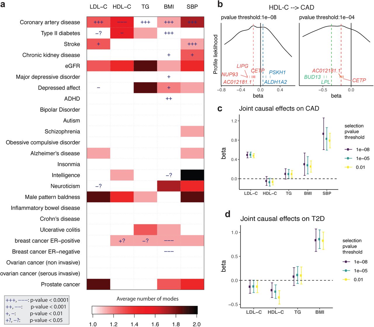
Finally, we apply GRAPPLE to interrogate the causal effects of 5 risk factors on 25 complex diseases through a multivariate genome-wide screen. The five risk factors are three plasma lipid traits: LDL-C, high-density lipoprotein cholesterol (HDL-C), triglycerides (TG), BMI and SBP. The diseases include heart disease, Type II diabetes, kidney disease, common psychiatric disorders, inflammatory disease and cancer (Figure 3a). Though there has been causal effects screening available across traits and risk factors [48, 36, 34], we are the first to look at the landscape of the pleiotropic pathways, which is enabled by mode detection using GRAPPLE. For each pair of the risk factor and disease, we compare across p-value thresholds from 10−8 to 10−2. As a summary of the results, Figure 3a illustrates the average number of modes detected across the p-value thresholds for SNP selection (for modes at each p-value threshold, see Figure S2). Besides the number of modes, Figure 3a also shows the p-values for each risk factor when GRAPPLE is performed with only the single risk factor assuming the “almost random effect” model (see also Figure S2, Methods). These p-values are not valid when there are pleiotropic pathways.
Screening with GRAPPLE. a, Landscape of pleiotropic pathways on 25 diseases. The colors show average number of modes across 7 different selection p-value thresholds. The “+” sign shows a positive estimated effect and “−” sign shows a negative estimated effect, with the p-value for each cell a combined p-value of replicability across 7 thresholds. These p-values are not multiple-testing adjusted across pairs. b, Multi-modality of the profile likelihood for effect of HDL-C on CAD at 2 different selection p-value threshold. Vertical bars are positions of marker SNPs  , labeled by their mapped genes (only unique gene names are shown). c, Multivariate MR with GRAPPLE for the effect of 5 risk factors on CAD. d, Multivariate MR with GRAPPLE for the effect of 4 risk factors on CAD. The Error bars in c and d are 95% confidence intervals.
Figure 3a shows that multi-modality can be detected in many risk factor and disease pairs. Multi-modality is most easily seen using the stringent p-value threshold 10−8 (Figure S2). However, we find that some modes are contributed by a single SNP thus is more likely an outlier than a pathway. For instance, the effect of stroke on LDL-C shows two modes when the p-value threshold is 10−8 or 10−7 (one mode around −2.3 and another mode near 0.08). However, the negative mode only has one marker SNP (rs3184504) which has been found strongly associated with hundreds of different traits according to GWAS Catelog [9] while the other mode has hundreds or marker genes. After removing the SNP rs3184504, the mode disappears. Such a mode also disappears when we increase the p-value threshold to include more SNPs as instruments. Thus, the average number of modes serves as a strength of evidence for the existence of multiple pleiotropic pathways. Some risk factor and disease pairs show multi-modality without having a significant p-value for β, suggesting that the risk factor and disease are genetically correlated through multiple pathways but there is no evidence that risk factor has a causal effect on the disease.
We then focus on two diseases: CAD and T2D. For CAD, all five risk factors show very significant effects, though multi-modality is detected in HDL-C and SBP. First, consider the well-studied, oft-debated relationship between CAD and the lipid traits. In our results for HDL-C, with different p-value thresholds, three modes in total can show up, two being negative and one positive, indicating that the pathways from HDL-C to CAD is complicated (Figure 3b). (Figure 3b shows that one negative mode is contributed by SNPs near genes LPL and BUD13, which are strongly associated with triglycerides. Another positive mode is contributed by SNPs near genes ALDH1A2 and PSKH1, which is related to respiratory diseases [50]. The markers of the other negative mode are mapped to genes including LIPG and CETP.
Since the effects of the lipid traits are generally complicated, we combine all 5 risk factors and run an MR jointly with GRAPPLE (Figure 3c) with different p-value thresholds. After adjusting for other risk factors, the two most prominent risk factors for the heart disease are LDL-C and SBP, while the protective effect of HDL-C stays negligible as well as the risk brought by TG. So these results show that HDL-C as a single measurement does not seem to have a protective effect on heart disease, while there are complicated multiple pathways involved. Researchers have suggested analyzing different subgroups of HDL-C as smaller particles tend to have a stronger protective effect [57].
Lipids are involved in a number of biological functions including energy storage, signaling, and acting as structural components of cell membranes and have been reported to be associated with various diseases [52, 21, 53, 24, 32, 1]. Besides CAD, another disease that most likely involves the lipid traits is the Type II diabetes (Figure 3a). T2D is associated with dyslipidemia (i.e., higher concentrations of TG and LDL-C, and lower concentrations of HDL-C), though the causal relationship is still unclear [20]. In the mean time, evidence has emerged that LDL-C reduction with statin therapy results in a modest increase in risk of T2D [52]. For the MR analyzing each risk factor alone, we see potential protective effects of LDL-C and HDL-C on T2D but also multi-modality patterns. Two modes shows up in the profile likelihood from HDL-C to T2D where one negative mode has a marker gene LPL and a mode near 0 with marker genes CETP and AC012181.1. Thus we include all 3 lipid traits, along with BMI and run a joint model for these 4 risk factors using GRAPPLE (Figure 3d). Our result indicates a mild protective effect of HDL-C on T2D, while showing no enough evidence for the effect of either LDL-C or TG.
3 Discussion
We propose a comprehensive framework that utilizes both strong and weakly associated SNPs to estimate the causal relationship between complex traits. GRAPPLE is robust to pervasive pleiotropy and can identify multiple pleiotropic pathways. The multivariate MR in GRAPPLE can adjust for known confounding risk factors.
GRAPPLE incorporates several improvements over existing MR methods. It gets rid of weak instrument bias by dealing with measurement errors of the SNP effects on exposure with profile likelihood, which is superior to most other methods that can not deal with weak instrument bias. Our likelihood is similar to the models in [12], but we add random effects and robustify the likelihood to make it more realistic under pervasive pleiotropy. The multi-modality visualization shares similarities with [22], which estimates the causal effect by the global mode, but we provide a more comprehensive analysis of multiple pleiotropic pathways. Some recent methods used mixture models to adjusted for pleiotropic pathways, but only allow the existence of one pleiotropic pathway [39, 36, 11, 34]. Our causality direction identification is related to bi-directional MR [49] where if we reverse the role of risk factor and disease, the estimated causal effect is likely to be 0 as the selected IVs would likely to affect the disease through unrelated risk factors. We make this idea visible and tolerate scenarios where IVs affect the disease through risk factors are selected and would bias the conclusion in the reverse MR. Finally, as the intercept term for “directional” pleiotropy in MR-Egger is not invariant to the arbitrary assignment of effect alleles for each SNP, leading to the deficiency of the method, GRAPPLE does not include any intercept term.
GRAPPLE needs a separate GWAS cohort of the exposure for SNP selection, which is necessary for valid inference with weakly associated SNPs. Currently, we find it hard to obtain multiple good-quality public GWAS summary statistics with non-overlapping cohorts. We suggest that the stage-specific or study-specific GWAS data before meta-analysis may be released to the public in the future.
In GRAPPLE, we still require using a p-value threshold, though it can be as mild as 10−2, instead of requiring no p-value threshold at all. There are two main reasons for this requirement. One consideration is to increase power, as including too many SNPs with γj = 0 or extremely small would instead increase the variance of  [56, 55]. Another consideration is that we would not want unmeasured risk factors that are unassociated (or very weakly associated) with target risk factors to bring in large pleiotropic effects on SNPs that mainly affect these unmeasured risk factors. The chance of including these SNPs would be much lower by requiring a mild p-value threshold.
Finally, when discussing the causal effect of a risk factor, one implicit assumption we use is consistency, assuming that there is a clear and only one version of intervention that can be done on the risk factor. However, interventions on risk factors such as BMI are typically vague. For instance, there can be multiple ways to chance weight, such as taking exercise, switching to different diet or conducting a surgery. It is common sense that these different interventions would have different effects on diseases, though they may change BMI by the same amount. Similarly, cholesterol has abundant functions in our body and involve in multiple biological processes. Intervening different biological processes to change the concentrations of lipid traits may also have different effect on diseases. With MR, the interventions are changing risk factors levels with natural mutations, which may be different from interventions with drugs that has a rapid and strong effect on the risk factors. We think that our causal inference using GRAPPLE, along with the markers we detect, would provide abundant information to deeper our understanding of the risk factors. However, one still needs to be careful when giving causal interpretations of the results. One recommendation in practice is to triangulate the results from MR with other sources of evidence [35].
Methods
Model details
The structural equations (1) where X = (X1, X2, …, XK) and β = (β1, β2, …, βK) describe how individual level data are generalized. To link it with the GWAS summary statistics data, denote

Then we can rewrite the structural equations into the following linear models:

 where corr(Zj, ϵjk) = 0 for any k and
  . By replacing X in (6) with (5), we get
 where
where  . As
. As  , we conclude that Γj also satisfies that

Thus, both Γj and γjk represent marginal associations between SNP Zj and the traits of the disease and risk factors, and their relationships follow Equation (2).
When the disease is a binary trait, the structural equation of Y changes to

With the same argument, we have

If we further assume that for each genetic instrument j, Zj is actually independent of ej, then the odds ratio that is estimated from the marginal logistic regression will be approxmately Γj/c with a constant c > 1. In other words, Equation (2) is still approximately correct with the β in (2) a biased (by a ratio of 1/c) version of the β in (7) (for a detailed calculation, see A.1 of [56]).
GWAS summary statistics from overlapping cohorts
The GWAS estimated effect sizes (log odds ratios for binary traits) of SNP j are  for the disease and a length K vector
  for the risk factors. As shown in [7] and derived in SI text without assuming a polygenetic model [8], for any risk factor k we have
 where No and Nek are the total sample sizes for the disease and kth risk factor. Nsk is the number of shared samples. The correlation of Xk and Y of any shared sample is Corr [Ys, Xks]. The standard derivation of
  and
and  are denoted as
  and
and  , which can be considered as known values from the GWAS summary statistics. Equation (8) shows that all the SNPs share the same correlation. As a consequence, we assume
 where Σ is the unknown shared correlation matrix.
Estimate the shared correlation Σ
To estimate Σ from summary statistics, we can use equation (8). We first select unassociated SNPs where γjk = 0 for all risk factors k as the SNPs with their selection p-values pjk ≥ 0.5 for all k.
Denote their Z-values of the estimated effect sizes of both risk factors and disease as matrix ZT×(K+1) where T is the number of selected unassociated SNPs. Then the estimated covariance is ZT Z/T from which we get the estimated correlation matrix.
IV selection using LD clumping
In GRAPPLE, we need to first select a set of independent SNPs as instruments. As shown in [56], the correlations of the estimates  and
and  across independent SNPs are negligible. If the instruments are correlated, stronger assumptions are needed to account for the correlation even when the r2 between any pair of SNPs are “known”. Thus, we only use independent SNPs as instruments to simplify the calculation. Besides the independence requirement, we only include SNPs that pass a p-value threshold. As shown in Figure S1, there is a selection bias if the SNP selection and estimates
  are obtained from the same cohorts or even cohorts with many overlapping samples.
Thus, for each risk factor, we need a separate cohort as the selection cohort that has no-overlapping samples with the risk factor and disease cohorts. If K = 1, the selection p-value is the reported p-values for the SNPs in the selection cohort. For multiple risk factors, the selection p-value is the Bonferroni combined p-values K min(pjk) across the K traits where pjk is the selection p-value of SNP j and trait k. We take the intersection of the SNPs that are measured in all selection, risk factor and disease cohorts as candidate SNPs and use LD clumping with PLINK [26] to select independent SNPs whose selection p-values are smaller than some threshold. The LD r2 threshold is set to 0.001.
Estimate the effects β
Here, we perform statistical analysis with the random effect model αj ∼ N (0, τ 2) for the pleiotropic effects, while robust to outliers where the pleiotropic effects for a few instruments are large.
First, we define for each SNP j the statistics
 where
where  is the variance of
  and
and  is the covariance between
  and
and  in our model (9). Under our assumption, tj(β, τ 2) ∼ 𝒩 (0, 1) at the true value of β and τ for most SNPs. Define the robust profile likelihood as the optimization function
 where ρ(·) is some loss function. By default, GRAPPLE uses the Tukey’s bi-weight loss function. We maximize the robust profile likelihood as well as solving the following estimation equation for the heterogeneity τ 2 which is
 where δ = 𝔼 [ρ(Z)] with Z ∼ 𝒩 (0, 1) following a standard Gaussian distribution. The estimates
  and
and  are obtained using an alternating algorithm: fixing τ 2 to estimate β by maximizing equation (11) and fixing β to estimate τ 2 as the root of Equation (12). It has been shown in our previous work [56] for K = 1 that these estimates are consistent and asymptotically normally distributed when the number of SNPs are large enough. The variance of
  and
and  are further calculated using the delta method with second order Taylor expansions and their confidence intervals can be constructed with these variances. For further mathematical details of the estimation, see SI.
Identify pleiotropic pathways via the multi-modality diagnosis
If there is a confounding Genetic Pathway 2  , as shown in Figure 1a, that are missed, then we have the structural equation
 and also the linear model
 for a SNP j that only associate with Genetic Pathway 2 and uncorrelate with X conditional on
  . Similar to (5), we have

Plug in (13), we have

Thus, if there are enough SNPs like SNP j, they would contribute to another mode of (4) at β + κ/δ.
The same argument works for identification of the causal direction. Say there is another  that affects Y but is uncorrelated with the risk factor X (δ = 0). The existence of such
  is common, unless X is the only heritable risk factor of Y. They would not affect GRAPPLE too much as with a mild p-value threshold on the associate with X, very few SNPs that strongly associate with
  will be selected and GRAPPLE is robust to those outliers. However, SNPs associate with
  can be used to identify the causal direction, as they will have γj = 0 with nonzero Γj that are considerably large. If the role of X and Y are switched, then γj and Γj are also switched. Also, as the selection is now based on the association with Y, a lot of SNPs that associate with
  will be selected and contribute to a mode at 0, while the SNPs that affect Y through X will contribute to a mode at 1/β.
Select marker SNPs and genes for each mode
GRAPPLE uses LD clumping with a stringent r2 (= 0.001) threshold to guanratee independence among the genetic instruments. However, marker SNPs are not restricted to these independent instruments in order to get more biological meaningful markers. Marker SNPs are selected from a SNP set 𝒢 where the SNPs are selected using LD clumping with r2 threshold 0.05.
Assume that there are M modes detected at positions β1, β2, …, βM. Define the residual of SNP j (j ∈ 𝒢) for mode m as
 where tj(·, ·) is defined in Equation (10). SNP j is selected as a marker for mode m if |rjm′| > t1 for any m′ ≠ m and |rjm| ≤ t0. By default, t1 is set to 2 and t0 is set to 1 which gives reasonable results in practice. When the marker SNPs are selected, GRAPPLE further map the SNPs to ENCODE genes where the marker SNPs locate and and search for the traits that these SNPs are strongly associated with in GWA studies by querying HaploReg v4.1 [51] using the R package HaploR. The ratios
  of the marker SNPs are also returned for reference (shown as the vertical bars in Figure 3b).
Compute replicability p-values across SNP selection thresholds
Each p-value shown in Figure 3a summarizes a vector of p-values across 7 different selection p-value thresholds ranging from 10−8 ot 10−2 for each risk factor and disease pair. It reflects how replicable the significance is across SNP selection thresholds. Specifically, it is the partial conjunction p-value [2] for rejecting the null that β is non-zero for at most 2 of the selection thresholds. For a risk factor and disease pair k, let the pvalues computed by using SNPs selected with the 7 thresholds pks where s = 1, 2, …, 7. Then rank them as pk(1) ≤ pk(2) ≤ … ≤ pk(7), the partial conjunction p-value for the pair k is computed as 5pk(3).
Code Availability
The R package GRAPPLE can be installed from Github at https://github.com/jingshuw/GRAPPLE.
Data Availability
All GWAS summary statistics that are used in the analyses of the manuscript are downloaded from public resources, where most of them are downloaded from the GWAS Catelog [9], and the websites of GWAS consortium GIANT, DIAGRAM, PGC, GLGC, and UKBiobank. A complete list of the datasets used in each analysis and where they are from is provided in Supplementary Tables 1 and 2 and Supplementary Note 2. Intermediate results for screening of 5 risk factors on 25 diseases are available at https://www.dropbox.com/sh/myh8xgxne8fo17v/AABWJf781VrCGnqNFMLtnqIea?dl=0.
References
- [1].↵
- [2].↵
- [3].↵
- [4].↵
- [5].↵
- [6].↵
- [7].↵
- [8].↵
- [9].↵
- [10].↵
- [11].↵
- [12].↵
- [13].↵
- [14].↵
- [15].↵
- [16].↵
- [17].↵
- [18].↵
- [19].↵
- [20].↵
- [21].↵
- [22].↵
- [23].↵
- [24].↵
- [25].↵
- [26].↵
- [27].↵
- [28].↵
- [29].↵
- [30].↵
- [31].↵
- [32].↵
- [33].↵
- [34].↵
- [35].↵
- [36].↵
- [37].↵
- [38].↵
- [39].↵
- [40].↵
- [41].↵
- [42].↵
- [43].↵
- [44].↵
- [45].↵
- [46].↵
- [47].↵
- [48].↵
- [49].↵
- [50].↵
- [51].↵
- [52].↵
- [53].↵
- [54].↵
- [55].↵
- [56].↵
- [57].↵


