Task-driven hierarchical deep neural network models of the proprioceptive pathway

Abstract

Biological motor control is versatile and efficient. Muscles are flexible and undergo continuous changes requiring distributed adaptive control mechanisms. How proprioception solves this problem in the brain is unknown. Here we pursue a task-driven modeling approach that has provided important insights into other sensory systems. However, unlike for vision and audition where large annotated datasets of raw images or sound are readily available, data of relevant proprioceptive stimuli are not. We generated a large-scale dataset of human arm trajectories as the hand is tracing the alphabet in 3D space, then using a musculoskeletal model derived the spindle firing rates during these movements. We propose an action recognition task that allows training of hierarchical models to classify the character identity from the spindle firing patterns. Artificial neural networks could robustly solve this task, and the networks’ units show directional movement tuning akin to neurons in the primate somatosensory cortex. The same architectures with random weights also show similar kinematic feature tuning but do not reproduce the diversity of preferred directional tuning nor do they have invariant tuning across 3D space. Taken together our model is the first to link tuning properties in the proprioceptive system to the behavioral level.

Highlights

• We provide a normative approach to derive neural tuning of proprioceptive features from behaviorally-defined objectives.

• We propose a method for creating a scalable muscle spindles dataset based on kinematic data and define an action recognition task as a benchmark.

• Hierarchical neural networks solve the recognition task from muscle spindle inputs.

• Individual neural network units in middle layers resemble neurons in primate somatosensory cortex & make predictions for neurons along the proprioceptive pathway.

Introduction

Proprioception is a critical component of our ability to perform complex movements, localize our body in space and adapt to environmental changes (1–3). Our movements are generated by a large number of muscles and are sensed via a diverse set of receptors, most importantly muscle spindles, which carry highly multiplexed information (2, 4). For instance, arm movements are sensed via distributed and individually ambiguous activity patterns of muscle spindles, which depend on relative joint configurations rather than the absolute hand position (5, 6). Interpreting this high dimensional input (around 50 muscles for a human arm) of distributed information at the relevant behavioral level poses a challenging decoding problem for the central nervous system (6, 7).

Proprioceptive information from the receptors undergoes several processing steps before reaching somatosensory cortex (3, 8) - from the spindles that synapse in Clarke’s nucleus, to cuneate nucleus, thalamus (3, 9), and finally to somatosensory cortex (S1). In cortex, a number of tuning properties have been observed, such as responsiveness to varied combinations of joints and muscle lengths (10, 11), sensitivity to different loads and angles (12), and broad and uni-modal tuning for movement direction during arm movements (11, 13). The proprioceptive information in S1 is then hypothesized to serve as the basis of a wide variety of tasks, via its connections to motor cortex and higher somatosensory processing regions (1–3, 14, 15).

The key role of proprioception is to to sense the state of the body - i.e., its posture and actions (postures over time). This information subserves all other functions from balance to motor learning. Thus, to gain insights into the computations of proprioception, we propose action recognition from peripheral inputs as an objective. Here, we present a framework for studying the proprioceptive pathway using goal-driven modeling combined with a new synthetic dataset of muscle (spindle) activities. Large-scale datasets like ImageNet (16) have allowed training of deep neural networks that can reach (and surpass) human-level accuracy on visual object recognition benchmarks (17, 18). Remarkably, those networks learn image representations that closely resemble tuning properties of single neurons in the ventral pathway of primates and elucidate likely transformations along the ventral stream (17, 19–22). This goal-driven modelling approach (17, 23–25) has since successfully been applied to other sensory modalities such as touch (26, 27), thermosensation (28) and audition (29).

To create a real-world action recognition task, we started from a dataset comprising pen-tip trajectories measured while a human was writing individual single-stroke characters of the Latin alphabet (30). Next, a musculoskeletal model of the human upper limb (31) is employed to generate muscle length configurations corresponding to drawing the pen-tip trajectories in multiple horizontal and vertical planes. These are finally converted into spindle firing rates using a model of spindle activity (32). We then used this proprioceptive ‘action recognition’ task to train neural networks to recognize hand-written characters from the modeled spindle firing rates. Through an extensive hyper-parameter search we found neural network architectures that optimally solve the task. We then examine to what extent training influences representation by comparing the coding in both untrained and trained networks. We identify individual units in the network’s middle layers that display kinematic coding similar to that found in numerous biological experiments in both the trained and control networks, but also find high-level kinematic tuning properties that are only present in the trained networks. We believe our study outlines a fruitful approach to model the proprioceptive system.

Results

Spindle-based biomechanical character recognition task

In order to model the proprioceptive system in a goal-driven way, we designed a real-world proprioceptive task. The objective is to classify the identity of Latin alphabet characters based on the proprioceptive inputs that arise from the simulated activity of muscle spindles, when the arm is passively moved (Figure 1). In order to create this dataset, we started from the 20 characters that can be handwritten in a single stroke (thus excluding f, i, j, k, t and x, which are multi-stroke) using a dataset of pen-tip trajectories (30, 33). Then we generated 1 million end-effector (hand) trajectories by scaling, rotating, shearing, translating and varying the speed of each original trajectory (Figure 2A-C; Table 1). As we did not model the muscles of the hand itself the location of the end-effector is taken to be the hand location.

Table 1.

Variable range for the utilized data augmentation applied to the original pen-tip trajectory dataset. Furthermore, the character trajectories are translated to start at various starting points throughout the arm’s workspace. Overall yielding movements in 26 horizontal and 18 vertical planes.

Figure 1. Spindle-based biomechanical character recognition task to elucidate proprioception:

Muscle spindle firing rates that correspond to the tracing of individual letters were simulated using a musculoskeletal model of a human arm (actions). This scalable action recognition dataset can then be used to train deep neural networks models of the proprioceptive pathway to classify the characters based on the input muscle spindle firing rates. One can then analyze these models and compare and contrast them with what is known about the proprioceptive system in primates.

Figure 2. The proprioceptive character recognition dataset generation.

(A) Multiple example pen-tip trajectories for five of the 20 letters are shown. (B) Same trajectories as in A, plotted as time courses of Cartesian coordinates. (C) Creating (hand) end-effector trajectories from pen-tip trajectories. (left) An example trajectory of character ‘a’ resized to fit in a 10cm x 10cm grid, linearly interpolated from the true trajectory while maintaining true velocity profile. (right) This trajectory is further transformed by scaling, rotating and varying its speed. (D) Candidate starting points to write the character in space. (left) A 2-link 4 degree of freedom (DoF) model human arm is used to randomly select several candidate starting points in the workspace of the arm (right), such that written characters are all strictly reachable by the arm. (E) (left to right) Given a sample trajectory in C and a starting point in the arm’s work-space, the trajectory is then drawn on either a vertical or horizontal plane that passes through the starting point. We then apply inverse kinematics to solve for the joint angles required to produce the traced trajectory. (F) (left to right): The joint angles obtained in E are used to drive a musculoskeletal model of the human arm in OpenSim, to obtain equilibrium muscle fiber-length trajectories of 25 relevant upper arm muscles. These muscle fiber-lengths are transformed into muscle spindle Ia firing rates using a spindle model. Mean subtracted firing rate profiles are shown.

To translate end-effector trajectories into 3D arm movements we computed the joint-angle trajectories through inverse kinematics using a constrained optimization approach (Figure 2D-E). We iteratively constrain the solution space by choosing joint angles in vicinity of the previous configuration in order to eliminate redundancy. To cover a large 3D workspace we placed the characters in multiple horizontal (26) and vertical (18) planes and calculated corresponding joint-angle trajectories (starting points are shown in Figure 2D). From this set, we selected a subset of two hundred thousand examples with smooth, non-jerky muscle length changes, while making sure that the set is balanced in terms of the number of examples per class (see Methods). A human upper-limb model in OpenSim (31) was then used to compute equilibrium muscle lengths for 25 muscles in the upper arm that lead to the corresponding joint angle trajectory (Figure 2F, Suppl. Video 1). Based on these simulations, we generated muscle spindle Ia primary afferent firing rates using a model proposed by Prochazka-Gorassini (32) that is devoid of positional information - allowing us to isolate the effect of velocity encoding (actions) only. To simulate neural variability, we added Gaussian noise to the simulated muscle length trajectories and spindle firing rates (Figure 2F). Since not all characters take the same amount of time to write, we padded the movements with static postures corresponding to the starting and ending postures of the movement and randomized the initiation of the movement in order to maintain ambiguity about when the writing begins. At the end of this process each sample consists of simulated spindle Ia firing rates from each of the 25 muscles over a period of 4.8 seconds, simulated at 66.7 Hz. The dataset was split into a training, validation and test set with a 72-8-20 ratio.

Recognizing characters from spindles is challenging

We reasoned that several factors complicate the recognition of a specific character: Firstly, the end-effector position is only present as a distributed pattern of muscle spindle activity; secondly, the same character will give rise to widely different spindle inputs depending on different arm configurations. Our dataset allowed us to directly test how these aspects affected performance. Namely, we could test if the direct input (spindle firing), joint angles, and/or position of the end-effector influenced the difficultly of the task.

To begin, we visualized the data at the level of the spindle firing activity by using t-distributed stochastic neighbor embedding (t-SNE, 34). This illustrated that the data was entangled (Figure 3A). To quantify the separability we trained linear, multi-class support vector machines (SVM, 35). The performance of this decoder, which received the entire 4.8 seconds of the trajectories as regressors, was poor regardless of whether or not the input was end-effector coordinates, joint angles, normalized muscle lengths, or spindle firing rates (Figure 3B; see “All”). In fact, the action recognition accuracy was worst for muscle spindle Ia firing rates (≈23%) likely due to the added noise and augmentation. An additional analysis with less variability was performed by suppressing some of the augmentations (scale, plane, and speed). As expected, performance increased with moderately decreasing variability (Figure 3B). Taken together, these analyses suggest that at the level of the afferent fibers it is difficult to extract the character class. To further illustrate this we directly compared specific characters by performing pairwise SVM classification. Here, the influence of the specific geometry of each character is notable. On average the pairwise accuracy is 81.5±14.1 (mean ± S.D., N = 190 pairs, Figure 3C). As expected, similar looking characters are harder to distinguish at the level of spindles - i.e. “e” and “y” were easily distinguishable but “m” and “w” were not (Figure 3C). Collectively, we demonstrated that the proposed task is challenging as illustrated by t-SNE embedding (Figure 3A) and quantified by SVM performance (Figure 3B, C).

Figure 3. Quantifying character recognition task performance.

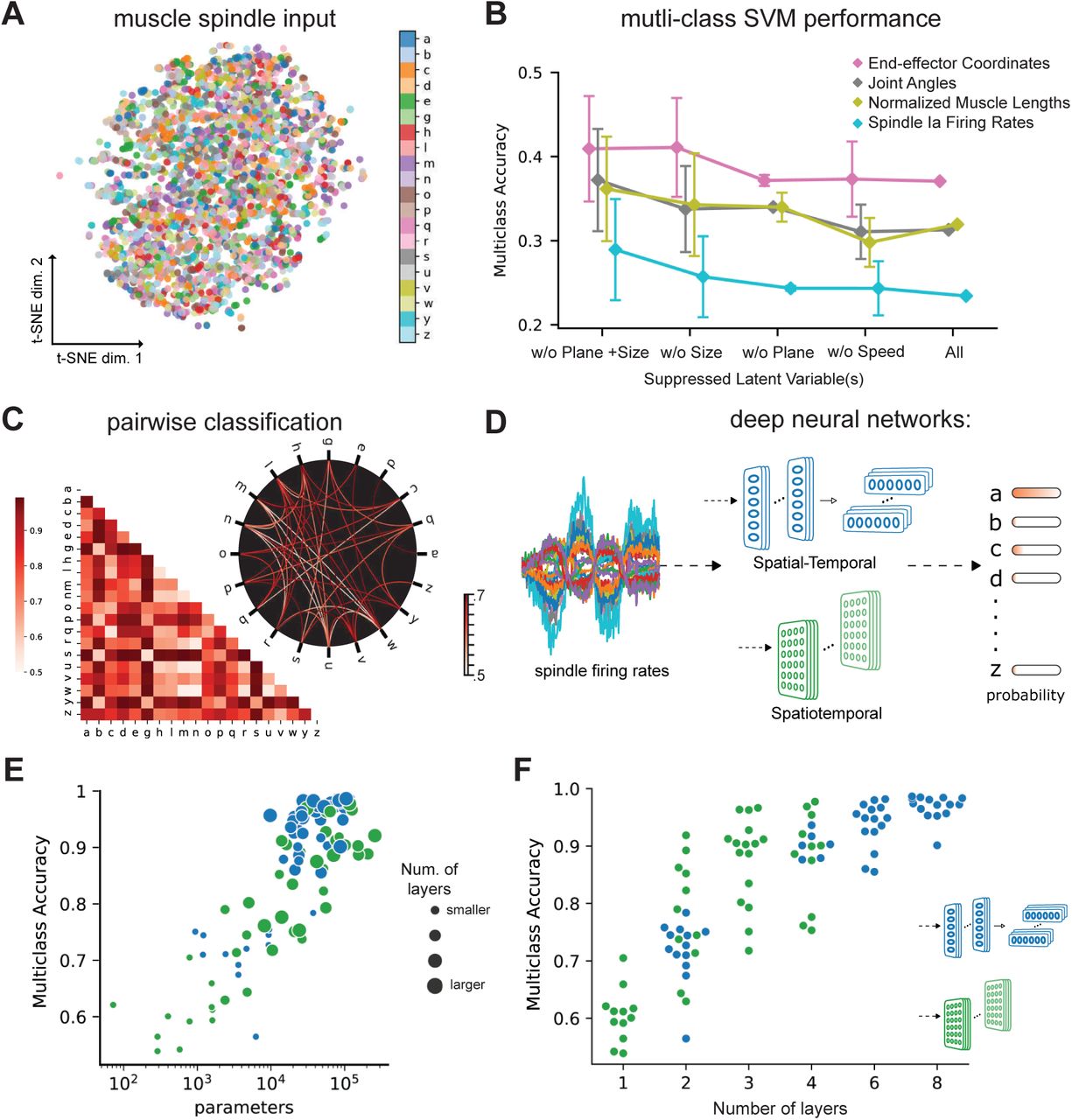
(A) t-SNE embedding of the muscle spindle inputs. (B) Multi-class SVM performance computed using a one-vs-one strategy for different types of input/kinematic representations. To gain insight into the role of augmentation we suppressed various latent variables, different splits of the dataset were used to generate each individual point, where one or more latent variables used to generate the original dataset were suppressed. Each point denotes mean ± SEM classification accuracy, where N refers to the amount of subsets with fixed latent variables (see Methods). (C) Classification performance for all pairs of characters with a binary SVM given spindle firing rates. Chance level accuracy=50%. The pairwise accuracy is 81.5±14.1% (mean±S.D., N = 190 pairs). Subset of data is also illustrated as circular graph, edge color denotes the classification accuracy. For clarity only pairs with performance less than 70% is shown, which corresponds to the bottom 24% of all pairs. (D) Neural networks are trained on a proprioceptive character recognition task based on noisy muscle spindle input. We tested two neural network architecture families. Each model is comprised of one or more processing layers as shown here. Processing of spatial and temporal information takes place through a series of 1-D or 2-D convolutional layers. (E) Test performance of 50 networks of each type is plotted against the number of convolutional parameters of the networks. (F) Test performance for each network is plotted against the number of layers of the network (N = 50 per model type).

Neural networks models of proprioception

We defined families of artificial neural network models (ANNs) to potentially solve this proprioceptive character recognition task. ANNs are powerful models for both their performance and for elucidating neural representations and computations. An ANN consists of layers of simplified units (“neurons”) whose connectivity patterns mimic the hierarchical, integrative properties of biological neurons and anatomical pathways (17, 23, 36). As candidate models, we parameterized two different kinds of convolutional neural networks (CNNs 37), which impose different inductive priors on the computations in the proprioceptive processing system. We refer to these families as spatial-temporal and spatiotemporal networks (Figure 3D). Importantly, they differ in the way they integrate spatial and temporal information along the hierarchy. These two types of information can be processed either sequentially, as is the case for the spatial-temporal network type that contains layers with one-dimensional filters that first integrate information across the different muscles, followed by an equal number of layers that integrate only in the temporal direction or simultaneously, using two-dimensional kernels, as they are in the spatiotemporal network. Within each model family, candidate models can be created by varying hyper-parameters such as the number of layers, number and size of spatial and temporal filters, type of regularization and response normalization, among others (see Methods). As a first step to restrict the number of models, we performed a hyper-parameter architecture search by selecting models according to their performance on the character recognition task. We should emphasize that our ANNs are simultaneously integrating spindles and time, unlike standard feedforward CNN-models of the visual pathway that just operate on images. The type of architectures we used are also called Temporal Convolutional Networks (TCN); they have been shown to be excellent for time series modeling and often outperform recurrent neural networks (38). TCNs also naturally describe neurons along a sensory pathway that integrate spatio-temporal inputs, which motivated us to use such architectures.

Architecture search & representational changes

To find models that could solve the character recognition task, we performed an architecture search and trained 100 models (50 models from each network type, see Table 2). Weights were trained using the Adam optimizer (39) until performance on the validation set saturated. After training, all models were evaluated on a dedicated test set (see Methods; Figure S1A, B).

Figure S1. Network Performance.

(A) Training vs. test performance for all networks. Shallower networks tend to overfit more. (B) Performance of 50 networks of each type is plotted against the all parameters of the networks. Unlike Figure 3F this figure also counts the parameters of the dense output layer, which is dominated by the number of dimensions of the tensor at the last convolutional layer.

Table 2.

Hyper-parameters for neural network architecture search. Left: Possible parameter choices for the two network types. First, a number of layers (per type) is chosen, ranging from 2-8 (in multiples of 2) for spatial-temporal models and 1-4 for the spatiotemporal ones. Next, a spatial and temporal kernel size per Layer (pL) is picked, which remains unchanged throughout the network. For the spatiotemporal model, the kernel size is equal in both the spatial and temporal directions in each layer. Then, for each layer, an associated number of kernels/feature maps is chosen such that it never decreases along the hierarchy. Finally, a spatial and temporal stride is chosen. All parameters are randomized independently and 50 models are sampled per network type. right: Parameter choices for the 2 top-performing models. The values given under the “spatial” rows count for both the spatial and temporal directions for the spatiotemporal model.

Models of both types could solve the task (98.60% ±0.02, Mean ± SEM for the best spatial-temporal model, and 97.81% ± 0.06 for the best spatiotemporal model, N = 5 instantiations; Figure 3E). Of the model hyper-parameters considered, depth of the networks influenced performance the most (Figure 3F). The parameters of the best performing architectures are displayed in Table 2. Having found models that robustly solve the character recognition task, we sought to analyze their properties. We created five pretraining (control) post-training (trained) pairs of models for the best-performing model architecture (per type) for further analysis. We will refer to those as “instantiations”. As expected, the randomly initialized models performed at chance level (spatial-temporal: 5.01% ± 0.04, spatiotemporal: 4.92% ± 0.07, Mean ± SEM, N = 5).

How did the population activity change across the layers after learning the task? We first compared the representations across different layers for each trained model to its random initialization by linear Centered Kernel Alignment (see Methods). This analysis revealed that for all instantiations the representations remained highly similar between the trained and control models for the first few layers and then deviate in the middle to final layers of the network (Figure 4A). Therefore, we found that learning substantially changes the representations. Next, we aimed to understand how the task is solved, i.e., how the different stimuli are transformed across the hierarchy.

Figure 4. Low-dimensional embedding of network layers reveals structure.

(A) Similarity in representations (CKA) between the trained and the control models for each of the five instantiations per model type. (B) t-distributed stochastic neighbor embedding (t-SNE) for each layer of an example spatial-temporal model. Each data point is a random stimulus sample (N = 2, 000, 50 per stimulus). (C) Representational Dissimilarity Matrices (RDM). Character level representation are calculated through percentile representational dissimilarity matrices for muscle spindle inputs and final layer features of the two best ANN networks. (D) Similarity in stimulus representations between representational dissimilarity matrices of an ideal observer and each layer for the five instantiations (faint lines) as well as their means (solid lines) of the two best trained models and their controls.

Untangling stimuli to classes

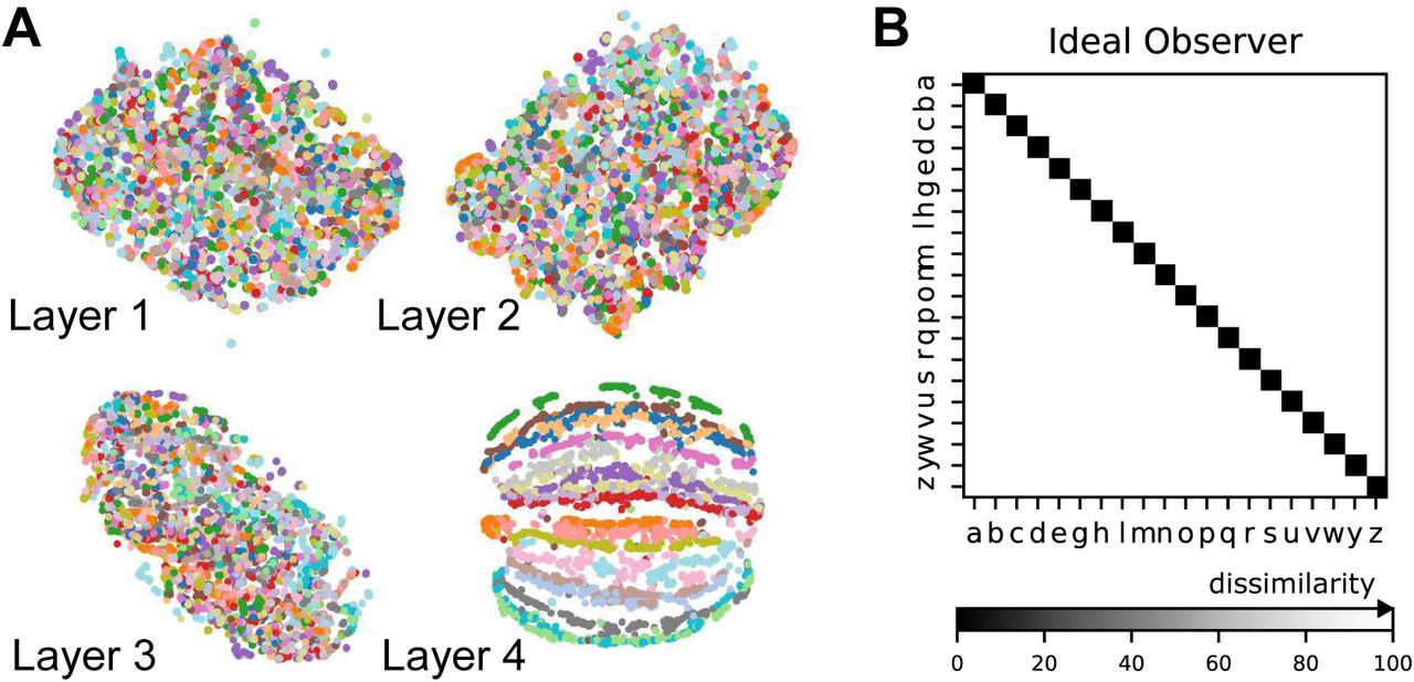
First, we wanted to illustrate the geometry of the ANN representations and how the different characters are disentangled across the hierarchy. We started by using t-SNE to display the structure. In these representations the different characters remain entangled throughout most of the processing hierarchy, before finally separating in the final layers (spatial-temporal model: Figure 4B, spatiotemporal model: Figure S2A). In order to quantify this, we then computed representational dissimilarity matrices (RDM; see Methods). We found that different instances for the same characters were not represented similarly at the level of muscle spindle firing rates, but at level of the last convolutional layer for the trained models (Figure 4C. An ideal observer would have a block structure, with correlation 1 for all stimuli of the same class and 0 otherwise (Figure S2B). To quantify how the characters are represented across the hierarchy, we computed the similarity to the ideal observer’s RDM and found for all the models the similarity only increased towards the last layers (Figure 4D). This finding corroborates the visual impression from Figures 4C, S2B that different characters are disentangled near the end of the processing hierarchy. Having found that characters are not immediately separable, we next wanted to identify what variables were encoded in single units.

Figure S2. t-SNE embedding for the spatiotemporal model.

(A) T-distributed stochastic neighbor embedding (t-SNE) embedding for each layer of the best spatiotemporal model. Each data point is a random stimulus sample (N=4,000, 200 per character). (B) RDM of an ideal observer, which has low dissimilarity for different samples of the same character and high dissimilarity for different samples of different characters.

Single unit tuning properties

We will first consider task variables like class tuning and then look specifically for tuning curves as they have been described in the primate literature (3, 13). Given that the network’s task is to classify the characters, we asked if single units are well tuned for specific characters. To test this we trained an SVM to classify characters from the single unit activations. Even in the final layer (before the readout) of the spatial-temporal model, the median classification performance over the five model instantiations as measured by the normalized area under the ROC curve-based selectivity index for single units was 0.110±0.002 (mean ± SEM, N = 5), and was never higher than 0.31 for any individual unit across all model instantiations (see Methods). Thus, even in the final layer there are effectively no single-character specific units. Of course, combining the different units of the final fully connected layer gives a high fidelity readout of the character and allows the model to achieve high classification accuracy. Thus, character identity is represented in a distributed way.

Position, direction, velocity, and acceleration tuning

What information is encoded in single units? Are tuning features found in biological proprioceptive systems (3, 13) present in the networks? Specifically, we analyzed the units for end-effector position, velocity, direction, coupled direction and velocity, and acceleration tuning. We performed these analyses by relating variables (such as movement direction) to the activity of single units during the continuous movement (see Methods). Units with a test-R² > 0.2 were considered “tuned” to that feature.

Units in both the trained and control models were poorly tuned for end-effector position in both Cartesian and polar coordinate frames, i.e., no units had R² > 0.2 (see Methods, Figure S3). This is likely both a function of the task, as absolute position does not explicitly help to solve it due to the data augmentation, and the fact that the inputs to our model are invariant to absolute position but respond to changes in muscle length.

Figure S3. Positional tuning of single neurons.

(A) For an example instantiation, the distribution of test R² scores for both the trained and control model are shown, for positional tuning (in Cartesian and polar coordinates). The units are not tuned to position. Note that in layer 8 a few units of the control model had a coefficient of determination of 1 as they are constant. (B) Same as A but for the spatiotemporal model.

Next we focused on direction tuning in all horizontal planes. We fit directional tuning curves to the units with respect to the instantaneous movement direction. Spindle Ia afferents, including the model we used (32), are known to be tuned to motion, i.e. velocity and direction. We verified that most Ia spindle afferents had high tuning scores for direction (median R² = 0.66, N = 25) and direction and velocity (median R² = 0.77, N = 25) given the movement statistics (Figure 5A-C). Directional tuning was prominent in middle layers 1-5 before decreasing by layer 8, and large fractions of units exhibited tuning to many kinematic variables with R² > 0.2 (Figure 5C, D). This evolution can also be observed for the typical units shown (Figure 5A, B). However, tuned units were not unique to the trained models. Remarkably, kinematic tuning for the corresponding control model was of a comparable magnitude when looking at the distribution R² scores (Figure 5D). This observation is further corroborated, when comparing the 90%-quantiles for all the instantiations (Figure 5E). These findings revealed that the trained and control models have similar tuning properties and we wondered, if clearly different signatures exist.

Figure 5. Analysis of single unit tuning properties for spatial-temporal models.

(A) Polar scatter plots showing the activation of units (radius r) as a function of end-effector direction as represented by the angle θ for directionally tuned units. Directions correspond to that of the end-effector while tracing characters in the model workspace. The activation strengths of one muscle spindle, one unit in layer 4 and 8 of the are shown. (B) Similar to A, except that now radius describes velocity, and color represents activation strength. The contours are determined following linear interpolation, with gaps filled in by neighbor interpolation, and results smoothed using a Gaussian filter. Examples of one muscle spindle, one unit in layer 3, 5 and 8 are shown. (C) For each layer of one trained instantiation, the units are classified into types based on their tuning. A unit was classified as belonging to a particular type if its tuning had a test R² > 0.2. Tested features were direction tuning, velocity tuning, acceleration tuning, and label tuning. Conjunctive categorization is possible. (D) For an example instantiation, the distribution of test R² scores for both the trained and control model are shown, for five kinds of kinematic tuning for each layer: direction-only tuning, velocity-only tuning, direction and velocity tuning, acceleration tuning, and label-specificity. The solid line connects the 90%-quantiles of two of the tuning curve types, direction tuning (dark) and acceleration tuning (light). (E) The means of 90%-quantiles over all five model instantiations of trained and control models are shown for direction tuning (dark) and acceleration tuning (light). 95%-confidence intervals are shown over instantiations (N = 5).

Uniformity and coding invariance

We reasoned that in order to solve the task the units learn to represent the input in a distributed manner. To test this we scrutinized the distributions of preferred directions and whether coding properties that are invariant across different workspaces.

Prud’homme and Kalaska found a relatively uniform distribution of preferred directions in primate S1 during a center out reaching 2D manipulandum-based task (Figure 6A from (13)). In contrast, most spindle Ia afferent have preferred directions located along one major axis pointing frontally and slightly away from the body (Figure 6B). Qualitatively, it appears that the trained model had more uniformly distributed preferred directions in the middle layers compared to control models (Figure 6C). To quantify this, we calculated the total absolute deviation (TAD) from uniformity in the distribution of preferred directions. The results indicate that the distribution of preferred directions becomes more uniform in middle layers for all instantiations of the spatial-temporal model (Figure 6D). Indeed layers 4-6 have significantly different TADs (layer 4 t(4) = −5.48, p=0.005, layer 5 t(4) = −4.60, p=0.01, layer 6 t(4) = −11.54, p=0.0003; paired t-test). Thus, learning indeed changes the tuning properties at the population level.

Figure 6. Distribution of preferred directions and invariance of representation across workspaces.

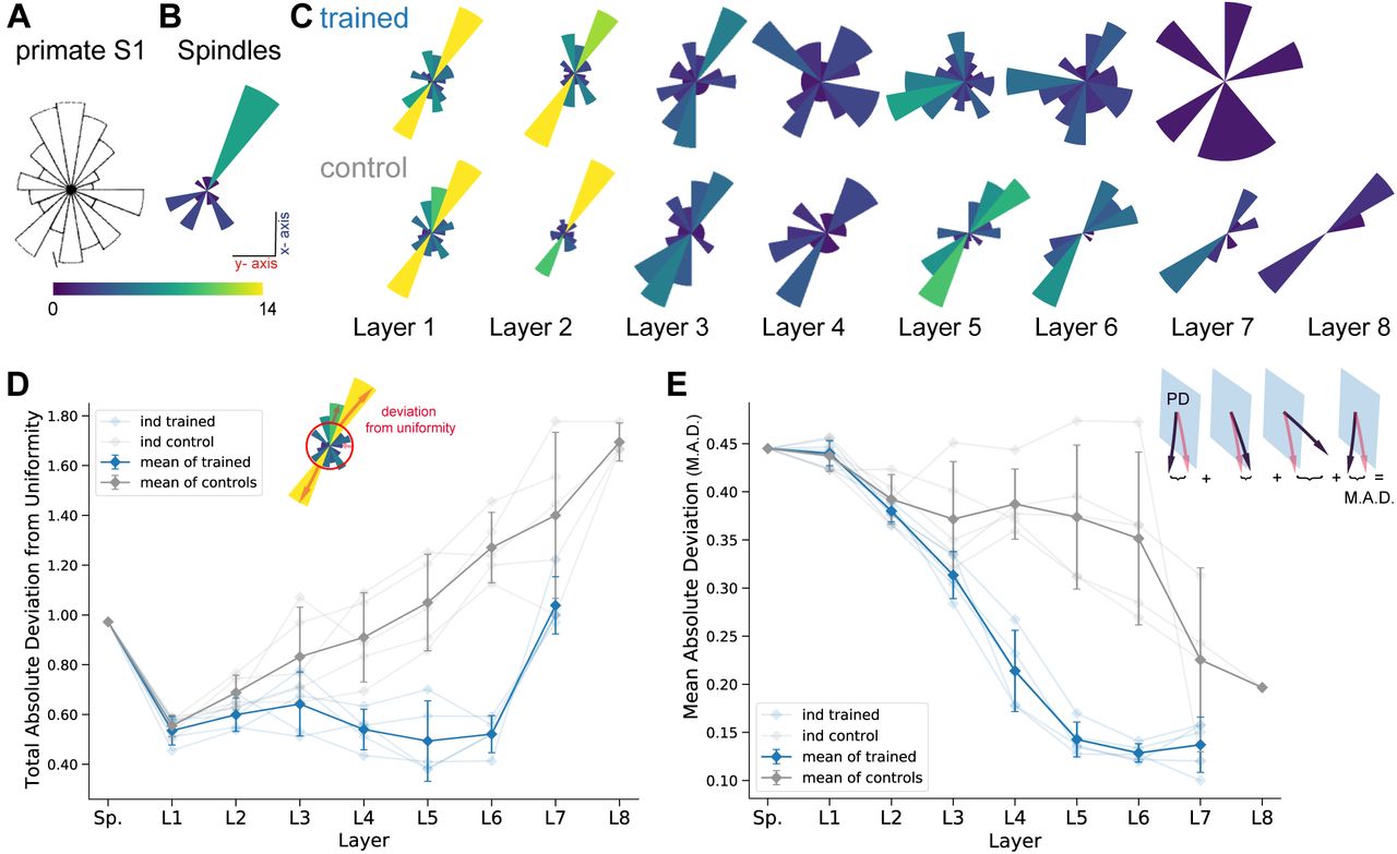
(A) Adopted from (13); distribution of preferred directions in primate S1. (B) Distribution of preferred directions for spindle input. (C) Distribution of preferred directions for one spatial-temporal model instantiation (all units with R² > 0.2 are included). Bottom: the corresponding control. For visibility all histograms are scaled to the same size and the colors indicate the number of tuned neurons. (D) For quantifying uniformity, we calculated the total absolute deviation from the corresponding uniform distribution over the bins in the histogram (red line in inset). Normalized absolute deviation from uniform distribution for preferred directions per instantiation (N = 5, faint lines) for trained and control models as well as mean and 95%-confidence intervals over instantiations (solid line; N = 5). Note that there is no data for layer 8 of the trained spatial-temporal model, as it has no direction selective units (R² > 0.2). (E) For quantifying invariance we calculated mean absolute deviation in preferred orientation for units from the central plane to each other vertical plane (for units with R² > 0.2). Results are shown for each instantiation (N = 5, faint lines) for trained and control models plus mean (solid) and 95%-confidence intervals over instantiations (N = 5). Note that several instantiations for layer 8 had fewer than three directionally tuned units in all planes and were therefore excluded.

As part of creating the large-scale dataset we performed augmentation by having the characters traced in multiple vertical and horizontal planes. Therefore, we could directly test if preferred tuning directions (of tuned units) were maintained across different planes. We hypothesized that for the trained networks preferred orientations would be more preserved across planes compared to controls. In order to examine how an individual unit’s preferred direction changed across different planes, directional tuning curve models were fit in each horizontal/vertical plane separately (examples in Figure S4A, B). To measure the representational invariance, we took the mean absolute deviation (MAD) of the preferred tuning direction for directionally tuned units (R² > 0.2) across planes (see Methods) and averaged over all planes (Figures 6E, S4C). For the spatial-temporal model across vertical workspaces, layers 4-6 were indeed more invariant in their preferred directions (layer 4: t(4) = −10.06, p=0.0005; layer 5: t(4) = −7.69, p=0.002; layer 6: t(4) = −6.19, p=0.0035; Figure 6E), but not for the horizontal planes (Figure S4C). This may stem from the larger invariance of spindles across different horizontal (MAD: 0.272 ± 0.006, mean ± SEM, N = 25) but not vertical workspaces (MAD: 0.485 ± 0.025, mean ± SEM, N = 16; Figure S4A).

Figure S4. Invariance of preferred orientations.

(A) Deviation in preferred direction for individual spindles (N=25). The preferred directions are fit for each plane and displayed in relation to a central horizontal (left) and vertical plane (right). Individual gray lines are for all units (spindles) with R² > 0.2, the thick red line marks the mean. (B) Same as A, but for direction tuning in vertical planes for units in layer 5 of one instantiation of the best spatial-temporal model for the trained (left) and control model (right). Individual gray lines are for units with R² > 0.2, and the red line is the plane-wise mean. (C) Quantification of invariance: Changes in preferred direction across different work spaces (horizontal planes). Mean absolute deviation in preferred orientation of a unit from the central plane to each other horizontal plane (for unit’s with R² > 0). Results for each instantiation (n = 5, faint lines) for trained and control models as well as as mean and 95%-confidence intervals over instantiations (solid line; N=5) are shown. Results are shown for all trained and control model instantiations for the best spatial-temporal (left) and spatiotemporal (right) models. Unlike for the vertical direction, the difference is not statistically significant in the intermediate layers for either the spatial temporal model (layer 4: t(4) = −1.28, p=0.27; layer 5: t(4) = −0.32, p=0.76; layer 6: t(4) = −1.92, p=0.13; layer 7: t(4) = −0.73, p =0.51) or the spatiotemporal model (layer 2: t(4) = 1.55, p=0.20; layer 3: t(4) = 1.61, p=0.18). Note that there is no data for layer 8 of the spatial-temporal and layer 4 of the spatiotemporal trained models, as these had fewer than three direction selective units in all planes (R² > 0.2).

Results for the best spatiotemporal model

As we initially found that the spatiotemporal model also solved the task, we analyzed the changes in the layers in this variant of control vs. trained networks (Figure S5). This model is of equal interest because each unit simultaneously processes patterns across time and muscle channels, which is perhaps more biologically plausible. Importantly, the results corroborate the salient results we found for the spatial-temporal model. We find highly similar “biological” tuning across the layers (Figure S5A). The middle layer displays more uniformly distributed preferred tuning in horizontal planes (Figure S5B). There is a significant divergence in total absolute deviation (TAD) from uniformity for trained vs. controls in the middle layers (layer 2: t(4) = −4.351, p=0.0121; layer 3: t(4) = −4.345, p=0.0122; Figure S5C). Furthermore, as for the spatial-temporal model, the trained networks vs. control models had more invariant tuning across vertical workspaces (layer 2: t(4) = −5.40, p=0.0057; layer 3: t(4) = −5.32, p=0.0060; Figure S5D) but not horizontal workspaces (Figure S4C).

Figure S5. Results for the spatiotemporal models.

(A) For an example instantiation, the distribution of test R² scores for both the trained and control model are shown for five kinds of kinematic tuning for each layer: direction-only tuning, velocity-only tuning, direction and velocity tuning, acceleration tuning, and label-specificity. The solid line connects the 90%-quantiles of two of the tuning curve types, direction tuning (dark) and acceleration tuning (light). (B) Distribution of preferred directions of layer 1 and layer 2 for a spatiotemporal model instantiation from A (all R² > 0.2 neurons are included). (C) Quantification of uniformity as in Figure 6D but for the spatiotemporal model. Faint lines represent a model instantiation, dark lines show mean and confidence intervals (N=5). Note that there is no data for layer 4 of the trained model, as it has no direction selective units (R² > 0.2). (D) Quantification of invariance as in Figure 6E but for the spatiotemporal model. Faint lines represent a model instantiation, dark lines show mean and confidence intervals (N=5). Note that there is no data for layer 4 of the trained model, as it has no direction selective units (R² > 0.2).

Figure S6. Supplementary Video

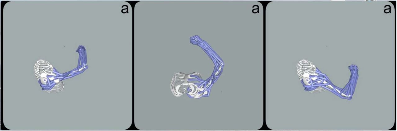
Video depicts the OpenSim model being passively moved to match the human-drawn character “a” for three different variants; drawn vertically (left, right) and horizontally (middle).

In the spatiotemporal models, in which both spatial and temporal filtering occurs between all layers, we observe a monotonic decrease in the fraction of directional tuning across the four layers (Figure S5A). In contrast, across the first four layers fraction of directional tuning is stable and decreases from layer 4-8 in the spatial-temporal model (Figure 5E). This difference is perhaps also expected as the temporal processing implies that a given time point the model receives information from multiple past arm positions (via the spindles). Thus, the correlation to the instantaneous features like velocity degrades “faster” compared to the spatial-temporal model that processes spatial and only then temporal information serially.

Discussion

Task-Driven Modeling of Proprioception

We presented a task-driven approach to study the proprioceptive system. We created a passive character recognition task for a simulated human biomechanical arm paired with a muscle spindle model and found that deep neural networks can be trained to accurately solve the character recognition task. The depth of the networks influenced performance (Figure 3B), similar to what was found for deep task-constrained models of the rodent barrel cortex (26) and is known for object recognition performance on ImageNet (18, 21). Inferring the character from passive arm traces was chosen as it is a type of task that humans can easily perform and because it covers a wide range of natural movements of the arm. The perception is also likely fast, so that feed-forward processing is a good approximation. Additionally, character recognition is an influential task for studying ANNs, for instance MNIST (37, 40). Moreover, when writing movements were imposed onto the ankle with a fixed knee joint, the movement trajectory could be decoded from a few spindles using a population vector model, suggesting that spindle information is accurate enough for decoding (41). Lastly, while the underlying movements are natural and of ethological importance for humans, the task itself is only a small subset of human upper-limb function. Thus, it posed an interesting question whether such a task would be sufficient to induce representations similar to biological neurons.

We found that a large fraction of neurons have direction selective tuning curves (Figure 5 and S5). However, unlike for typical studies of the visual system (e.g. 17, 19, 20, 22), we did not start from ‘raw’ images, but used musculoskeletal and spindle models to turn the raw end-effector trajectories into muscle receptor inputs. There are some notable exceptions that model the visual system while including a model of the retina (42). We believe that imposing known physical and biological constraints allows for a more realistic study of the corresponding nervous system. Spindle Ia afferents were used as the input to the proprioceptive system model, and in particular a highly simplified model proposed by Prochazka-Gorassini (32). We used this model as it is computationally more tractable for large-scale data than alternative models of spindles (43, 44). We decided to include only one type for this study to be able to isolate the fibers that respond to muscle length, namely the fast-adapting spindle Ia afferents, to see if realistic kinematic features emerged.

For the emergence of kinematic tuning, task-driven optimization of the network was not important, while uniformity and invariance only arose after optimizing the network weights on the task. The distribution of preferred directions becomes more uniform over the course of the processing hierarchy (Figure 6), similar to the distribution of preferred tuning in somatosensory cortex (13). This does not occur in the randomized control, which instead maintained an input distribution centered on the primary axis of preferred directions of the muscular tuning curves. This could be a correlate of sensorimotor learning: Since the network is trained to discriminate between different characters, neurons that are tuned to all different directions instead of just one primary axis could allow for an easier differentiation of characters whose traces are quite similar along the muscle spindles’ preferred axis but different otherwise. Furthermore, the models make a prediction about the distribution of preferred directions along the proprioceptive pathway. For instance, we predict that in “lower” layers in the propriocetive biological system, i.e. brainstem, cuneate nucleus, preferred directions are likely to be aligned along major axes inherited from muscle spindles that correspond to biomechanical constraints. Another higher-order feature we considered, was tuning invariance across different workspaces (Figure 6E, Figure S5D). We found that even controls have similar distributions of directionally tuned neurons, which suggests that this feature is simply inherited from muscle spindles. In our computational study, we could probe many different workspaces (26 horizontal and 18 vertical) to reveal that character recognition alone can make tuning more invariant. This highlights the importance of sampling the movement space well, as also emphasized by pioneering experimental studies (45).

Trained vs. controls: what insights we can gain

The comparison with the control networks deserves further attention. Despite the numerous studies on task-driven modeling that have been conducted in the past (19, 21, 22, 26, 29), the only other example we know of in which a similar analysis has been performed was by Cadena et al.(46) (and along different lines 20). Cadena et al. showed that models with randomized weights could predict neural responses in four key visual areas in mice as well as ImageNet pretrained models. Ultimately, the appeal of task-driven modeling comes from the belief that convergent evolution and the mechanistic task-constraints will force a neural network to develop the same representations as the biological system (17, 23). This idea is challenged for those tuning features that models with random weights also develop. As such, Cadena’s and our study both provide a cautionary tale for (over-) interpreting tuning curves in the absence of controls. It is worth noting, however, that especially in Cadena’s study (but to a lesser degree also ours), the weights were randomized for a model architecture that had undergone rigorous optimization (VGG16). This might partially explain the high degree of tuning for kinematic as a consequence of architecture and input statistics. The fact that the architecture alone can determine so much of the tuning follows an interesting parallel development in machine learning, namely, the development of weight agnostic neural networks (47) and the observation that untrained CNNs are remarkably powerful for many image processing problems (48). Although this effect has not been studied explicitly, the difference in kinematic tuning strengths between the top performing models of the spatial-temporal and spatiotemporal types in our study provide first evidence for the importance of architecture.

Informing biological studies

Deep learning can inform theories of the brain (23, 24), cf. (25). Firstly, feed-forward neural networks have contributed to our understanding of sensory systems such as vision (17, 20, 22), touch (26, 27), thermosensation (28), audition (29) and our work adds proprioception, as studied by an action recognition task, to this list. For the motor system as well as cognition, recurrent models have also been applied. Banino et al. trained a recurrent neural network (RNN) to perform path integration, leading to the emergence of grid cells (49). Sussillo et al. showed that regularized RNNs that are trained to reproduce EMG signals learn transient signals that are reminiscent of motor cortical activity (50). Michaels et al. combined CNNs and RNNs to build a model for visually guided reaching (51). Lilicrap and Scott assumed that neural activity in motor cortex is optimized for controlling the biomechanics of the limb and they could explain the non-uniform distribution of tuning directions in motor neurons (52). Furthermore, they argued that biases are dictated by the biomechanics of the limb. Interestingly, we found that in our TCNs a similarly biased distribution for muscle spindles that was transformed into a more uniform distribution along the proprioceptive hierarchy as a consequence of a classification loss (i.e., training). Taken together, this motivates that looking at distributions of preferred orientations is a great way to assess coding in the sensorimotor system - both biologically as previously established, but also in artificial systems.

Limitations and future directions

Here we used different types of convolutional network architectures. Convolutional architectures are efficient due to weight sharing, but are perhaps unnatural choices for transforming proprioceptive signals coming from muscles. They impose a translation invariant architecture (along space or time), but different muscle groups are probably differently integrated even in the first layers. Future work will investigate different architectures to better understand how muscle spindles should be ideally combined. The action recognition task we devised allowed for relative paths to be more informative than absolute position, thus velocity-sensitive type Ia afferents were considered as the basis to isolate their role. However it is known that multiple receptors, namely cutaneous, joint, and muscle receptors play a role for limb localization and kinesthesia (3, 43, 44, 53, 54). In the future, models for slow-adapting type II afferents, golgi tendon organ as well as cutaneous receptors can be added, to study their role in the context of various tasks. Indeed, here we considered a simple action recognition task, however, the logic of spindle and other receptor integration might indeed be constrained by multiple tasks comprising postural control, locomotion, reaching, sensorimotor learning and other ethologically important tasks (1–3, 14, 15), rather than a simple action recognition task. Here we greatly simplified the problem by defining a passive movement task and assumed a linear sensory-perception mapping, which in vision was highly successful (17, 19, 20, 22). Neural responses have been found to be different for active and passive movements both in cortex, and are already different even at the level of spindles due to the gamma-fusimotor modulation (3, 55–57). We believe that exploring different objective functions (tasks), input types, learning rules (40) and architectural constraints will be very fruitful to elucidate proprioception with important applications for neural prostheses.

Conclusions

We proposed action recognition from peripheral inputs as an objective to study proprioception. We developed task-driven models of the proprioceptive system and showed that diverse preferred tuning directions and invariance across 3D space emerges from a character recognition task. Due to their hierarchical nature, the network models provide not only a description of neurons previously found in physiology studies, they make predictions about coding properties, such as the biased distribution of direction tuning in subcortical areas.

Methods

The Proprioceptive Character Recognition Task

The character trajectories dataset

The movement data for our task was obtained from the UCI Machine Learning Repository character trajectories dataset (30, 33). In brief, the dataset contains 2,858 pen-tip trajectories for 20 single-stroke characters (excluding f, i, j, k, t and x, which were multi-stroke in this dataset) in the Latin alphabet, written by a single person on an Intuos 3 Wacom digitization tablet providing pen-tip position and pressure information at 200 Hz. The size of the characters was such that they all approximately fit within a 1×1 cm grid. Since we aimed to study the proprioception of the whole arm, we first interpolated the trajectories to lie within a 10×10 cm grid and discarded the pen-tip pressure information. Trajectories were interpolated linearly while maintaining the velocity profiles of the original trajectories. Empirically, we found that on average it takes 3 times longer to write a character in the 10×10 cm grid than in the small 1×1 one. Therefore, the time interval between samples was increased from 5ms (200 Hz) to 15ms (66.7 Hz) when interpolating trajectories. The resulting 2,858 character trajectories served as the basis for our end-effector trajectories.

Computing joint angles and muscle length trajectories

Using these end-effector trajectories, we sought to generate realistic proprioceptive inputs while passively executing such movements. For this purpose, we used an open-source musculoskeletal model of the human upper limb, the upper extremity dynamic model by Saul et al. (31, 58). The model includes 50 Hill-type muscle-tendon actuators crossing the shoulder, elbow, forearm and wrist. While the kinematic foundations of the model enable it with 15 degrees of freedom (DoF), 8 DoF were eliminated by enforcing the hand to form a grip posture. We further eliminated 3 DoF by disabling the model to have elbow rotation, wrist flexion and rotation. The four remaining DoF are elbow flexion (θ_ef), shoulder rotation (θ_sr), shoulder elevation i.e, thoracohumeral angle (θ_se) and elevation plane of the shoulder (θ_sep).

The first step in extracting the spindle activations involved computing the joint angles for the 4 DoF from the end-effector trajectories using constrained inverse kinematics. We built a 2-link 4 DoF arm with arm-lengths corresponding to those of the upper extremity dynamic model (58). To determine the joint-angle trajectories, we first define the forward kinematics equations that convert a given joint-angle configuration of the arm to its end-effector position. For a given joint-angle configuration of the arm q = [θ_ef, θ_sr, θ_se, θ_sep]^T, the end-effector position e ∈ ℝ³ in an absolute frame of reference {S} centered on the shoulder is given by with position of the end-effector (hand) e₀ and elbow l₀ when the arm is at rest and rotation matrices

Thereby, R_S is the rotation matrix at the shoulder joint, R_L is the rotation matrix at the elbow and R_X, R_Y, R_Z are the three basic rotation matrices around the X, Y and Z axes, which are defined according to the upper extremity dynamic model (58).

Given the forward kinematics equations, the joint-angles q for an end-effector position e can be obtained by iteratively solving a constrained inverse kinematics problem for all times t = 0 … T:

Where q(−1) is a natural pose in the center of the workspace (see Figure 2D) and each q(t) is a posture pointing to e(t), while being close to the previous posture q(t − 1). Thereby, {θ_min, θ_max} define the limits for each joint-angle. For a given end-effector trajectory e(t), joint-angle trajectories are thus computed from the previous time point in order to generate smooth movements in joint space. This approach is inspired by D’Souza et al. (59).

Finally, for a given joint trajectory q(t) we passively moved the arm through the joint-angle trajectories in the OpenSim simulation environment (60, 61), computing at each time point the equilibrium muscle lengths m(t) ∈ ℝ²⁵, since the actuation of the 4 DoFs is achieved by 25 muscles. For simplicity, we computed equilibrium muscle configurations given joint angles as an approximation to passive movement.

Muscle spindles

While several mechanoreceptors provide proprioceptive information, including joint receptors, Golgi tendon organs and skin stretch receptors, the muscle spindles are regarded as the most important for conveying position and movement related information (2, 62). To isolate one source of information, we focused only on spindle Ia afferents. Given the muscle length trajectories, we generated muscle spindle Ia afferent firing rates using the model proposed by Prochazka-Gorassini (32) for the cat muscle spindles. Specifically we obtained the instantaneous firing rate in Hz as: for instantaneous muscle velocity (mm/s) of muscle j, and subsequently compute r ℝ²⁵ for all muscles. We chose this model, as it is computationally tractable.

To simulate neural variability, we add Gaussian noise to the response of this representative spindle response. Assuming r_j(t) is the response of a ‘noise-free’ spindle over time, we add Gaussian noise that is proportional to the standard deviation of the response:

A scalable proprioceptive character recognition dataset

We move our arms in various configurations and write at varying speeds. Thus, several axes of variation were added to each (original) trajectory by (1) applying affine transformations such as scaling, rotation and shear, (2) modifying the speed at which the character is written, (3) writing the character at several different locations (chosen from a grid of candidate starting points) in the 3D workspace of the arm, and (4) writing the characters on either transverse (horizontal) or frontal (vertical) planes of which there were 26 and 18 respectively, placed at a spatial distance of 3cm from each other (see Table 1 for parameter ranges). We first generated a dataset of end-effector trajectories of 1 million samples by generating variants of each original trajectory, by scaling, rotating, shearing, translating and varying its speed. For each end-effector trajectory, we compute the joint-angle trajectory by performing inverse kinematics. Subsequently, we simulate the muscle length trajectories and spindle Ia firing rates. Since different characters take different amount of time to be written, we pad the movements with static postures corresponding to the starting and ending postures of the movement, and jitter the beginning of the writing to maintain ambiguity about when the writing begins. Finally, we add Gaussian noise to the spindle Ia firing rates that is proportional to the instantaneous firing rate. We presented a preliminary report of this task at the Neural Control of Movement Conference (63).

From this dataset of trajectories, we selected a subset of trajectories such that the integral of joint-space jerk (third derivative of movement) was less than 1 rad/s³ so as to ensure that the arm movement is sufficiently smooth. Among these, we picked the trajectories for which the integral of muscle-space jerk was minimal, while making sure that the dataset is balanced in terms of the number of examples per class, resulting in 200,000 samples. The final dataset consists of firing rates of spindle Ia afferents from each of the 25 muscles over a period of 320 time points, simulated at 66.7 Hz (i.e, 4.8 seconds).

Low dimensional embedding of population activity

To visualize population activity (of networks or representations), we created low-dimensional embeddings of the muscle spindle firing rates (Figure 3A) as well as the the layers of the neural network models, along time, and space/muscles dimensions (Figure 4B and Figure S2A). To this end, we first used Principal Components Analysis (PCA) to reduce the space to 50 dimensions, typically retaining around 75 − 80% of the variance. We then used t-distributed stochastic neighbor embedding (t-SNE, 34) to reduce these 50 dimensions down to two for visualization.

Support vector machine (SVM) analysis

For the multi-class recognition we used SVMs with the one-against-one method (35). That is, we train pairwise (linear) SVM classifiers and at test time implement a voting strategy based on the confidences of each classifier to determine the class identity. We trained SVMs for each input modality (end-effector trajectories, joint angle trajectories, muscle fiber-length trajectories and muscle spindle Ia firing rates) to determine how the format affects performance. All pairwise classifiers were trained using a hinge loss, and crossvalidation was performed with 9 regularization constants logarithmically spaced between 10⁻⁴ and 10⁴. The dataset was split into a training, validation and test set with a 72−8−20 ratio.

To study the effect of the movement augmentation on task performance, we suppressed the scale, speed and plane of writing to each of their levels (see Table 1) to respectively generate 3, 4, and 2 subsets of the original dataset. We further created 6 additional subsets by suppressing both scale and plane of writing together. We trained SVMs using the same strategy on each subset as for the original dataset (Figure 3B). We also performed pairwise SVM analysis to illustrate the errors (Figure 3C).

Models of the proprioceptive system

We trained convolutional network models to read characters from muscle spindle input. Each model is characterized by how the spatial and temporal information in the muscle spindle Ia firing rates is processed and integrated.

Each convolutional layer contains a set of convolutional filters of a given kernel size and stride, along with response normalization and point-wise non-linearity (here, we use rectified linear units). The convolutional filters can either be 1-dimensional, processing only spatial or temporal information or 2-dimensional, processing both types of information simultaneously. Further, we use layer normalization (64), a commonly used normalization scheme to train deep neural networks, where the response of a neuron is normalized by the response of all neurons of that layer.

Depending on what type of convolutional layers are used and how they are arranged, we classify convolutional models into two subtypes (1) spatial-temporal and (2) spatiotemporal networks. Spatial-temporal networks are formed by combining multiple 1-dimensional spatial and temporal convolutional layers. Responses of different muscle spindles are first combined to attain a condensed representation of the ‘spatial’ information in the inputs, through a hierarchy of spatial convolutional layers. This hierarchical arrangement of the layers leads to larger receptive fields in spatial (or temporal) dimension, typically (for most parameters) gives rise to a representation of the whole arm at some point in the hierarchy. The temporal information is then integrated using temporal convolutional layers. In the spatiotemporal networks, multiple 2-d convolutional layers where convolutional filters are applied simultaneously across spatial and temporal dimensions are stacked together. For each network, the features at the final layer are mapped by a single fully connected layer onto a 20 dimensional output (logits).

Network training and evaluation procedure

The model is trained by minimizing the softmax cross entropy loss using the Adam Optimizer (39) with an initial learning rate of 0.0005, batch size of 256 and the decay parameters (β₁ and β₂) were set to 0.9 and 0.999 and never changed. During training the performance is monitored on a left-out validation set. When the validation error has not improved for 5 consecutive epochs, we go back to the best parameter set and decrease the learning rate once by a factor of ten. After the second time we end the training and accuracy of the networks is evaluated on the test set.

For each specific network type the following hyper-parameters were used: number of layers, number and size of spatial and temporal filters and their corresponding stride. They as well as the optimal models for each class are summarized in Table 2. The resulting sizes of each layers representation as well as those of the simulated spindle firing rate input are given in Table 3.

Table 3.

Size of representation at each layer for best performing architecture of each network type (spatial x temporal x filter dimensions).

Comparison with controls

For each type of model the architecture belonging to the best performing model was chosen as the basis of the analysis, as identified via the hyper-parameter search. For each different model type, five sets of random weights were initialized and saved. Then, each instantiation was trained using the same procedure as in the previous section, and the weights were saved again after training. This gives a before and after structure for each run that allows us to isolate the effect of task-training.

Population comparison: Centered Kernel Analysis

In order to provide a population-level comparison between the trained and control models (Figure 4A), we used Linear Centered Kernel Analysis (CKA) for a high-level comparison of each layers’ activation patterns (65). CKA is an alternative that extends Canonical Correlation Analysis (CCA) by weighting activation patterns by the eigenvalues of the corresponding eigenvectors (65). As such, it maintains CCA’s invariance to orthogonal transformations and isotropic scaling, yet retains a greater sensitivity to similarities. Using this analysis, we quantified the similarity of the activation of each layer of the trained models with those of the respective controls in response to identical stimuli comprising 50% of the test set for each of the five model instantiations.

Representational similarity analysis

Representational Similarity Analysis (RSA) is a tool to investigate population level representations among competing models (66). The basic building block of RSA is a representational dissimilarity matrix (RDM). Given stimuli {s₁, s₂, …, s_n} and vectors of population responses {r₁, r₂, …, r_n}, the RDM is defined as:

One of the main advantages of RDMs is that it characterizes the geometry of stimulus representation in a way that is independent of the dimensionality of the feature representations, so we can easily compare between arbitrary representations of a given stimulus set. Example RDMs for spindles, as well as the final layer before the readout for the best spatial-temporal and spatiotemporal models are shown in Figure 4C. Each RDM is computed for a random sample of 4,000 character trajectories (200 from each class) by using the correlation distance between corresponding feature representations. To compactly summarize how well a network disentangles the stimuli (Figure 4D) we compare the RDM of each layer to the RDM of the ideal observer, which has a RDM with perfect block structure (with dissimilarity values 0 for all stimuli of the same class and 100% otherwise; see Figure S2B).

Single unit analysis

Comparing the tuning curves

To elucidate the emerging coding properties of single units, we determined label specificity and fit tuning curves. Specifically, we focused on kinematic properties such as direction, velocity, acceleration and position of the end-effector for movements (Figure 5, S5). For computational tractability, 20, 000 of the original trajectories were randomly selected. A train-test split of 80−20 was used. The tuning curves were fit and tested jointly on all movements in planes with a common orientation, vertical or horizontal. The analysis was repeated for each of the five trained and control models. For each of the five different types of tuning curves (the four biological ones and label specificity) and for each model instantiation, distributions of test scores were computed (Figure 5, S5).

When plotting comparisons between the trained and control models, the confidence interval for the mean (CLM) using an α = 5% significance level based on the t-statistic was displayed (Figure 5E, 6D,E; S2C; S5C,D).

Label tuning (selectivity index)

The networks’ ability to solve the proprioceptive task poses the question if individual neurons serve as character detectors. To this end, SVMs were fit with linear kernels using a one vs. rest strategy for multi-class classification based on the firing rate of each node, resulting in linear decision boundaries for each letter. Each individual SVM serves as a binary classifier for the trajectory belonging to a certain character or not, based on that neuron’s firing rates. For each SVM, auROC was calculated, giving a measure of how well the label can be determined based on the firing rate of an individual node alone. The label specificity of that node was then determined by taking the maximum over all characters. Finally, the auROC score was normalized into a selectivity index: 2 ((auROC) − 0.5)).

Position, direction, velocity, & acceleration

For the kinematic tuning curves the coefficient of determination R² on the test set was used as the primary metric of evaluation. These tuning curves were fitted using ordinary least squares linear regression, with regularization proving unnecessary due to the high number of data points and the low number of parameters (2-3) in the models.

Position tuning

Position is initially defined with respect to the center of the workspace. For trajectories in a horizontal plane (workspace), a position vector was defined with respect to the starting position of each trace, . This was also represented in polar coordinates , where ϕ_t ∈ (−π, π] is the angle measured with the counterclockwise direction defined as positive between the position vector and the vector , i.e. the vector extending away from the body, and . Positional tuning of the neural activity N of node ν was evaluated by fitting models both using Cartesian coordinates, as well as polar ones, where ϕ_PD is a parameter representing a neuron’s preferred direction for position. For trajectories in the vertical plane, all definitions are equivalent, but with coordinates (y, z)^T.

We obtained the following small maximum R² scores over all layers for each of the five spatial-temporal model instantiations for Cartesian coordinates: 0.073, 0.062, 0.065, 0.062, and 0.056 (N=881 units; Figure S3A). Similarly, in polar coordinates, the maximum values were: 0.076, 0.062, 0.065, 0.062, and 0.056 (N=881 units).

Direction

In order to examine the strength of kinematic tuning, tuning curves relating direction, velocity, and acceleration to neural activity were fitted. Since all trajectories take place either in a horizontal or vertical plane, the instantaneous velocity vector at time t can be described in two components as , or (y, z)^T for trajectories in a vertical plane, or alternately in polar coordinates, , with θ_t ∈ (−π, π] representing the angle between the velocity vector and the x-axis, and representing the speed.

First, a tuning curve was fit that excludes the magnitude of velocity but focuses on the instantaneous direction, putting the angle of the polar representation of velocity θ_t in relation to each neuron’s preferred direction θ_PD.

To fit this model, 9 was re-expressed as a simple linear sum using the cosine sum and difference formula cos(α + β) = cos α cos β −sin α sin β, a reformulation that eases the computational burden of the analysis significantly (67). In this formulation, the equation for directional tuning becomes:

The preferred direction θ_PD is now contained in the in the coefficients α₁ = α cos θ_PD and α₂ = α sin θ_PD.

The quality of fit of this type of tuning curve was visualized using polar scatter plots in which the angle of the data point corresponds to the angle θ in the polar representation of velocity and the radius corresponds to the node’s activation. In the figures the direction of movement was defined so that 0°(Y) corresponds to movement to the right of the body and progressing counterclockwise, a movement straight (“forward”) away from the body corresponds to 90°(X) (Figures 5A, B; 6B,C; S5B).

Velocity

Two linear models for activity N at a node ν for velocity were fit, the first related to the individual components of velocity and the second based on its magnitude,

Direction & velocity

A tuning curve incorporating tuning both for direction and velocity was identified:

The quality of fit of this type of tuning curve was visualized using polar filled contour plots in which the angle of the data point corresponds to the angle θ in the polar representation of velocity, the radius corresponds to the magnitude of velocity, and the node’s activation is represented by the height. For the visualizations (Figure 5B), to cover the whole range of angle and radius given a finite number of samples, the activation was first linearly interpolated. Then, missing regions were filled in using nearest neighbor interpolation. Finally, the contour was smoothed using a Gaussian filter.

Acceleration

Acceleration is defined analogously to velocity by and . A simple linear relationship with acceleration magnitude was tested:

Classification of neurons into different types

The neurons were classified as belonging to a certain type if the corresponding kinematic model yielded a test-R² > 0.2. Five different model types were evaluated:

1. Direction tuning

2. Velocity tuning

3. Direction & velocity tuning

4. Acceleration tuning

5. Label specificity

The neurons that were significantly tuned for more than one class were represented conjunctively, for which there occurrences for

1. Direction and velocity tuning

2. Velocity and acceleration tuning

3. Direction, velocity, and acceleration tuning.

These were treated as distinct classes for the purposes of classification (Figure 5C).

Distribution of Preferred Directions

Higher order features of the models were also evaluated and compared between the trained models and their controls. The first property was the distribution of preferred directions fit for all horizontal planes in each layer. If a neuron’s direction-only tuning yields a test-R² > 0.2, its preferred direction was included in the distribution. Within a layer, the preferred direction of all neurons was binned into 18 equidistant intervals (Figure 6B,C; S5B) in order to enable a direct comparison with the findings by Prud’homme and Kalaska (13). They found that the preferred direction of tuning curves was relatively evenly spread in S1 (Figure 6A); our analysis showed that this was not the case for muscle spindles (Figure 6B). Thus, we formed the hypothesis that the preferred directions in the trained networks was more uniform in the trained networks than in the random ones. For quantification, absolute deviation from uniformity was used as a metric. To calculate this metric, the deviation from the mean height of a bin in the circular histograms was calculated for each angular bin. Then, the absolute value of this deviation was summed over all bins. We then normalize the result by the number of significantly directionally tuned neurons in a layer, and compare the result for the trained and control networks (Figure 6D and S5C).

Preferred direction invariance

We also hypothesized that the representation in the trained network would be more invariant across different horizontal and vertical planes, respectively. To test this, directional tuning curves were fit for each individual plane. A central plane was chosen as a basis of comparison (plane at z = 0 for the horizontal planes and at x = 30 for vertical). Changes in preferred direction of neurons are shown for spindles (Figure S4A), as well as for neurons of layer 5 of one instantiation of the trained and control spatial-temporal model (Figure S4B). Generalization was then evaluated as follows: for neurons with R² > 0.2, the average deviation of the neurons’ preferred directions over all different planes from those in the central plane was summed up and normalized by the number of planes and neurons, yielding a total measure for the neurons’ consistency in preferred direction in any given layer (vertical: Figure 6E and S5D; horizontal: Figure S4C). If a plane had fewer than three directionally tuned neurons, its results were excluded.

Statistical Testing

To test whether differences were statistically significant between trained and control models paired t-tests were used with a pre-set significance level of α = 0.05.

Software

We used the scientific Python stack (python.org), Numpy, Pandas, Matplotlib, SciPy (68) and scikit-learn (69). Open-Sim (31, 60, 61) was used for biomechanics simulations and Tensorflow was used for constructing and training the convolutional neural networks (70).

Code and data

Code and data will be publicly shared upon publication.

Funding

K.J.S.: Werner Siemens Fellowship of the Swiss Study Foundation, P. M.: Smart Start I, Bernstein Center for Computational Neuroscience, M.W.M: the Rowland Fellow-ship from the Rowland Institute at Harvard. MB: German Science foundation (DFG) through the CRC 1233 on “Robust Vision”, the German Federal Ministry of Education and Research through the Tübingen AI Center.

Acknowledgments

We are grateful to the Bethge and Mathis labs, especially Axel Bisi, Alex Ecker, Steffen Schneider, and Sébastien Hausmann for comments on the manuscript, and Travis De-Wolf for suggestions regarding the constrained inverse kinematics. We also greatly thank Lee Miller and Christopher Versteeg for helpful discussions on proprioceptive systems.

Footnotes

• † co-first authors;

• * co-senior authors;