

Abstract
For certain brain functions, the theoretical networks presented here almost certainly show how neurons are actually connected. Stripped of details such as redundancies and other error-correcting mechanisms, the basic organization of synaptic connections within some of the brain’s building blocks is likely to be less complex than it appears. For some brain functions, the network architectures can even be quite simple.
Flip-flops are the basic building blocks of sequential logic systems. Certain flip-flops can be configured to function as oscillators. The flip-flops and oscillators proposed here are composed of two to six neurons, and their operation depends only on minimal neuron capabilities of excitation and inhibition. These networks suggest a resolution to the longstanding controversy of whether short-term memory depends on neurons firing persistently or in brief, coordinated bursts. Oscillators can also generate major phenomena of electroencephalography.
For example, cascaded oscillators can produce the periodic activity commonly known as brainwaves by enabling the state changes of many neural structures simultaneously. (The function of such oscillator-induced synchronization in information processing systems is timing error avoidance.) Then the boundary separating the alpha and beta frequency bands is
 where μd and σd are the mean and standard deviation (in milliseconds) of delay times of neurons that make up the initial oscillators in the cascades. With 4 and 1.5 ms being the best estimates for μd and σd, respectively, this predicted boundary value is 14.9 Hz, which is within the range of commonly cited estimates obtained empirically from electroencephalograms (EEGs). The delay parameters μd = 4 and σd = 1.5 also make predictions of the peaks and other boundaries of the five major EEG frequency bands that agree well with empirically estimated values.
The hypothesis that cascaded oscillators produce EEG frequencies implies two EEG characteristics with no apparent function: The EEG gamma band has the same distribution of frequencies as three-neuron ring oscillators, and the ratios of peaks and boundaries of the major EEG bands are powers of two. These anomalous properties make it implausible that EEG phenomena are produced by a mechanism that is fundamentally different from cascaded oscillators.
The cascaded oscillators hypothesis is supported by the available data for neuron delay times and EEG frequencies; the micro-level explanations of macro-level phenomena; the number, diversity, and precision of predictions of EEG phenomena; the simplicity of the oscillators and minimal required neuron capabilities; the selective advantage of timing error avoidance that cascaded oscillators can provide; and the implausibility of a fundamentally different mechanism producing the phenomena.
The available data are too imprecise for a rigorous statistical test of the cascaded oscillators hypothesis. A simple, rigorous test of the hypothesis is suggested. The neuron delay parameters μd and σd, as well as the mean and variance of the periods of one or more EEG bands, can be estimated from random samples. With standard tests for equal means and variances, the EEG sample statistics can be compared to the EEG parameters predicted by the delay time statistics.
1. Introduction
This article is the fifth in a series of articles that show how neurons can be connected to process information. The first three articles [1-3] showed that a neural fuzzy logic decoder can produce the major phenomena of olfaction and color vision. The fourth article [4] showed that neurons can be connected to form robust neural flip-flops (NFFs) that can generate the major phenomena of short-term memory. Some of this material will be reviewed and used here.
In the present article, an additional NFF is presented. The design of this NFF, as well as the NFF designs in [4], are modifications of standard electronic logic circuit designs. The modifications are necessary to implement the circuits with neurons. The rest of this article’s network designs are straightforward engineering: The new NFF can be configured to function as a toggle (a flip-flop with one input that inverts the memory state). An odd number of inverters connected in a circular sequence forms a ring oscillator. (It was shown in [2] that a neuron can function as a logic inverter. This will be reviewed here.) An oscillator connected in sequence with several toggles forms a cascade of oscillators with different frequencies. An oscillator can synchronize state changes in other networks by enabling them simultaneously. The cascaded oscillators’ properties and robust operation are demonstrated by simulation, but the properties can be proven directly from the explicit network connections and minimal neuron properties of excitation and inhibition.
The cascaded oscillators hypothesis states that the brain structures’ matched periods of neural activity that are found in EEGs are the result of the structures’ synchronization by cascades of neural oscillators. The main implication of the hypothesis is that the EEG bands have the same distributions of frequencies as the cascaded oscillators. All EEG phenomena predicted by the hypothesis follow from this one implication. It will be shown here that cascaded oscillators’ frequency distributions are determined by just two parameters: the mean and variance of the delay times of neurons that make up the initial oscillators in the cascades. With this property and samples of neuron delay times and EEG frequencies, the main implication of the cascaded oscillators hypothesis can be tested simply and rigorously.
Many neuroscientists believe that the specific connectivity of the brain largely determines how information is processed, and that the brain’s connectivity is one of the major open questions in biology [5]. Little progress has been made in this area, possibly because a way forward is not apparent. Many of the efforts to find connections between neuroscience and artificial neural networks have been attempts to apply “brain-like” networks to artificial intelligence and machine learning. One of the main problems with this approach has been the lack of an accurate model of how the brain works [6].
This situation could change. Recognizing a neuron’s simple logic capability makes a useful connection between neuroscience and the field of logic circuit design in electronic computational systems. It was shown in [2] that a neuron with excitatory and inhibitory input can operate as a functionally complete logic primitive, meaning any logic function can be performed by a network of such components. As demonstrated here and in [1-4], neuroscience and logic circuit design can inform each other in how certain simple functions can be performed. For higher-level cognitive functions, the methods of the brain and artificial intelligence are currently vastly different. However, complex systems can consist of simple building blocks. With the recognition that the two systems are likely to have similar logical design and essentially the same building blocks, neuroscience and computer science may inform each other from the ground up.
2. DEEP neural networks
The neural networks proposed here and in [1-4] are dynamic, explicit, evolutionary, and predictive (DEEP). The networks’ dynamic operation means the only changes are the levels of neuron activity. No structural change is required, such as neurogenesis, synaptogenesis, or pruning, nor is any change required in the way neurons function, such as a change in synaptic strength or the strength of action potentials. All neurons, connections, and types of synapses are shown explicitly, and all assumptions of neuron capabilities are stated explicitly. Only minimal neuron capabilities are assumed, and no network capabilities are assumed. The networks are evolutionary in the sense that they demonstrate selective advantages for at least some of the phenomena they generate. This includes phenomena whose functions are apparently uncertain, such as the matched periods of neural activity found in EEGs. Finally, the networks are predictive of nervous system phenomena. That is, based on the explicit connections and neuron capabilities, it can be demonstrated that the models generate known nervous system phenomena, and they may make testable predictions of phenomena that are as yet unknown.
For most brain functions, the four DEEP properties are necessary for a model to show how neurons are actually connected. The dynamic operation makes the network’s speed consistent with the “real time” of most brain functions (a few milliseconds). Explicitness means the model is transparent, as opposed to a “black box” to which any property may be assigned. An evolutionary model performs a useful function, as opposed to an ad hoc model that is designed to produce a known phenomena without any apparent utility. A realistic model must predict phenomena.
The dual purpose of this article is to call attention to the dearth of DEEP models in the literature and to demonstrate that it is possible to design DEEP neural networks. DEEP models are needed to make progress in discovering how synaptic connections are organized at the local level.
3. Unexplained phenomena and alternative models
There is no consensus on the brain’s organization of synaptic connections at the local level. Consequently, many brain phenomena lack explicit explanations.
3.1. Short-term memory: persistent firing or brief, coordinated bursts?
Memory tests have shown that certain neurons fire continuously at a high frequency while information is held in short-term memory. These neurons exhibit seven characteristics associated with memory formation, retention, retrieval, termination, and errors. One of the neurons in the NFFs proposed in [4] was shown to produce all of the characteristics.
In addition to neurons firing persistently, other neurons firing in brief, coordinated bursts are also associated with short-term memory [7]. Which of these two phenomena actually produces short-term memory has been a longstanding controversy [7, 8]. Neural oscillators and NFFs together suggest a resolution to this issue.
3.2. Electroencephalograms
3.2.1. EEG phenomena and previous models
Electroencephalograms show widespread rhythms that consist of many neurons firing with matched periods. The spectrum of frequencies has been partitioned into bands according to the behavioral and mental state associated with the frequencies in each band. Five EEG frequency bands are considered here: gamma, beta, alpha, theta, and delta. Some researchers have found more bands or divided the bands into sub-bands depending on the focus of their research, but these five are discussed most often in the literature.
The distribution of frequencies within each of these bands is unimodal [9-12]. The ratios of consecutive band boundaries [13] and the ratios of consecutive band peak frequencies [9-12] are approximately 2. The gamma band peaks at about 40 Hz [9-12], although it contains frequencies of 100 Hz or more [14, 15]. Several estimated frequencies have been found for each boundary between bands.
The EEG phenomena raise several questions. What produces the widespread, synchronized, periodic firing? What is the function of this widespread synchronization? What produces and what is the function of the wide distribution of EEG frequencies in bands? What produces the unimodal distribution in each band and the octave relationships between the peaks and boundaries? What determines the specific frequencies of the peaks and boundaries? Why do gamma oscillations peak at about 40 Hz? Why does the gamma band contain frequencies that are considerably faster than 40 Hz? Why is there little agreement on the boundaries separating the EEG bands?
Answers to a few of these questions have been proposed, but there has been no explicit model that can explain more than one or two phenomena. Most models are based on “black box” networks or broad assumptions of neuron capabilities. Below are two prominent examples of proposed oscillator models.
Pacemaker cells are natural oscillators that cause involuntary muscles and other tissues to contract or dilate. They are spontaneously active neurons with a specialized cell membrane that allows sodium and potassium to cross and generate regular, slow action potentials (around 100 spikes per minute) [16, 17]. Modulating input controls the spike frequency. Except for generating periodic signals, pacemaker cells do not offer answers to any of the questions above. It is not clear, for example, how pacemaker cells could generate the wide distribution of EEG frequencies, their unimodal distribution in bands, or the octave relationships of the bands. Also a single spike would not be a good enabler of state changes because the duration of an enabling input needs to be long enough to overlap the input that is being enabled.
The Kuramoto model [18] provides a widely accepted explanation of synchronized firing found in EEGs. The model assumes, without supporting evidence and without an explanation of a mechanism or function for any of these behaviors, that the neurons’ signals oscillate naturally, that these oscillations are nearly identical, and that each neuron is linked to all the others. The model does not appear to answer any of the above questions besides how synchronization occurs. The model is a macro-level explanation of a macro-level phenomenon. The EEG data are quite distant from the micro-level explanation given here based on neuron delay times.
The cascaded oscillators model proposed here can produce the synchronized firing found in EEGs by enabling neural structures’ state changes simultaneously. It will be shown that the model provides answers to all of the questions above.
3.2.2. Implausibility of alternative mechanisms
A natural question is whether the EEG phenomena listed above are actually produced by a mechanism or mechanisms that are fundamentally different from the cascaded oscillators proposed here. This is unlikely for at least three reasons.
First, it is unlikely that another mechanism that could produce all of the EEG phenomena would be as simple as cascaded oscillators. Only two types of simple networks are required: a three-neuron ring oscillator and a six-neuron NFF. The neurons require no special capabilities other than excitation and inhibition. Second, nature has limits. Besides limitations on neuron capabilities, evolutionary changes proceed in incremental steps with selective improvements at each step. Even if all of the phenomena could be generated by a different mechanism, evolution may not be able to produce it.
Perhaps most importantly, even if evolution could produce another mechanism that generates the phenomena, selective pressure to do so is unlikely. Cascaded oscillators are a possible response to two specific selective pressures. As side effects, cascaded oscillators imply two anomalous characteristics of EEG frequencies that have no apparent function.
Toggles connected in sequence to function as oscillators are a possible response to a selective pressure for a wide variety of frequencies in the trade-off between speed and accuracy in processing different kinds of information. This would produce the octave relationship that has been observed between EEG frequency bands. There is no apparent selective advantage in distributions of frequencies with an octave relationship. If a mechanism other than cascaded toggles evolved to produce oscillations with a wide variety of frequencies, it is unlikely that the frequencies would be distributed in bands with the octave relationship.
Similarly, a three-neuron ring oscillator as the cascade’s initial oscillator is a possible response to a selective pressure for some information to be processed as fast as possible. This implies the EEG gamma band has the same distribution of frequencies as three-neuron ring oscillators. As shown below, that distribution in the gamma band is consistent with available data. There is no apparent selective advantage in that particular distribution of frequencies. If a different mechanism evolved to produce fast oscillations, it would be unlikely to have the same distribution of frequencies as three-neuron ring oscillators.
4. Simulation methods
The cascaded oscillators were simulated in MS Excel. For this simulation, the number ti represents the time after i neuron delay times. The neurons’ outputs are initialized in a stable state at time t0 = 0. For i > 0, the output of each neuron at time ti is computed as a function of the inputs at time ti-1. Specific probabilities of unusually large gamma band frequencies were approximated numerically from the initial oscillator’s estimated frequency PDF with Converge 10.0, although this could also be done with a substitution of u = 1,000/x to convert the frequency PDF to a normal distribution of periods.
5. Analysis
5.1. Neuron signals
This section summarizes part of [4] that will be used here.
5.1.1. Binary neuron signals
Neuron signal strength, or intensity, is normalized here by dividing it by the maximum possible intensity for the given level of adaptation. This puts intensities in the interval from 0 to 1, with 0 meaning no signal and 1 meaning the maximum intensity. The normalized number is called the response intensity or simply the response of the neuron. Normalization is only for convenience. Non-normalized signal strengths, with the highest and lowest values labeled Max & Min rather than 1 and 0, would do as well. The responses 1 and 0 are collectively referred to as binary signals and separately as high and low signals. If 1 and 0 stand for the truth values TRUE and FALSE, neurons can process information contained in neural signals by functioning as logic operators.
The strength of a signal consisting of action potentials, or spikes, can be measured by spike frequency. A high signal consists of a burst of spikes at the maximum spiking rate. For a signal that oscillates between high and low, the frequency of the oscillation is the frequency of bursts, not the frequency of spikes.
For binary signals, the response of a neuron with one excitatory and one inhibitory input is assumed to be as shown in Table 1.
Of the 16 possible binary functions of two variables, this table represents the only one that is consistent with the customary meanings of “excitation” and “inhibition.” Table 1 is also a logic truth table, with the last column representing the truth values of the statement X AND NOT Y.
The networks presented here require continuous, high input. In the figures, this input is represented by the logic value “TRUE.” For an electronic logic circuit, the high input is normally provided by the power supply. If the components represent neurons, the high input can be achieved by neurons in at least four ways. 1) A continuously high signal could be provided by a neuron that has excitatory inputs from many neurons that fire independently [19]. 2) The brain has many neurons that are active spontaneously and continuously without excitatory input [20, 21]. A network neuron that requires a high excitatory input could receive it from a spontaneously active neuron, or 3) the neuron itself could be spontaneously active. 4) The high input could be provided by one of a flip-flop’s outputs that is continuously high.
5.1.2. Additive noise in binary neuron signals
All binary results for the networks presented here follow from the neuron response in Table 1. Analog signals (intermediate strengths between high and low) were considered in [4] only to show how the NFFs in the figures can generate robust binary signals in the presence of moderate levels of additive noise in binary inputs. The NFF simulation in [4] will not be repeated here, but the same noise-reducing neuron response function will be used in the cascaded oscillators simulation with additive noise. This function and the minimal conditions for adequate noise reduction will be reviewed briefly in this section.
5.1.2.1. Noise reduction
Reduction of noise in both excitatory and inhibitory inputs can be achieved by a response function of two variables that generalizes a sigmoid function’s noise reducing features. The noise reduction need only be slight because the proposed NFFs have feedback loops that continually reduce the effect of noise.
Let F(X, Y) represent a neuron’s response to an excitatory input X and an inhibitory input Y. The function must be bounded by 0 and 1, the minimum and maximum possible neuron responses, and must satisfy the values in Table 1 for binary inputs. For other points (X, Y) in the unit square, suppose F satisfies:
F(X, Y) > X - Y for inputs (X, Y) near (1, 0) and
F(X, Y) < X - Y or F(X, Y) = 0 for inputs (X, Y) near the other three vertices of the unit square.
Neurons that make up the networks proposed here are assumed to have these minimal noise-reducing properties.
Conditions 1 and 2 are sufficient to suppress moderate levels of additive noise in binary inputs and produce the NFF results found here. The level of noise that can be tolerated by the NFFs depends on the regions in the unit square where conditions 1 and 2 hold. If a binary input (X, Y) has sufficiently large additive noise to change the region in which it lies, an error can occur.
5.1.2.2. Example of a neuron response that satisfies conditions 1 and 2
For any sigmoid function f from f(0) = 0 to f(1) = 1, the following function has the noise-reducing properties 1 and 2 and also satisfies Table 1:

The function F is illustrated in Fig 1 for a specific sigmoid function f.

The graph shows an example of a neuron response to analog inputs that reduces moderate levels of additive noise in binary inputs. A. A sigmoid function f(x) = (1/2)sin(π(x - 1/2)) + 1/2. B. Graph of a function that has the noise-reducing properties 1 and 2. The function is F(X, Y) = f(X) - f(Y), bounded by 0. The triangle lies in the plane Z = X - Y. The approximate intersection of the plane and the graph of the response function F is shown in red. The purple and blue regions in the unit square show approximately where conditions 1 and 2 hold, respectively.
5.2. Neural logic gates and flip-flops
For several reasons that were detailed in [4], the neural networks in the figures are illustrated with standard (ANSI/IEEE) logic symbols rather than symbols commonly used in neuroscience schematic diagrams. One of the reasons is that the symbols can be interpreted in two ways. As a logic symbol, the rectangle with one rounded side in Fig 2A represents the AND logic function, and the circle represents negation. The input variables X and Y represent truth values TRUE or FALSE, and the output represents the truth value X AND NOT Y. Second, Fig 2A can also represent a single neuron, with a circle representing inhibitory input and no circle representing excitatory input. If X and Y are binary inputs, the output is X AND NOT Y by Table 1. Fig 2B shows that an AND-NOT gate with a continuously high input functions as a NOT gate, or inverter.

A. A symbol for an AND-NOT logic gate, with output X AND NOT Y. The symbol can also represent a neuron with one excitatory input and one inhibitory input. B. An AND-NOT gate configured as a NOT gate, or inverter. C. An active low Set-Reset (SR) flip-flop. D. An active high SR flip-flop. E. An active high SR flip-flop enabled by input from an oscillator. F. A JK flip-flop or toggle. If S and R are high simultaneously, the flip-flop is inverted.
A flip-flop stores a discrete bit of information in an output with values usually labeled 0 and 1. This output variable is labeled M in Fig 2. The value of M is the flip-flop state or memory bit. The information is stored by means of a brief input signal that activates or inactivates the memory bit. Input S sets the state to M = 1, and R resets it to M = 0. Continual feedback maintains a stable state. A change in the state inverts the state.
Two basic types of flip-flops are the Set-Reset (SR) and JK. Fig 2C shows an active low SR flip-flop. The S and R inputs are normally high. A brief low input S sets the memory bit M to 1, and a brief low input R resets it to 0. Adding inverters to the inputs produces the active high SR flip-flop of Fig 2D. The S and R inputs are normally low. A brief high input S sets the memory bit M to 1, and a brief high input R resets it to 0. The NFF in Fig 2D was simulated in [4].
Fig 2E shows a flip-flop with an enabling input. The S and R inputs in Fig 2D have been replaced by AND-NOT gates that allow the S or R input to be transmitted only when the enabling input is low. In synchronized signaling systems, various logic circuits are enabled simultaneously by an oscillator to avoid timing errors.
For the so-called JK flip-flop in Fig 2F, the enabling input in Fig 2E has been replaced by input from the flip-flop outputs. A disadvantage of the SR flip-flop is that if S and R are activating simultaneously, the outputs are unpredictable. The advantage of the JK flip-flop is that if S and R are both high simultaneously, the flip-flop state is inverted because the most recent inverting input is inhibited by one of the outputs. This means the JK flip-flop can be configured as a toggle by linking the Set and Reset inputs, as illustrated by the single input T in the figure.
A problem with the JK toggle is that it functions correctly only for a short duration of high input. If the duration is too long, the outputs will oscillate. This problem is handled in the oscillators section below.
5.3. Neural oscillators
5.3.1. Neural ring oscillators and toggles
An oscillator produces periodic bursts of a high signal followed a quiescent period of a low signal. It is the basic element of a timing mechanism. An odd number of three or more inverters connected sequentially in a ring produces periodic bursts as each gate inverts the next one. The odd number of inverters makes all of the inverter states unstable, so the states oscillate between high and low. All inverters in the ring produce oscillations with the same frequency. Their phases are approximately uniformly distributed over one cycle, and the high and low signal durations are approximately equal. Their common period is twice the sum of the inverters’ delay times. (The sum is doubled because each component inverts twice per cycle.) A ring oscillator is the simplest type of oscillator implemented with logic gates, and the simplest (and fastest) ring oscillator consists of three inverters. One inverter is not enough to form a ring oscillator because the output does not have time to fully invert as it is also the input.
As described in the introduction, an oscillator can be connected in sequence with toggles to form a cascade of oscillators. Because two high inputs are required for each cycle of a toggle-as-oscillator (one to set the memory state, another to reset it), a toggle produces a signal whose period is exactly double that of the toggle’s input.
The master-slave toggle is the customary choice for cascaded oscillators because of its ability to invert no more than once regardless of the high input duration. The master-slave toggle can be implemented with neurons by connecting two JK toggles in the standard way. However, the problem of JK toggles inverting more than once with a long high input can be resolved by using an early output in the JK toggle’s signal pathway as the input to the next toggle. The JK toggle’s two initial neurons have the same pulse duration as the toggle’s input. This means an entire cascade can be composed of a ring oscillator and JK toggles, which require half as many components as master-slave toggles. This configuration is illustrated in Fig 3. The use of JK toggles as cascaded oscillators may be new to engineering.

The cascade consists of a ring oscillator followed by two JK toggles connected in sequence. The ring oscillator is composed of three inverters of Fig 2B, with an enabling first input. The toggles are as in Fig 2F. The input to each toggle comes from one of the first gates in the previous toggle so that the duration of the high signal remains the same throughout the cascade.
5.3.2. Cascaded neural oscillators simulation
A simulation of the cascaded oscillators in Fig 3 is shown in Fig 4. The simulation was done in MS Excel.

The simulation of the cascaded oscillators in Fig 3 illustrates the main properties of cascaded oscillators: The period of the ring oscillator’s signal is twice the sum of three neuron delay times. In each toggle, the period of every neuron’s output is twice the period of the toggle’s input. The pulse duration of each toggle’s two initial neurons is the same as the pulse duration of the toggle’s input. Using one of these signals as input to the next JK toggle in the cascade prevents it from inverting more than once during the input’s cycle. The effect of the moderate additive noise in the high inputs to all seven inverters is negligible due to the neurons’ noise reducing response.
The response function F(X, Y) in Fig 1 was used for the cascaded oscillator simulation as follows. The number ti represents the time after i neuron delay times. The neurons’ outputs are initialized in a stable state at time t0 = 0. At time ti for i > 0, the output Zi of each neuron that has excitatory and inhibitory inputs Xi-1 and Yi-1 at time ti-1 is:

Additive noise at each time ti is simulated by a random number uniformly distributed between 0 and 0.1. The Enabling input begins as baseline noise and transitions between 0 and 1 as a sine function plus noise. During the interval when the Enabling input is high, it is 1 minus noise. All six TRUE inputs in Fig 3 are simulated as 1 minus noise. The noise is independent for each time ti and each input.
5.4. Distributions of neuron delay times and cascaded neural oscillators’ frequencies
The distributions of cascaded neural oscillators’ frequencies are determined by the mean and variance of neuron delay times of the cascades’ initial oscillators.
5.4.1. Exact relationships between inverter delay times and cascaded oscillator frequencies
The interest here is in neural inverters and toggles, but the arguments in this section apply to any implementation of inverters and toggles, including electronic. These results may not be found in electronics texts because engineers are not normally concerned with the small variances in component performance.
5.4.1.1. Distributions of oscillator periods and frequencies
As noted earlier, each cycle time of a ring oscillator is the sum of the times it takes for each inverter to invert twice. If X1, …, Xn are independent and identically distributed random variables representing the delay times of n inverters in a ring oscillator, the ring oscillator’s period is:

If toggles are connected in sequence with the oscillator, each cycle time of each toggle’s output is the sum of two of the input’s cycle times. Cascaded toggle number k = 1, 2, … has period:

The mean and standard deviation of the delay times of inverters in ring oscillators are denoted by μd and σd. By equations 3 and 4 and the elementary properties of random variables, for i = 1, 2, … (with i = 1 representing the initial ring oscillator), the period of cascaded oscillator number i has mean and standard deviation:

The factor 2i shows the octave relationship between the oscillators’ distributions of periods.
The oscillators’ distributions of frequencies can be derived from the distributions of periods by straightforward calculus. If periods and frequencies are measured in milliseconds and hertz, respectively, then frequency = k/period for k = 1,000. If the probability density function (PDF) of the period of oscillator i = 1, 2, … (i = 1 representing the initial ring oscillator) is fi(x), then the PDF of the frequency of oscillator i is:

Equation 6 shows the oscillator period and frequency distributions are different. For example, it will be seen that if the periods are normally distributed, the frequency distributions are skewed to the right. But the intersections of consecutive period PDFs (converted to frequencies) are the same as the intersections of consecutive frequency PDFs because x2 and the initial constant k in equation 6 drop out of the equation gi(x) = gi+1(x).
5.4.1.2. Normal distributions
If inverter delay times are normally distributed, then by equations 3 and 4 and the elementary properties of normal distributions, the periods of ring oscillators and cascaded toggles are also normally distributed.
The normal PDF with mean μ and standard deviation σ, whose graph is commonly known as the bell curve, is:

Equation 7 implies that a normal distribution is entirely determined by its mean and standard deviation. By equations 5 and 6, this means cascaded oscillators’ distributions of periods and frequencies are entirely determined by the number of inverters n in the initial ring oscillators and the inverter delay parameters μd and σd.
Substituting the cascaded oscillators’ period parameters in equation 5 into equation 7 to obtain the period PDFs fi(x), the intersections of each pair of consecutive period PDFs can be found by elementary algebra. For i = 1, 2, …, (i = 1 representing the ring oscillator), the intersection of fi(x) and fi+1(x) occurs at period:

The factor 2i shows the intersections also have the octave relationship.
By substituting the period PDFs fi obtained from equations 5 and 7 into equation 6, the peak frequency (mode) for PDF gi can be found by calculus:

Again, the factor 2i shows the peak frequencies also have the octave property. These peak frequencies are close to, but not the same as, the peak frequencies 1,000/μi derived from the means μi of the period’s normal distributions in equation 5.
5.4.2. Neuron delay times
Since neuron delay times are determined by several factors, the delay times are approximately normally distributed (by the central limit theorem). For small networks with chemical synapses, nearly all of the delay occurs at the synapses. Several studies have measured synapse delay times [e.g., 22, 23], but the literature apparently does not have empirical estimates of the parameters (mean and variance) of the delay times’ distribution. However, a description of the range of synapse delay times is “at least 0.3 ms, usually 1 to 5 ms or longer” [20]. Although the description is far from precise, delay time parameters can be estimated.
The description of the range has two parts. The first part “at least 0.3 ms” seems to refer to all observations. The second part “usually 1 to 5 ms or longer” seems to describe the ranges of typical samples, with “5 ms or longer” representing the ranges’ right endpoints. In that case, the interval [1 ms, 7 ms] is at least a reasonable, rough estimate of the range of a moderately sized sample.
If only the range of a sample (minimum value, m, and maximum, M) is known, the midpoint can be used as an estimate of the mean of a distribution. Simulations have shown that (M - m)/4 is the best estimator of the standard deviation for moderately sized samples [24]. Based on this and the estimated range [1 ms, 7 ms], neuron delay times are estimated to have distribution parameters:

For a normal distribution with these parameters, about 99.3% of the distribution is at least 0.3 ms. This agrees well with the description “at least 0.3 ms.” About 73% lies between 1 and 5 ms, and 95% is between 1 and 7 ms. This agrees reasonably well with the description “usually 1 to 5 ms or longer.”
5.4.3. Graphs of estimated neural oscillator frequency distributions
To produce oscillations for five EEG frequency bands, four toggles are needed in addition to the initial ring oscillator. The hypothesis that cascaded oscillators produce EEG frequencies implies the initial ring oscillator must have the minimum of three inverters, because an oscillator with more inverters would be too slow to generate EEG oscillations in the gamma band. This in turn implies, unsurprisingly, that the brain evolved to enable some information to be processed as fast as possible.
As mentioned earlier, the outputs of a JK toggle (Fig 2F) with continually high input oscillate. The period is six neuron delay times, the same as the three-neuron ring oscillator (equation 3). Although a JK oscillator would suffice as the initial oscillator in a cascade and would produce the same frequencies as a three-neuron ring oscillator, natural selection may have chosen the ring oscillator because the JK oscillator requires twice as many neurons and has somewhat more complexity in synaptic connections. A ring oscillator may also be more robust. Apparently no other oscillator that can be constructed with neurons is faster or simpler than a three-neuron ring oscillator.
To achieve lower frequency oscillations, ring oscillators with more neurons would suffice. Selective pressure for a wide distribution of frequencies may have resulted in cascaded toggles because their periods grow exponentially (doubling with each toggle by equation 4) while a ring oscillator’s period grows linearly with the number of neurons (equation 3). Other toggles besides the JK would suffice, such as the master-slave mentioned above, but any toggle would double the period of the input.
As before, the period PDFs fi(x) are obtained by substituting the period parameters in equation 5 into equation 7. With the estimated delay parameters of equations 10 and n = 3 neurons, the estimated frequency PDFs gi(x) of five cascaded oscillators are obtained from equation 6. Their graphs are shown in Fig 5. The four intersections of consecutive PDFs, shown in blue, are found by converting the periods given by equation 8 to frequencies. The five PDF modes, shown in yellow, are obtained from equation 9. Frequencies that are commonly cited [9-12, 25-42] as partition points separating the EEG frequency bands and peak frequencies of three of the bands are shown in red and green, respectively. Numbers in parentheses show how many times each frequency was cited. (Estimates of peak frequencies apparently have not been found for the lower frequency delta and theta bands.) The graphs illustrate several of the implications of the cascaded oscillators hypothesis, which are discussed in the results section.
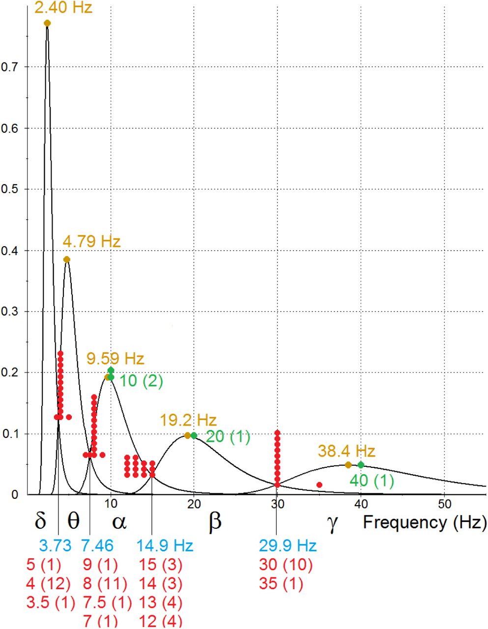
The graphs are the estimated PDFs of the frequencies of a three-neuron ring oscillator and four cascaded toggles. All of the PDFs were determined by the estimated mean and variance of neuron delay times. The five intervals defined by the intersections of consecutive PDFs are labeled with Greek letters to distinguish them from EEG frequency bands, which are often written in the Roman alphabet. The intersections and modes are labeled in blue and yellow, respectively. Also shown in red and green are frequencies that are commonly cited as partition points separating the EEG frequency bands and peak frequencies of three of the bands. Numbers in parentheses and numbers of data points show how many times each frequency was cited.
5.5. Synchronization
The EEG frequency bands and associated behavioral and mental states are consistent with the advantages of synchronous logic systems.
5.5.1. Synchronous logic systems
Logic systems have a timing problem in ensuring the various subcircuits change states in the correct chronological sequence. Synchronous logic systems generally have simpler circuit architecture and fewer errors than asynchronous systems. This is the reason nearly all electronic logic systems are synchronized by an enabling pulse to each component circuit, so that whenever any components change states, they change simultaneously. The enabling pulse in such systems is usually produced by an oscillator. The enabling input in Fig 2E and the oscillators in Fig 3 illustrate how such synchronization is possible with neural networks.
Timing problems are greater in sequential logic than in combinational logic, and greater in parallel processing than in serial processing. Much of the information processing in the brain involves sequential logic and nearly all of it is parallel. The selective pressure for synchronization in the brain would have been high, and the neural implementation proposed here is quite simple.
The processing speed in a synchronous system depends largely on the enabling oscillator’s speed. A large system like the brain that performs many diverse functions may have several different processing speed requirements. The trade-off for greater processing speed is a higher error rate. Functions that can tolerate a few errors, and that need fast results with many simultaneous small computations, require high processing speeds. Functions that are less dependent on speed or massive computation, or that require few errors, or whose component networks are large and complex and therefore slow to change state, call for slower processing.
5.5.2. Synchronization and EEG frequency bands
The EEG frequency bands and associated behavioral and mental states are consistent with the function of multiple frequencies that was suggested in the preceding paragraph. Gamma waves (high frequencies) are associated with vision [43, 44] and hearing [Mably 14], which make sense out of massive data input in a few milliseconds. Beta waves are associated with purposeful mental effort [20], which may involve less data input while requiring few errors and complex operations. Alpha waves are associated with relaxed wakefulness [20], theta waves with working memory and drowsiness [20, 45], and delta waves with drowsiness and sleep [20]. These categories require successively slower information processing, and they have corresponding EEG bands of lower frequencies.
Cascaded oscillators can produce this neural activity. A neural oscillator can synchronize state changes in neural structures by enabling them simultaneously. The enabling oscillator pulse by itself does not produce any state changes. It only forces states to change simultaneously when they do change. So the initial ring oscillator’s high frequency signal could simply be connected directly and permanently to the enabling gates (as illustrated in Fig 2E) of networks in the visual and auditory cortexes, the first toggle’s signal to networks in the prefrontal cortex for purposeful mental effort, etc. A large number of neural structures synchronized in this way by cascaded oscillators would exhibit the bands of matched periods found in EEGs.
6. Results and explanations of known phenomena
6.1. Short-term memory controversy
Cascaded oscillators and NFFs suggest a resolution to the question of whether short-term memory depends on neurons firing persistently or in brief, coordinated bursts [7, 8]: Memory is stored by persistent firing in flip-flops [4], and the coordinated bursts observed along with the persistent firing are due to the stored information being processed by several neural structures whose state changes are synchronized by a neural oscillator. An example of such short-term memory processing is a telephone number being reviewed in a phonological loop.
6.2. Electroencephalography
6.2.1. EEG frequency bands’ peaks and boundaries
Fig 5 shows that the cascaded oscillators hypothesis is supported by the available data for neuron delay times and EEG frequency band peaks and boundaries. The graphs in Fig 5 are the estimated oscillator PDFs derived from a description of the range of neuron delay times. The cascaded oscillators hypothesis implies that the EEG frequency band boundaries are the intersections of consecutive oscillator frequency PDFs. The graphs show the intersections of the estimated oscillator PDFs (in blue) are within the ranges of estimated EEG frequency band boundaries (red). The hypothesis also implies the EEG band peaks are the same as the oscillator PDF peaks. Fig 5 shows the available estimates of three EEG band peaks (green) are close to the peaks of the estimated oscillator PDFs (yellow).
These close fits also show that the available data support the main implication of the cascaded oscillators hypothesis (that the EEG bands have the same distributions of frequencies as the cascaded oscillators) and the implication that the ratios of peaks and boundaries of the major EEG bands are powers of two.
6.2.2. EEG phenomena
The cascaded oscillators hypothesis answers the EEG questions raised in the section on unexplained phenomena.
What produces the widespread, synchronized, periodic firing? The firing is periodic because neural structures are being enabled by an oscillator. The periodic firing is widespread because many neural structures are being enabled. The firing is synchronized because the neural structures are being enabled by the same oscillator.
What is the function of this widespread synchronization? The function of synchronization is timing error avoidance in processing information.
What produces and what is the function of the wide distribution of EEG frequencies in bands? The frequencies occur in bands because the frequencies are produced by different oscillators. The wide distribution of frequencies is due to the octave relationship between cascaded oscillators (100% exponential growth in periods with each successive oscillator by equation 4) and several oscillators. The distribution of frequencies within each band is due to the variance of neuron delay times in the initial oscillators in the cascades (equations 5). The function of the wide distribution of frequencies is meeting the needs of different brain functions in the trade-off between speed and accuracy.
What produces the unimodal distribution in each band and the octave relationships between the peaks and boundaries? The unimodal distributions are due to the normal distribution of neuron delay times in the initial ring oscillators in cascades of oscillators. This makes the distribution of periods of each oscillator normal and the distributions of frequencies unimodal. The ratio of consecutive boundaries and peak locations is 2 because consecutive cascaded oscillators increase the oscillation period by a factor of 2 (equations 4, 8, 9).
What determines the specific frequencies of the peaks and boundaries? The number of neurons in the ring oscillators must be the minimum of 3 to produce the high frequencies in the gamma band. Equations 8 and 9 show the EEG band boundaries and peaks are determined by this number (n = 3), the ring oscillators’ delay parameters μd and σd, and the boundary or peak number i.
Why do gamma oscillations peak at about 40 Hz? The three-neuron ring oscillator is the fastest neural ring oscillator. The estimated peak frequency from equation 9 is 38.4 Hz (illustrated in Fig 5).
Why does the gamma band contain frequencies that are considerably faster than 40 Hz? The frequencies vary because of the variance in neuron delay times in the initial oscillators. As Fig 5 illustrates, all of the oscillator frequency distributions are skewed to the right, with the initial oscillator producing frequencies substantially greater than 40 Hz. In the particular estimate of Fig 5, 2% of the frequencies are greater than 75 Hz, and 0.4% are greater than 100 Hz.
Why is there little agreement on the boundaries separating the EEG bands? The oscillators hypothesis implies that the estimates of EEG band boundaries are estimates of the intersections of the oscillators’ PDFs. This makes estimating boundaries difficult for two reasons.
The oscillators hypothesis implies that the probability of an EEG frequency being observed has a local minimum near each intersection of consecutive oscillator PDFs. This means that in a random sample of observed EEG frequencies, relatively few will be near the intersections. A small number of data points has a negative effect on the accuracy of estimates.
The overlapping oscillator PDFs (Fig 5) imply the distributions of EEG frequencies associated with the various behavioral and mental states have overlapping ranges rather than discrete bands. Because two PDFs are equal at their intersection, a frequency near the intersection of two PDFs is almost equally likely to be produced by either of two oscillators. That is, an observed EEG frequency near a band “boundary” is almost equally likely to be observed along with the behavioral and mental state that defines the band on either side of the intersection. This makes obtaining accurate estimates of band “boundaries” especially difficult.
7. Testable predictions
7.1. Constructed neural networks
Any of the networks in the figures could be constructed with actual neurons and tested for the predicted behavior. Constructing and testing NFFs was discussed in [4]. The ring oscillator of Fig 3 may be simple to construct and test. The predicted behavior is oscillating outputs for all three neurons with a period that is twice the sum of the neurons’ delay times, and phases uniformly distributed over one cycle.
7.2. A statistical test of the cascaded oscillators hypothesis
7.2.1. The data problem
Although the hypothesis that cascaded oscillators produce EEG phenomena is consistent with available data, as illustrated in Fig 5, the data are too imprecise for a rigorous statistical test of the hypothesis. The estimates found here for the neuron delay time parameters μd and σd were based on a rough description of the range of synapse delay times. Available estimates of the EEG frequency bands’ peak frequencies are few, estimates of band boundaries vary widely, and both types of estimates are routinely rounded to whole numbers. Some researchers do not attempt to estimate a boundary between bands, instead giving a whole number as the upper endpoint of one band and the next consecutive whole number as the lower endpoint of the next band. Estimates of means and variances of both neuron delay times and EEG frequency bands are apparently nonexistent.
7.2.2. A simple test of the cascaded oscillators hypothesis from sampling data
A simple, rigorous test of the cascaded oscillators hypothesis is possible. As stated in the introduction, all predicted EEG phenomena follow from the main implication that the EEG bands and cascaded oscillators have the same distributions of frequencies. This implication can be tested statistically with random samples and the distribution relations of equations 5. As discussed previously, neuron delay times should be approximately normally distributed by the central limit theorem. This implies cascaded oscillator periods are also approximately normally distributed. A normal distribution is completely determined by its mean and variance. So it remains to be shown that EEG band periods are normally distributed, and that EEG band periods and oscillator periods have equal means and variances.
The neuron delay time parameters μd and σd can be estimated from a random sample of neuron delay times. These estimates can be used to estimate the oscillator period distribution parameters μi and σi from equations 5. The mean and variance of the periods of one or more EEG bands can be estimated from a random sample of EEG periods (or frequencies). With standard tests for equal means and variances, the EEG estimates can be compared to the oscillator estimates of μi and σi. The EEG sampling data can also be used to test EEG band periods for normal distributions. If the application of the central limit theorem to neuron delay times may be questionable, neuron delay times can also be tested for a normal distribution with the neuron delay time sampling data.
7.2.3. Caveats
Because the oscillators’ frequency ranges overlap (Fig 5), the band to which an observed EEG period or frequency is assigned should be determined by the observed behavioral and mental state that defines a band, not by predetermined endpoints of bands. If EEG sampling data are measured in frequencies, they must be converted to periods before computing the sample mean and variance. (The period of the sample mean of frequencies is not the same as the sample mean of periods.) Sampling data should not be rounded to whole numbers. In using equations 5 to find the estimated oscillator parameters, recall that the value of n must be the minimum of 3. Sampling data for neuron delay times and EEG periods (or frequencies), or even estimates of means and variances, may already be available in some database.
Although it is possible that EEG frequencies are produced by cascaded oscillators with initial oscillators that are made up of specialized neurons whose delay times are different from the general population of neurons, this appears to be unlikely. Fig 5 shows the EEG frequency distributions are at least close to the values predicted by the general description of the range of neuron delay times that was used here to estimate oscillator neuron delay time parameters.
Moreover, neurons in general and initial oscillator neurons in particular may have both evolved under selective pressure to function as fast as possible.
8. Acknowledgements
The simulation was done with MS Excel. Network diagrams were created with CircuitLab and MS Paint. Graphs were created with MS Excel, Converge 10.0, and MS Paint. The author would like to thank Arturo Tozzi, David Garmire, Paul Higashi, Anna Yoder Higashi, Sheila Yoder, and especially Ernest Greene and David Burress for their support and many helpful comments.


