

Abstract
The development of crops with deeper roots holds substantial promise to mitigate the consequences of climate change. Deeper roots are an essential factor to improve water uptake as a way to enhance crop resilience to drought, to increase nitrogen capture to reduce fertilizer inputs and to increase carbon sequestration from the atmosphere to improve soil organic fertility. A major obstacle to achieving these improvements is the bottleneck in the high-throughput phenotyping of field-grown roots. We address this bottleneck with DIRT/3D, a newly developed image-based 3D root phenotyping platform, which measures 16 architecture traits in mature maize root systems. DIRT/3D computed reliably all 16 traits on a test panel of 12 contrasting maize genotypes. The analysis of the maize panel validated traits such as distance between whorls, and the number, angle, and diameters of crown and brace roots. Overall, we observed a coefficient of determination of r2>0.84 and a high broad-sense heritability of  for all traits. Means of the 16 traits and a newly developed descriptor to characterize a complete root architecture distinguished all genotypes. DIRT/3D is a step towards automated quantification of highly occluded maize root systems in the field and will support breeders and root biologists to improved carbon sequestration and food security in the face of the adverse effects of climate change.
Introduction
Evaluating the information encoded in the shape of a plant as a response to environments is essential to understand the function of plant organs (Bucksch 2011). In particular, roots exhibit shape diversity that is measurable as variation in rooting angles, numbers of roots per type, length, or diameter of roots within a root system (Lynch and Brown 2012). An understanding of variation in root systems facilitates breeding for favorable root characteristics to improve yield in suboptimal conditions, including those resulting from climate change (Lynch 2013). Improving root phenotypes through crop breeding and management holds promise for improved food security in developing nations, where drought, low soil fertility and biotic constraints to root function are primary causes of low yields, and also for reducing the environmental impacts of intensive agriculture by reducing the need for intensive fertilization and irrigation (Lynch 2019). Root traits also offer opportunities to improve C sequestration (Paustian, Lehmann et al. 2016). These challenges demand efforts across a range of disciplines, from mathematics over computer science to plant biology and applied fields like plant breeding and agronomy (Bucksch, Atta-Boateng et al. 2017, Bucksch, Das et al. 2017).
A major interdisciplinary challenge in root biology is the development of deeper rooting crop varieties. Deeper roots promise a three-fold impact: they improve drought resilience, lower fertilizer input, and decrease atmospheric carbon. Deeper roots improve drought resilience to stronger and more frequently occurring droughts (Ault 2020) by tapping into water in deep soil domains (Lynch and Wojciechowski 2015). Nitrogen capture increases when roots grow deeper because nitrogen diffuses into and accumulates in deeper soil layers (Lynch 2019). Deeper rooting crops increase carbon sequestration (Smith, Martino et al. 2007) mostly by depositing more organic residues in soils, thereby replenishing carbon after harvest (Paustian, Agren et al. 1997). An important tool in breeding deeper roots is the large-scale automated evaluation of root traits in the highly occluded root system architecture (Topp, Bray et al. 2016). Maize (Zea mays) in particular, with over 700 Mt of maize production world-wide (Ranum, Peña-Rosas et al. 2014), is a prime target for improving rooting depth. However, measuring important root traits for deeper rooting in maize is hampered by the availability of advanced root phenotyping methods on the field-scale (Kuijken, van Eeuwijk et al. 2015). Therefore, the research community has pushed for the development of a root phenotyping system that operates under field conditions (Paez-Garcia, Motes et al. 2015).
The field vs. lab complement
The majority of existing phenotyping methods to evaluate root architecture non-destructively emerged from laboratory settings. These methods range from fully automatic (Galkovskyi, Mileyko et al. 2012) to manually assisted (Lobet, Pagès et al. 2011) and consider a variety of growth systems like gel cylinders (Iyer-Pascuzzi, Symonova et al. 2010), rhizotrons (Nagel, Putz et al. 2012, Rellán-Álvarez, Lobet et al. 2015), mesocosms (Nagel, Putz et al. 2012) and germination paper (Falk, Jubery et al. 2020). Root phenotyping under lab conditions necessitates the use of constrained growth containers (Poorter, Bühler et al. 2012, Bourgault, James et al. 2017), artificial growth media (Oliva and Dunand 2007), and environments that potentially alter root system architecture (de Dorlodot, Bertin et al. 2005, Draye, Thaon et al. 2018). Therefore, it is essential to translate phenotyping experiments from the lab into repeatable field experiments (Zhu, Ingram et al. 2011, Bucksch, Burridge et al. 2014, Poorter, Fiorani et al. 2016).
In contrast, root phenotyping in the field is currently either invasive or destructive. Invasive procedures record small sections of the root with minirhizotron cameras placed in the soil (Gray, Strellner et al. 2013, Yu, Zare et al. 2019). Still, these procedures are incapable of recording the full root system. Therefore, investigating root system architecture relies heavily on the destructive excavation of the root crown. Shovelomics is the standard field-ready protocol to excavate root systems in the field (Trachsel, Kaeppler et al. 2011). It was initially developed for maize and undergoes a constant refinement by the root research community (Zheng, Hey et al. 2020). Other crops, including common bean (Phaseolus vulgaris) and cowpea (Vigna unguiculata) (Burridge, Jochua et al. 2016), wheat (T. aestivum) (Slack, York et al. 2018, York, Slack et al. 2018), rapeseed (Brassica napus) (Arifuzzaman, Oladzadabbasabadi et al. 2019) and cassava (Manihot esculenta) (Kengkanna, Jakaew et al. 2019) have specialized shovelomics protocols in place. However, the manual excavation of the crown root system, followed by visual scoring and manual trait measurement, is difficult and subjective to the researcher.
Digital imaging of root traits in 2D
In response, software to measure root traits in simple digital images became available. Approaches to record root traits in the field use different methods in terms of software platforms and imaging setups. The largest software platform is DIRT (Das, Schneider et al. 2015), which provides online image processing for over 650 users following an easy to reproduce imaging protocol. For imaging, DIRT needs a tripod, a consumer camera, and a black background with a white circle. Just recently, DIRT enabled projects associated with root architecture and micronutrient content (Busener, Kengkanna et al. 2020), discovered unknown gene functions (Bray and Topp 2018) and translated traits from the lab to the field (Salungyu, Kengkanna et al. 2020). More sophisticated and expensive imaging setups use specialized tents (Colombi, Kirchgessner et al. 2015) and carefully designed imaging boxes (Grift, Novais et al. 2011, Seethepalli, Guo et al. 2019), along with computationally cheap traits, for use on personal computers. The user can, therefore, choose a system that suits the project needs. Systems generally vary in the number of instruments, tools, and samples transported between the lab and field site, as well as the cost of the imaging setup and hardware requirements. However, all these systems share a single obstacle: Resolving the highly occluded branches of a dense 3D root system. The occlusion challenge arises when the 2D image projection of the 3D branching structure ‘hides’ information of branching locations. Hence, the branching information is unrecoverable and lost.
Digital imaging of root traits in 3D
3D approaches are capable of resolving even highly occluded branching structures (Bucksch 2014). Gel systems were among the first methods to measure fully resolved 3D root systems of younger roots (Clark, MacCurdy et al. 2011, Topp, Iyer-Pascuzzi et al. 2013) and to capture some of their growth dynamics (Symonova, Topp et al. 2015). The bottleneck of imaging and measuring older root systems in constrained growth containers filled with soil, however, remained. Therefore, X-Ray computed tomography (CT) became a widely used tool to phenotype roots in pots filled with soil and soil-like substrates (Pfeifer, Kirchgessner et al. 2015). These lab developments revealed for example new characteristics in maize root development (Jiang, Floro et al. 2019). The X-ray CT approach is, in its applications, comparable to magnetic resonance imaging (MRI) (Metzner, Eggert et al. 2015). MRI also provides a 3D model of the root (van Dusschoten, Metzner et al. 2016) and can be used for time-lapse imaging of growth processes (Jahnke, Menzel et al. 2009). The benefits of both X-Ray CT and MRI are substantial and subject to scientific discussion (Fischer, Lasser et al. 2016). However, both technologies do not meet the needs for large-scale field studies: Firstly, both technologies restrict plant growth to the size of a given growth container. The restriction to smaller sizes is proportional to higher achievable resolution. Therefore, it is common to observe an immature “pot phenotype” instead of a relevant phenotype grown in field soils (Poorter, Bühler et al. 2012, Bourgault, James et al. 2017). Secondly, both methods are relatively slow and typically take 30 minutes or more to collect root imaging data. Extremes of several days are reported for X-Ray CT systems to achieve the resolution of root hairs (Keyes, Daly et al. 2013, Sozzani, Busch et al. 2014). An additional constraint is the cost of constructing, operating, and staffing such facilities, few of which are devoted to root studies.
In response to these phenotyping limitations, we developed DIRT/3D as an automatic 3D root phenotyping system for excavated root systems grown in agricultural fields. Our approach consists of a newly developed 3D root scanner and root analysis software. The 3D root scanner captures image data of one excavated maize root in about 5 minutes. Our software uses the image data to produce a colored 3D point cloud model and to compute 16 root traits. The computed traits measure individual roots and also characterize the complete root system. Individual root traits include number, angle, and diameters of crown and brace roots. Traits like eccentricity or the distance between brace and crown root whorls characterize the root system. We also introduce a new 3D whole root descriptor that encodes the arrangement of roots within the root system.
Results
DIRT/3D enables automatic measurement of 3D root traits for field-grown maize
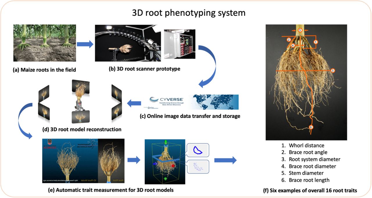
We developed DIRT/3D (Digital Imaging of Root Traits in 3D) system to phenotype excavated root crowns of maize (Figure 1). The system includes a 3D root scanner and a suite of parameter-free software that reconstructs field-grown maize roots as a 3D point cloud model. The software also contains algorithms to compute 16 root traits.

The 3D root scanner (b) fits roots grown in the field (a) and excavated with the Shovelomics protocol (Trachsel, Kaeppler et al. 2011). The scanner, with ten synchronized industrial cameras mounted on a curved frame, acquires about 2000 images of the root. The images are transferred to and stored in the Cyverse Data Store (Merchant, Lyons et al. 2016) (c). The 3D reconstruction is computed with DIRT/3D’s structure-from-motion software (d) and yields the resulting 3D root model (e). Overall, the analysis software calculates 16 root traits from the 3D point cloud of the root system. The image in (f) shows examples for the trait classes angle, diameter, and length. All developed software methods are open source and executable as a Singularity container (Kurtzer, Sochat et al. 2017) on high-performance-computing systems.
The 3D root scanner (Figure 2) utilizes ten industrial cameras mounted on a rotating curved frame (Figure 2a) to capture images from all sides of the maize root (Supplementary Material 1). Scanning of one maize root completes in five minutes. After obtaining the image data, we reconstruct a 3D point cloud of the root system (Figure 3A). By analyzing thin level sets of the 3D point cloud, DIRT/3D revealed traits behind multiple layers of occlusions (Detailed pipeline in Supplementary Material 2). For example, DIRT/3D measures the distance between the brace and crown root whorl and the number of brace and crown roots. DIRT/3D also tracks every individual root within the root system, starting from the stem down to the emerging lateral in the excavated root crown. Each individually tracked root enables the measurement of numbers, angles, and diameters at the individual root level (Figure 1f).

(a) 3D root scanner captures images of an excavated maize root grown under field conditions. (b) The stepper motor rotates the curved metal frame with the mounted cameras around the root. (c) The fixture keeps the root in place during scanning. (d) The adjustable camera shelves allow for the free positioning of each camera. The CAD drawings of the 3D root scanner are available in Supplemental Material 3.


A. The 3D reconstruction of the maize root architecture using 2000 images (including side view from the bottom, side view from the top, front view, bottom view, and top view). The resolution of each image is 3872 pixels × 2764 pixels. The resulting point cloud contains 439.918 points (Supplementary Material 4). B. Comparison between excavated maize root systems and their 3D models: Examples of excavated maize root crowns and their 3D models from a test panel of 12 genotypes. We captured 2D images of the original root sample for each genotype. We built corresponding 3D root models (ply point cloud format) from 2D image data using our automatic parameter-free algorithms. Visual comparison of the 2D views of real roots and their respective 3D root models shows that root architecture, along with the color, is reconstructed (Supplementary Material 5). All 3D models used in the paper are available as .ply file in Supplementary Material 18.
We used a panel of 12 maize genotypes with 5-10 replicates per genotype to validate the DIRT/3D pipeline. For our validation trial, the 3D root scanner captured images at pan intervals of 1 degree and tilt intervals of 10 degrees. Figure 3B shows a visual comparison of the captured root architectural variation between the genotypes.
Level set scanning enables extraction of traits from 3D root models
We developed a new method to perform a top-down level set scan of the 3D root model to compute 3D root traits. For a vertically aligned model, we slice the 3D root model from top to bottom at consecutive depth levels (Figure 4). The imaging volume of the scanner is constant, and therefore the number of slices per root is variable. Two benefits result from the fixed scanning volume. First, the transformation to mm is constant, and second, the optimal slice thickness can be determined experimentally for all roots. Therefore, all parameters are constants in the algorithm. Here, a level set image is the vertical 2D projection of each slice onto a plane (Cochard, Delzon et al. 2015, Dinas, Nikaki et al. 2015, Hyun, Bae et al. 2016) representing the sequential distribution of roots into deeper soil levels (Figure 4 (b)-(e)).
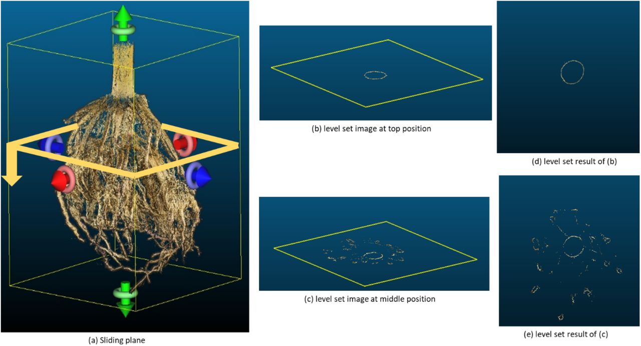
(a) A sliding plane scans the 3D root model from top to bottom to acquire a level set image sequence. The information content per level set image varies with depth and generally encodes the points at a pre-defined distance to the sliding plane. For example, at the top (b and d), only information about the stem appears in the level set image. At a middle position (c and e), individual roots are visible as additional circles.
Ideally, each root is a closed circle in the level set plane. However, roots are under-sampled or affected by noise such that the contours of some roots are disconnected. A video sequence of all level set images would result in a flickering effect. Therefore, we use a phase-based frame interpolation technique (Meyer, Wang et al. 2015) to smooth the level set image sequence. This method estimates transition frames between the level set images, which is equal to an up-sampling process of the 3D point cloud (Waki 2016). Insufficient sampled locations of the root models are interpolated, which results in a smooth connection of formerly disconnected contours on level set images (Zhao, He et al. 2018). A comparison of the original and smoothened sequence of level set images shows the increased density of the 3D root model (Supplementary Material 6).
The active contour snake model identifies individual roots per level set image
The image sequence of the smoothened level sets is the key to compute the location and size parameters of individual roots. Applying the active contour snake model (Kass, Witkin et al. 1988) to each level set image results in a curve that circumscribes each individual root in the level set image (Mugerwa, Rey et al. 2019). Each curve contracts and moves towards the closed boundaries of an individual root by minimizing a partial differential equation, where image boundaries represent a low energy state for the active contour. The partial differential equations formulize a trade-off between an internal and external energy term. The internal energy describes the continuity and smoothness of the contour to controls for curve deformations, and an external energy that describes how well the contour fits the individual root (Zhao, He et al. 2018).
Our algorithm initializes a circle around each individual root in each level set as an initial input to the minimization of the active contour snake (Supplementary Material 8). During the iterative minimization of the energy function, we use a periodic boundary condition to enforce a closed curve. The resulting closed boundary curves represent first estimates of individual roots and used as input to compute a binary mask for each level set image sequence using Otsu’s binarization method (Moghaddam and Cheriet 2012). We adopt the connected components labeling method to distinguish and label each closed-boundary object, representing individual roots (Playne and Hawick 2018). The result of connected components labeling is a multiple segmentation of individual roots represented by colored components (Figure 5).

(a) shows five sample images from the smoothened level set images. (b) shows the corresponding results from the active contour snake method. Each extracted individual root is color-coded with connected component labeling. The active contour snake model detects individual roots in each level set image. A video showing the active contour snake evolving process is available in Supplementary Material 7.
However, due to the complexity of the maize root system, roots intertangle or adhere to each other. In an image of the level set sequence, the entanglement will be visible as one connected component instead of two distinct components. We use the watershed segmentation to segment the overlapping root (Supplementary Material 9). The idea behind the watershed algorithm is to interpret grey values in the image as a local topography or elevation. The algorithm uses pre-computed local minima to flood basins around them. The algorithm terminates the flooding of a basin when the watershed lines of two basins meet. The Euclidean Distance Transform (EDT) of the image allows for direct detection of the local minima (Fabbri, Costa et al. 2008). In that way, watersheds assign each pixel to a unique component and allows the distinction entangled roots per level set image (Roshanian, Yazdani et al. 2016).
A combination of Kalman filters and the Hungarian algorithm tracks individual roots
We developed an individual root tracking method by adopting a combination of Kalman filters and the Hungarian algorithm (Sahbani and Adiprawita 2016). The algorithm detects individual roots for consecutive level set images. Once individual roots are detected, the Hungarian algorithm matches the corresponding individual roots across the level set images. To improve the speed of the Hungarian algorithm, we use a Kalman filter to predict matching individual roots in consecutive level set images (Figure 6). Behind the scenes, the tracking algorithm builds a mathematical model of expected depth development of the root. In doing so, the algorithm uses the current position, relative speed, and acceleration of individual roots to predict their location in the following level set image.
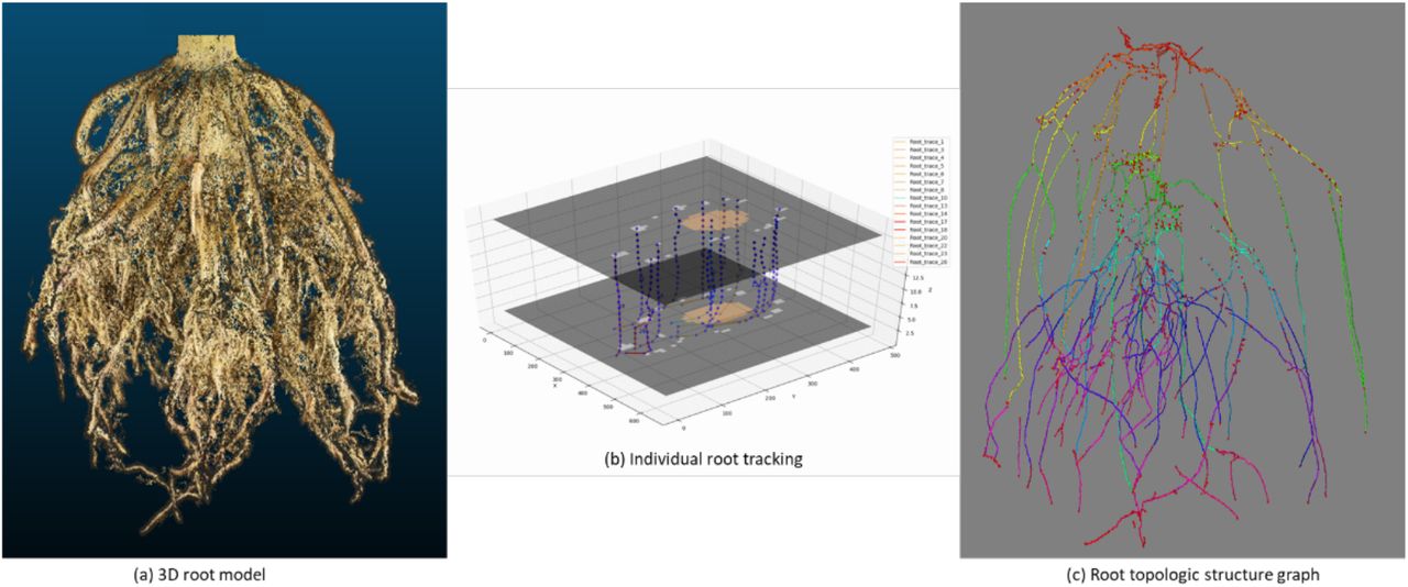
(a) 3D model of a field-grown maize root generated by the DIRT/3D reconstruction. (b) Visualization of the tracking process of individual roots from level set images. Two level set images are visualized with 50% transparency to show the tracking of individual roots in 3D space. (c) 3D visualization of the root topologic structure graph consisting of all tracked trajectories. The structure graph encodes the arrangement of roots within the roots system as a data structure to compute on. The graph data structure includes the detected whorls and the connected brace and crown roots. Each individual root was color-coded by nodes and depth values.
During the sequential processing of all level set images, we calculate the diameters of the minimal bounding circle that covers all points in all level set images in a 2D projection. Table 1 lists all 16 root architecture traits that DIRT/3D computes.
Description of DIRT/3D traits. Traits describe either a root system (RS) characteristic or measure an individual root (IR) within the root system.
3D root traits correlate at individual root and root system level
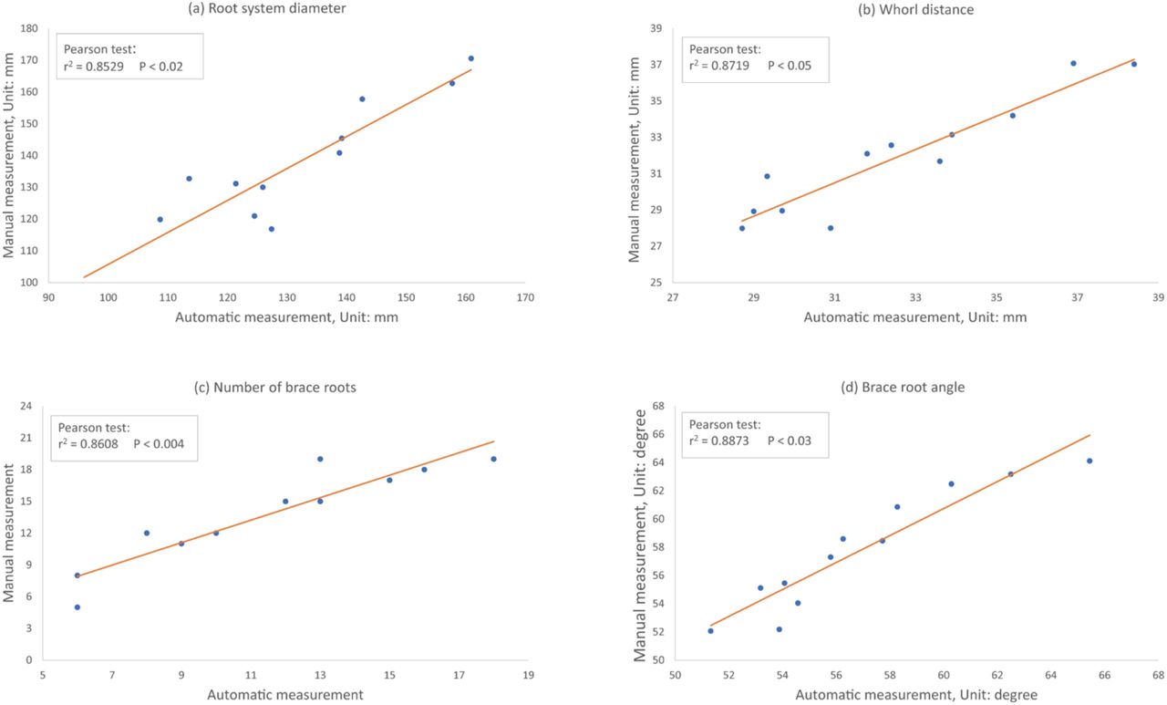
To test the accuracy and precision of DIRT/3D, we correlated the trait values measured automatically in the 3D point clouds and manually on the root crown. We validated manually measurable traits such as root system diameter, whorl distance, number of brace roots, and brace root angle. Computing the validated traits executes all coded lines of our software and covers all possible combinations of functions. Therefore, we consider the software to be validated in its calculations for other traits if the code is not changed. The correlation analysis of the each of the chosen validation traits showed r2>0.85 and p < 0.05 for the Pearson test (Figure 7 a-e).

Each point is the average trait value of 5-10 replicates of one of the 12 genotypes of our test panel. Pearson tests evaluated the root traits (a) the diameter of the whole root system, (b) whorl distance, defined as the distance between the brace root and crown root whorl closest to the soil line, (c) the number of brace roots, (d) brace root angle and (e) brace root diameter.
Broad sense heritability suggests high repeatability of the observed root trait values
Broad-sense heritability,  for all traits (Figure 8) is computed as the ratio of total genetic variance to total phenotypic variance (Falconer 1989) to demonstrate the repeatability of the initial fields trial. For quantitative plant traits, the broad-sense heritability across multiple varieties eliminates the time-consuming steps of hybridization and population development for determining
  . We observed a broad-sense heritability
  for all traits except brace root angle, which indicates a moderately strong genetic basis of the computed traits. Seven of the computed traits resulted in
  (Figure 8), which indicates that the calculated traits show minimal variation within genotypes.

Phenotypes vary between the individuals because of both environmental factors, the genes that control traits, as well as various interactions between genes and environmental factors. We computed broad-sense heritability for all 3D traits in Table 1. All but one trait suggests a strong genetic basis to explain the observed inter-genotypic variation with  .
.
3D root traits distinguish genotypes in the test panel
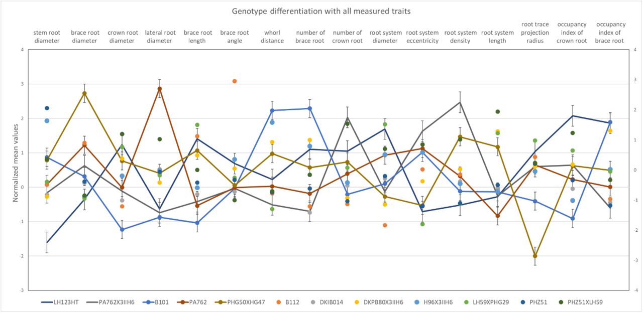
The 16 computed 3D root traits distinguished genotypes by their means (Figure 9). Overall, we found that no single trait classifies all genotypes. However, an ANOVA test revealed that the means of each pair of genotypes distinguishes in at least four traits (Supplementary Material 17). For example, genotype PA762 and B101 show a significant difference with traits such as brace root diameter and lateral root diameter. However, B101, PA762, and PHG50XHG47 do not show separable mean values in the brace root angle.

We normalized all the mean trait values of computed 3D root traits from DRIT/3D. Colored points denote the normalized mean values of the 16 root traits. The lines guide the reader visually to explore the phenotypic variation between genotypes of the test panel. For example, the mean of genotype PA762 and B101 distinguishes in brace root diameter and lateral root diameter; Genotype PHG50XHG47 and PA762 distinguish in the root projection radius. However, B101, PA762, and PHG50XHG47 do not show distinguishing mean values in the brace root angle.
Whole root descriptor distinguishes the unique spatial arrangement of individual roots for all genotypes
We introduce a 3D variation of the established D-curve for 2D images (Bucksch, Burridge et al. 2014) as a whole root descriptor. We compute the descriptor from the sequence of level set images derived from the reconstructed 3D root models. For each level set image, we compute the number of pixels that represent roots as a measure for the area. We found that the accumulation of root area across the level-set images is an intrinsic characteristic of each genotype (Supplementary Material 10). The descriptor is robust to outliers and measurement errors because it relies on the cumulative distribution function (Chun, Han et al. 2000, Lee 2001, Kyurkchiev 2015). Figure 9 shows the results of the test panel of the 12 genotypes used the maize test panel. The whole root descriptor distinguished the unique arrangement of individual roots for all 12 genotypes as a characteristic mean curve, as shown in Figure 10.

The descriptor encodes the spatial arrangement of individual roots within the root system as a function of the excavation depth. We define the curve of the cumulative root system area as the cumulative distribution function (CDF) of the area per level set for each genotype. The error bar denotes the standard error of the normalized root area. Each genotype associates with a characteristic CDF curve (colored coded). All genotypes distinguish visually from each other in their curve characteristics.
Discussion
The presented 3D system to measure traits in highly occluded root systems is a significant advance in root phenotyping because it measures highly occluded traits such as whorl distance and number or brace and crown roots in the dense maize root system. Furthermore, the presented methods push against the frontier of phenomics by presenting a whole root descriptor for plant root architecture. For the test panel of twelve genotypes, a minimum of four traits distinguished all genotypes. In contrast, the whole root descriptor is one characteristic that distinguished all genotypes with one mathematical expression. Both together, put forward the unaccomplished goal of phenomics to measure the comprehensive appearance of a continuously reshaping phenotype (Houle, Govindaraju et al. 2010).
However, some algorithmic and technical challenges remain to exploit the utility of 3D root phenotyping for breeders fully. To date, standard calibration procedures for structure from motion scanners with multiple cameras are rare (Conte, Girelli et al. 2018). Further research will focus on the details of the photogrammetric calibration of the 3D root scanner, which will allow for thinner cross-section slices during level set extraction. We believe that root models of higher resolution will enable the reconstruction of a more detailed root architecture to obtain measures of all nodes in the maize root system.
We demonstrated the possibility to retrieve high geometric detail from field excavated roots. We even argue that it will be possible to obtain geometrically complete measurements in the sense of Euclid’s definitions in Elements I-IV and VI (Casey 2015). Local measurements of length, diameter, and angle are sufficient to reconstruct every solid 3D object if sampled at sufficiently high rates. Again, research on the calibration technique used for structure from motion scanners seems likely to be the limiting factor in achieving the needed resolution. Assembling the complete geometrical system of the root system will allow us to describe the whole root system and its spatial arrangements in one single mathematical construct. We presented a first 3D whole root descriptor that is similar to the validated D- and DS-curve for 2D images (Bucksch, Burridge et al. 2014). We encoded root architecture as an aggregate of the extracted 3D traits and could reliably distinguish the roots of different genotypes for a small diversity panel. However, our approach neglects root density and root order, which limits the encoded detail. An extension of the presented whole root descriptor would enable the quantification of morphological differences within homozygous populations to understand the variation of architecture arrangements. Besides, the comparison between plant species with similar topological organization but different geometric growth such as dense first order laterals yet with varying patterns of curvature along the root, would be enabled.
The observed broad-sense heritability suggests a strong repeatability of our first study ( for most traits). Repeatability, paired with near geometric completeness, indicates the presence of a local and global architecture control by genes. Local control relates to phenes that assemble the architectural phenome of roots as a set of mappable and locally measurable traits (Lynch and Brown 2012). However, it is still an open question if a “global control phene” of root architecture phenes exists (Jiang, Floro et al. 2019) unless we can map whole root architectures that are geometrically complete. A necessary step towards answering this question from a mathematical point of view is to define a mathematical basis of locally controlled traits or phenes. Since phenes are often mappable to genes (Yablokov 1986), a mathematically independent basis formed by phenes would open ways for the alternative hypothesis that roots have access to a spectrum of architectures that acclimatize to their micro- and macro-environments via their species-specific phenes.
Conclusion
Our 3D phenotyping system is arguably the first optical system to handle highly occluded and mature root systems in the field. It is worth noting that the time required to collect the imaging data is around five minutes, which is significantly less than a typical X-Ray scan at a comparable resolution (Paya, Silverberg et al. 2015). Unlike many root phenotyping methods developed under lab conditions, our system measures maize roots grown under field conditions. We also demonstrated that our system reliably computes previously inaccessible traits, such as whorl distance, and the number and angles of both brace and crown roots. We validated our system for the root trait classes of number, angle, diameter, and length. Validation results demonstrate the reliability of our system with correlations of r2 > 0.84 for most traits and P-values < 0.005. From our analysis, we concluded that DIRT/3D could extract 3D root traits accurately at the individual and system levels.
Our open-source software is available to the whole plant science community on GitHub, and can be deployed within a platform-agnostic Singularity container to be executed independently of the operating system (Supplementary Material 11) (https://github.com/Computational-Plant-Science). The use of Singularity containers will allow for integration with cyber-infrastructures such as CyVerse. These containers can run on any high-performance computing system that has the Singularity environment installed.
The only user interaction in our system is to place the root in the scanner, which could be replaced by a robot. Hence, we see our system as the first milestone towards automated root trait measurements in the field. Our belief stems from ongoing developments in agricultural robotics that will excavate field roots “on-the-go” (Shi, Choi et al. 2019) in the foreseeable future. In that way, our system supports breeders and root biologists in the development of crops with increased water uptake, more efficient nitrogen capture and improved sequestration of atmospheric carbon to mitigate the adverse effects of climate change without compromising on yield gains.
Material and Methods
Plant material
Plants were grown at The Pennsylvania State University’s Russell E. Larson Agricultural Research Center (40° 42’40.915” N, 77°, 57’11.120’’W) which has a Hagerstown silt loam soil (fine, mixed, semi-active, mesic Typic Hapludalf). Fields received fertilization with 190 kg nitrogen ha−1 applied as urea (46-0-0). The sites had drip irrigation.
The field management supplemented nutrients other than nitrogen, and applied pest management as needed. We planted seeds using hand jab planters in rows with 76 cm row spacing, 91 cm alleys, 23 cm plant spacing, 4.6 m plot length with 3.7 m planted, or ~56,800 plants ha−1. We grew plants in three-row plots, and sampled only the middle row. Planting occurred on June 5, 2018, and sampling on August 25, 2018, 81 days after planting. Two fields provided 1ha of space for four replicates.
Twelve genotypes were selected based on previous knowledge of their architectural variation and sampling of a larger set of genotypes. The twelve genotypes included six inbred lines (B101, B112, DKIB014, LH123HT, Pa762, PHZ51) and six hybrid lines (DKPB80 × 3IIH6, H96 × 3IIH6, LH59 × PHG29, Pa762 × 3IIH6, PHG50 × PHG47, PHZ51 × LH59). These genotypes represent the extremes of dense vs. sparse, large vs. small, and maximum and minimum number of whorls selected from a full diversity panel. The lab of Shawn Kaeppler at the University of Wisconsin provided the seeds. We selected ten representative plants for five of the genotypes (B112, Pa762, PHZ51, DKPB80 × 3IIH6, H96 × 3IIH6), and five plants of the remaining seven genotypes. Sampling followed the shovelomics protocol (Trachsel et al., 2011. We air-dried the roots on a greenhouse bench and then transported the roots to the lab for imaging.
3D root scanner
We designed a 3D root scanner (Figure 2a) to capture images for 3D reconstruction of the root (Supplementary Material 3). A stepper motor (Nema 34 CNC High Torque Stepper Motor 13Nm with Digital Stepper Driver DM860I, Figure 2b) rotates a curved metal frame with ten low cost and highly versatile imaging cameras (Image Source DFK 27BUJ003 USB 3.0) around the clamped root crown in a central fixture (Figure 2c). From the stepper motor, we chose 12800 micro-step resolutions to rotate in 1-degree steps (Figure 2b). The cameras ship with the 1/2.3” Aptina CMOS MT9J003 sensor and can achieve high image resolution at 3,856×2,764 (10.7 MP) up to 7 fps. We drilled 21 equidistant holes into the curved frame to provide a flexible arrangement of each camera. A rail track along the curved frame allows for fine adjustment of the camera tilt and pan direction without compromising stability (Figure 2d).
A computing cluster of ten Raspberry Pi 3 B+ synchronizes the image capture of the ten cameras using a master-slave design (Supplementary Material 12). The synchronized cameras of our 3D root scanner capture approximately 2000 images per maize root in about 5 min. The newly developed controller software on the raspberry pi computing cluster synchronizes the camera’s image capture and the step motor movement. Once the step motor receives the “start move” signal via the master unit, it moves all the cameras into their designated positions. Then, all ten cameras capture images simultaneously. Each Raspberry Pi stores the image initially on a sim card. During the image capturing process, the step motor stands still and waits for the next “start move” signal. The image data of all Raspberry Pi’s automatically transfers to the Cyverse Data Store (Center 2011, Merchant, Lyons et al. 2016). Only the master unit stores information about the Cyverse user account. It uses the iRods protocol (Ward, de Torcy et al. 2009) to transfer the images from each slave unit to the Cyverse Data Store. In the following, the 3D reconstruction uses the image data in the online storage to generate the 3D point cloud of the root system. Alternatively, the image data can be transferred manually to computers within the same WiFi network.
Automatic reconstruction of the 3D root model with structure-from-motion
Illumination adjustment and content-based segmentation to remove redundant information
We use standard deviation and a luminance-weighted gray world algorithm (Lam 2005) to adjust and normalize illumination across all captured images. The root is automatically separated from the background using a newly developed content-based segmentation method (Supplementary Material 13). The method analyzes and compares color-space differences across all normalized images and omits the redundant information of the background. Overall, the size of the image data reduces to 30-50% of the original size. In later steps of the pipeline, the segmentation decreases the number of false feature matchings computed in the 3D reconstruction process as well as the amount of data transmitted to online storage. The method is fully automatic and parameter-free and uses parallel processing if available.
Improved feature matching to reduce computation time and improve 3D point cloud resolution
Given the images of segmented roots, we chose the Visual Structure From Motion method (Wu 2011) as a basis to develop 3D reconstruction software for roots. The computationally most expensive aspect of structure-from-motion algorithms is the feature matching between image pairs. The amount and accuracy of the feature matching determines the quality and resolution of the resulting 3D root model. In the original version, Visual Structure from Motion performs a full pairwise image matching to build a feature space across all possible image pairs. For example, the number of permutations P calculates for r images out of a set of n total images with the following formula:

However, the computation of feature matches generates a large amount of false feature correspondences in the dense root data. We found that image pairs that are not adjacent in the spherical scanner space are particularly prone to incorrect matching (Supplementary Material 14). We observed that the false feature matches occur predominantly between the dense and thin roots of the root system. Therefore, we optimized the feature matching process to be suitable for dense root architectures.
The optimization in our algorithm generates a matching pair list inside a specified sliding window (Supplementary Material 15). Sliding of the window allows for robust matching among all permutations of image pairs. For example, given an image set captured around the individual root in the 1-degree interval (360 images in total), we set the sliding window size as 10% of the image size. The widow size was found experimentally and is the optimum for the 1-degree interval setting of the scanner. The total number of permutations of image pairs needed for feature matching is  according to the formula above. For an image of size 1000 ×1000, we set the sliding window size as 100×100, the number of permutations of image pairs needed will be reduced to
  . In that way, we need to compute only 1.89% of all permutations of image pairs.
As a next step, we utilize the RANSAC (random sample consensus) method to detect and remove the falsely matched pairs. The RANSAC results usually contain only highly distinctive features to track between consecutive images. Given the locations of multiple matched feature pairs in two or more images, we can produce an estimation of the positions, orientations of cameras, and the coordinates of the features in a single step using bundle adjustment (Wu, Agarwal et al. 2011).
Computing root traits from 3D models
We adopted a top-down level set scan of the 3D root model to compute 3D root traits (Supplementary Material 16). This scanning process generates a thin vertical 2D slice or level set image given a fixed plane. We use a phase-based frame interpolation technique from video processing to smooth the image sequence. We developed a method to extract individual roots in each level set image using the active contour snake model. Then we use the watershed segmentation to segment the overlapping roots. Given a smoothed and segmented level set image sequence, we used a combination of Kalman filters and the Hungarian algorithm (Sahbani and Adiprawita 2016) to track all the individual roots, and build a graph of the root topologic structure and computed all 16 root system architecture traits.
Statistical Analyses
All statistics used python 3.7 and the modules NumPy 1.16 and SciPy 1.2.1 (Oliphant 2007). Figures 7 and 10 used matplotlib 3.2.1 (Hunter 2007) for visualization of the statistics. Figures 8 and 9 used Microsoft Excel Version 16.34 to visualize trait and heritability data. Raw data are available in (Supplementary Material 17).
CONTRIBUTIONS
S.L. wrote the manuscript, designed and implemented algorithms, designed and built hardware, performed data analysis and contributed to the experimental design. C.B.S. designed and built hardware. J.P.L. contributed to writing of the manuscript and the project idea, conceived experimental design. M.H. contributed to writing the manuscript, performed experiments and collected data. A.B. conceived the project idea, designed hardware, contributed to the data analysis, wrote manuscript and designed algorithms.
ACKNOWLEDGMENTS
The research was supported by the USDOE ARPA-E ROOTS Award Number DE-AR0000821 to A.B. and J.P.L.. The work was supported in part by the NSF CAREER Award No. 1845760 to A.B. Any Opinions, findings, and conclusions or recommendations expressed in this material are those of the author(s) and do not necessarily reflect those of the National Science Foundation. This work used the Extreme Science and Engineering Discovery Environment (XSEDE) resource Stampede2 at the Texas Advanced Computing Center through allocation TG-BIO160088. This material is partly based upon work supported by the National Science Foundation under Award Numbers DBI-0735191, DBI-1265383, and DBI-1743442. URL: www.cyverse.org.


