

Abstract
During adolescence, youth venture out, explore the wider world, and are challenged to learn how to navigate novel and uncertain environments. We investigated whether adolescents are uniquely adapted to this transition, compared to younger children and adults. In a stochastic, volatile reversal learning task with a sample of 291 participants aged 8-30, we found that adolescents 13-15 years old outperformed both younger and older participants. We developed two independent cognitive models, one based on Reinforcement learning (RL) and the other Bayesian inference (BI), and used hierarchical Bayesian model fitting to assess developmental changes in underlying cognitive mechanisms. Choice parameters in both models improved monotonously. By contrast, RL update parameters and BI mental-model parameters peaked closest to optimal values in 13-to-15-year-olds. Combining both models using principal component analysis yielded new insights, revealing that three readily-interpretable components contributed to the early-to mid-adolescent performance peak. This research highlights early-to mid-adolescence as a neurodevelopmental window that may be more optimal for behavioral adjustment in volatile and uncertain environments. It also shows how increasingly detailed insights can be gleaned by invoking different cognitive models.
Introduction
In mammals and other species with parental care, there is typically an adolescent stage of development in which the young are no longer supported by parental care but are not yet adult. This adolescent period can be identified in many species across the animal kingdom (Natterson-Horowitz and Bowers, 2019) and is increasingly viewed as a critical epoch of development in which organisms explore the world, make critical decisions, and learn about important features of their environment (DePasque and Galván, 2017; Larsen and Luna, 2018; Laube, Lorenz, et al., 2020; Piekarski, Johnson, et al., 2017; Steinberg, 2005). The kind of learning and decision making that occurs during adolescence likely has critical short and long-term impact on survival (Frankenhuis and Walasek, 2020). In humans, the adolescent transition to independence usually involves a rapid expansion of encountered contexts and increasingly frequent transitions between them, as well as increased exposure to stochasticity and uncertainty. Accordingly, it has been argued that adolescent brains and cognition are specifically adapted for contextual volatility and stochasticity (Dahl et al., 2018; Davidow et al., 2016; Johnson and Wilbrecht, 2011; Lourenco and Casey, 2013; Sercombe, 2014). The goal of the current study was to test this prediction in a controlled laboratory environment, using a probabilistic reversal-learning task in a large developmental sample (n = 291) with a wide, continuous age range (8-30 years), which offered enough statistical power to observe non-linear effects of age (such as U-shape patterns). We complement behavioral analyses with sophisticated, state-of-the-art computational methods.
Reversal Learning Tasks
Reversal-learning tasks—tasks where the correct choices change unpredictably—have been used in the cognitive neurosciences for decades. Originally associated with response inhibition, reversal tasks are now thought by most to measure cognitive flexibility (Izquierdo et al., 2017). We employed a probabilistic reversal-learning paradigm in the current study in order to combine the two above-mentioned elements of the adolescent transition period: stochasticity of outcomes and volatility of contexts (Fig. 1A). In a probabilistic learning task, a non-rewarding outcome could be due to noise or changes in contingencies. Participants’ main challenge therefore lies in discriminating which negative outcomes occurred due to the task’s inherent stochasticity, and should not lead to a change in behavior, and which occurred due to task switches, and should lead to a change in behavior.

(A) Task design. On each trial, participants chose one of two boxes, using the two red buttons of the shown game controller. The chosen box either revealed a gold coin (left) or was empty (right). The probability of coin reward was 75% on the rewarded side, and 0% on the non-rewarded side. (B) The rewarded side changed multiple times, according to unpredictable task switches. (C) Average human performance and standard errors, aligned to true task switches (dotted line; trial 0). Switches only occurred after rewarded trials (section Experimental Design), resulting in performance of 100% on trial -1. The red arrow shows the switch trial, grey bars show trials included as asymptotic performance. (D) Average probability of repeating a previous choice (“stay”), as a function of the two previous outcomes (t − 2, t − 1) for this choice (“+”: reward; “-”: no reward). Error bars indicate between-participant standard errors. Red arrow highlights potential switch trials, i.e., when a rewarded trial is followed by a non-rewarded one, which—from participants’ perspective—is consistent with a task switch.
Abundant previous research in rodents, non-human primates, and humans has shed light on both brain areas (notably orbitofrontal cortex and striatum) and endocrine systems (notably serotonin, dopamine, and glutamate) that are involved during reversal-learning tasks (e.g., Tai et al., 2012; for reviews, see Clark et al., 2004; Frank and Claus, 2006; Hamilton and Brigman, 2015; Izquierdo et al., 2017; Izquierdo and Jentsch, 2012; Kehagia et al., 2010; for fMRI meta-analysis, see Yaple and Yu, 2019). Many of these neural systems continue development into late adolescence or early adulthood, some with non-linear trajectories (Albert et al., 2013; Casey et al., 2008; Dahl et al., 2018; DePasque and Galván, 2017; Larsen and Luna, 2018; Laube, Lorenz, et al., 2020; Lourenco and Casey, 2013; Piekarski, Johnson, et al., 2017; Somerville and Casey, 2010; Toga et al., 2006). Reversal-learning tasks have also been used in psychopathology in an effort to under-stand the cognitive and neural processes that underlie a range of conditions, in both adults (e.g., Peterson et al., 2009; Swainson et al., 2000; Waltz and Gold, 2007; for review, see Izquierdo and Jentsch, 2012) and developing populations (e.g., Adleman et al., 2011; Dickstein, Finger, Brotman, et al., 2010; Dickstein, Finger, Skup, et al., 2010; Finger et al., 2008; Harms et al., 2018; Hildebrandt et al., 2018). More recently, the focus has shifted to using reversal-learning tasks to understand cognitive development itself, studying differences between adults compared to children and adolescents (e.g., Hauser et al., 2015; Javadi et al., 2014; van der Schaaf et al., 2011; for brief coverage in a review, see DePasque and Galván, 2017), and even toddlers (Minto de Sousa et al., 2015). Over-all, in use since the 1950’s, the use of reversal-learning paradigms has seen an almost exponential growth over the past two decades (Izquierdo et al., 2017, Fig. 1).
We know of three particular studies that have used reversal tasks to investigate cognitive development (Hauser et al., 2015; Javadi et al., 2014; van der Schaaf et al., 2011). van der Schaaf et al., 2011 tested four different age groups across adolescence, which allowed to assess non-linear changes, albeit in a deterministic reversal task. In accordance with our prediction, this study revealed an adolescent peak in reversal performance—however, this was in a very small sample and using a deterministic task. Two later studies used stochastic reversal tasks in 2-group designs to test for linear developments, but failed to see significant differences (Hauser et al., 2015; Javadi et al., 2014). The details about these three studies are summarized in the supplemental material (suppl. Tables 1 and 2). Taken together, a clear picture of the development of probabilistic reversal learning during adolescence has yet to emerge.
Statistics of mixed-effects regression models predicting performance measures from sex (male, female), age (years and months; “lin.”), and squared age (“qua.”). Overall accuracy, stay after potential (pot.) switch, and asymptotic performance were modeled using logistic regression, and z-scores are reported. Log-transformed response times on correct trials were modeled using linear regression, and t-values are reported. * p < .05; ** p < .01, *** p < .001.
WAIC model fits and standard errors for all models, based on hierarchical Bayesian fitting. Bold numbers highlight the winning model of each class. For the parameter-free BI model, the Akaike Information Criterion (AIC) was calculated precisely. WAIC differences are relative to next-best model of the same class, and include estimated standard errors of the difference as an indicator of meaningful difference. In the RL model, “α” refers to the classic RL formulation in which α+ = α−. “αc “refers to the counterfactual learning rate that guides updates of unchosen actions, with α+c = α−c (see section Reinforcement Learning (RL) Models).
Computational Modeling
In most reversal-learning studies to date, analyses have focused on error types (e.g., reversal errors; Cools et al., 2002) or other ways of comparing task conditions (e.g., switches induced by reward versus punishment; van der Schaaf et al., 2011). Such model-independent analyses have led to many interesting insights, but have been unable to test hypotheses about specific cognitive processes that are at work while subjects perform the task. In an effort to better understand these processes, more recent studies have started to employ computational modeling, most often in the RL framework (e.g., Boehme et al., 2017; Chase et al., 2010; Gläscher et al., 2009; Hauser et al., 2015; Javadi et al., 2014; Metha et al., 2020; Peterson et al., 2009).
Reinforcement Learning (RL)
The basic idea of RL is that agents rely on choice values to decide between choices. These values reflect choices’ expected long-term cumulative reward. If values are accurate, agents can maximize long-term outcomes without having to plan into the future, simply by selecting options according to their values. The core of RL therefore lies in estimating accurate choice values, and doing this efficiently, in order to avoid computationally-expensive long-term predictions. RL achieves this by updating choice values incrementally every time choice outcomes are observed (see section Reinforcement Learning (RL) Models), a procedure that is guaranteed to converge to optimal values if certain conditions are met (Sutton and Barto, 2017). The size of each update, determined by an agent’s learning rate, captures the integration time scale, i.e., whether the agent emphasizes more recent or distant outcomes. RL models have been used extensively in cognitive neuroscience, and a specialized network of brain regions, including the striatum and frontal cortex, has been consistently identified as executing similar computations to RL algorithms (for reviews, see Frank and Claus, 2006; D. Lee et al., 2012; Niv, 2009; O’Doherty et al., 2015).
Applied to reversal tasks, RL frames cognitive processes as learning: Participants continuously adjust current choice values based on new information, striving to learn more-and-more accurate values (Fig. 3A, left). Importantly, the same gradual learning process is employed during stable task periods and after switches, without an explicit concept of switching. Roughly speaking, behavioral change arises in RL when the previously-rewarding option has resulted in enough negative outcomes to push its value below the value of the previously-unrewarding option. This can result in slow switching behavior in basic RL algorithms, in contrast to abrupt switching in humans and animals (Costa et al., 2015; Izquierdo et al., 2017). Indeed, environmental stability is a condition for the convergence of choice values in the RL framework (Sutton and Barto, 2017), making basic RL sub-optimal for volatile environments (Gershman and Uchida, 2019). For this reason, various augmentations to basic RL have been proposed that enable rapid switching, for example counter-factual updating (e.g., Hauser et al., 2015). For this study, we implemented an RL model that combines several such augmentations (for details, see section Reinforcement Learning (RL) Models).
Bayesian Inference (BI)
While the striking mapping of RL algorithms onto the neural substrate has contributed to making them the standard modeling framework in the reversal-learning literature, many have argued that a different framework, BI, might actually provide a better model for human and animal behavior (Bromberg-Martin et al., 2010; Costa et al., 2015; Fuhs and Touretzky, 2007; Gershman and Uchida, 2019; Solway and Botvinick, 2012). Indeed, in at least two reversal-learning studies in healthy adults, BI models have shown better model fit than standard RL models (Hauser et al., 2014; Schlagenhauf et al., 2014), and a recent study in macaques showed similar results (Bartolo and Averbeck, 2020). The main theoretical reason for the supposed superiority of BI compared to RL is its inherent ability for rapid behavioral switches, explained below.
The basic concept of BI is to make inferences by applying Bayes formula. Applied to reversal tasks, BI frames cognitive processes as inference. The goal of a BI agent is to infer the hidden state of its environment, the unobservable features of the environment that determine its underlying mechanics (in this case, which choice is “objectively” correct at a given time). The agent achieves this by making observations in the environment, and engaging a predictive model to determine how likely each observation arises from each possible hidden state (in this case, e.g., how likely a negative outcome occurs if the choice is objectively correct). To balance new observations and existing knowledge, the agent combines this state likelihood with its prior belief about hidden states, which is informed by all previous trials, to obtain an updated posterior belief about hidden states. In this way, observed outcomes change beliefs about which choice is correct. This process of combining prior beliefs and likelihoods to obtain posterior beliefs about states is repeated for each observation, using posterior beliefs as the subsequent prior beliefs, to create a continuous cycle of Bayesian inference (Perfors et al., 2011; Sarkka, 2013). BI deals naturally with environmental volatility because agents explicitly represent distinct task periods as distinct hidden states, and discovering a state switch can trigger an immediate behavioral switch.
Summarizing the main conceptual difference between the RL and BI frameworks, whereas in RL, agents adapt to task switches by gradually relearning choice values, in BI, they explicitly infer hidden states and switch behavior after detecting a state switch. Despite the growing evidence in favor of BI models for reversal learning, their use is still rare (Hauser et al., 2014; Schlagenhauf et al., 2014) and less common than RL models. To the best of our knowledge, BI models have never been applied to reversal learning in developmental populations, leaving the question unanswered whether Bayesian mechanisms could shed light on developmental changes.
Goals of The Study
The current study aims to fill this gap in the literature. We aimed to determine whether adolescents outperform younger and older participants in stochastic reversal learning, in accordance with a prior study on deterministic reversal learning (van der Schaaf et al., 2011), and extending prior research on stochastic reversal learning whose 2-group design did not allow detection of non-linear changes (Hauser et al., 2015; Javadi et al., 2014). To adequately assess the hypothesized non-linear trajectory, we tested a large sample of 291 participants across a continuous age range from 8-30 years (section Participants). We specifically aimed to clarify the cognitive mechanisms that underlie the hypothesized non-linear developments by employing computational modeling, building on previous developmental research that either did not employ models (van der Schaaf et al., 2011), or lacked now-standard practices of modeling quality (Hauser et al., 2015; Javadi et al., 2014). Specifically, to ensure state-of-the-art results, we compared an extensive number of competing models (Wilson and Collins, 2019), carefully validated the behavior of winning models against human behavior (Palminteri et al., 2017), and used hierarchical parameter fitting based on sampling to obtain the most accurate parameter estimates (M. D. Lee, 2011; see also Daw, 2011; van den Bos et al., 2017; for details, see section Reinforcement Learning (RL) Models). Concretely, we aimed to distill the insights that have been gained from the rich RL reversal research into a single model by combining several previously-proposed augmentations with relevance for reversal learning, an important step to ensure the generalizability of computational models (Nassar and Frank, 2016). Augmentations included counter-factual updating (e.g., Boehme et al., 2017; Boor-man et al., 2011; Gläscher et al., 2009; Hauser et al., 2014; Palminteri et al., 2016), distinct learning rates for positive and negative outcomes (e.g., Cazé and van der Meer, 2013; Christakou et al., 2013; Frank et al., 2004; Harada, 2020; Javadi et al., 2014; Lefebvre et al., 2017; Palminteri et al., 2016; van den Bos et al., 2012; for similar ideas in machine learning, see Dabney et al., 2020), and choice persistence (e.g., Sugawara and Katahira, 2021; for details, see section Reinforcement Learning (RL) Models). With the ability of rapid behavioral switching, this model represents a stronger competitor to the favored BI framework than the more basic models employed in previous studies (Hauser et al., 2014; Schlagenhauf et al., 2014).
To adequately assess the age trajectories of fitted parameters in this model, we employed a novel fitting technique based on hierarchical Bayesian model fitting (Katahira, 2016; M. D. Lee, 2011). This technique avoids the biases that arise when comparing parameters between participants that have been fitted using maximum-likelihood, the standard in the literature (van den Bos et al., 2017). Our technique tests specific hypotheses about parameter trajectories by explicitly modeling these trajectories within the hierarchical Bayesian fitting framework of model fitting (section Model Fitting and Comparison). Lastly, we aimed to resolve the debate between RL and BI models of reversal learning. We therefore independently created, fitted, and validated both model types, taking a thorough approach to model comparison that integrates qualitative and quantitative criteria of model fit (Bernardo and Smith, 2009; Blohm et al., 2020; Jacobs and Grainger, 1994; Kording et al., 2020; Navarro, 2019; Palminteri et al., 2017; Uttal, 1990; Webb, 2001), extending previous studies that used numerical model fit alone (Hauser et al., 2014; Schlagenhauf et al., 2014) and provided the impression of a false dichotomy between models.
Predictions
Consistent with van der Schaaf et al., 2011, we predicted that adolescents would perform the task best, and employed computational models to understand how. Specifically, we use the BI model to assess how participants’ mental models developed with age. We predicted that adolescents’ models would be better tuned for volatile and stochastic environments than children’s and adults’. Because the BI model employed rational, Bayes-optimal behavior, it allowed us to evaluate whether and how participants deviated from optimality: We hypothesized that adolescents would use the most accurate mental models. We used the RL model to understand the parameters of the learning process, i.e., the learning rates that controlled participants’ updating time scales. Due to the asymmetry in information provided by positive compared to negative feedback (see section Experimental Design), we predicted differences in updates based on positive and negative feedback; we also predicted that participants would employ counter-factual reasoning, due to the binary nature of the task. Nevertheless, we did not have strong a priori predictions about how the parameters that guided these learning processes would change with age, because past studies have shown conflicting results (for review, see Nussenbaum and Hartley, 2019), potentially due to seemingly small differences in experimental design (e.g., Davidow et al., 2016; Master et al., 2020; Palminteri et al., 2016; for review, see Eckstein et al., n.d.). Lastly, both RL and BI models contained parameters that controlled choice: decision noise and persistence. We expected both to decrease monotonously with age, consistent with previous literature (e.g., Master et al., 2020; for review, see Nussenbaum and Hartley, 2019).
In the following, we first present model-agnostic analyses, which revealed that adolescents (13-15 years) outperformed younger and older participants in several measures of task performance. We then present our modeling results. We first show that the winning RL and BI models captured human behavior equally adequately qualitatively, establishing both as useful models of human behavior. We then show the age trajectories of both models’ parameters. Independently, both revealed a monotonic decrease in the values of choice parameters (decision noise, persistence), consistent with the previous literature (e.g., Master et al., 2020; for review, see Nussenbaum and Hartley, 2019). The BI model additionally revealed that 13-to-15-year-olds’ mental models of the task were more optimal than younger and older participants’, reflected in more accurate values of mental model parameters (probability of state switch pswitch; likelihood of reward for correct action preward). The RL model revealed a longer integration time horizon for negative feedback in 13-to-15-year-olds compared to younger and older participants, evident in increased values of learning rate parameter a−. Finally, we focus on the relationship between both models, assessing parameter correlations, differences in explained variance, and insights gained from combining model parameters using principle component analysis (PCA). This analysis revealed that parameter variance between participants was captured by just four dimensions, three of which showed marked and interpretable developmental changes.
Results
Task Design
The goal of the task was to collect gold coins, which were hidden in one of two locations (Fig. 1A). Which location contained the coin changed unpredictably several times throughout the task (volatility), whereby the correct location provided coins only 75% of the time (stochasticity; Fig. 1A). Specifically, participants first completed a child-friendly tutorial (section Experimental Design), and then performed the following task: On each trial, two identical green boxes appeared on the screen. Participants chose one, and either received a reward (gold coin) or not (empty box; Fig. 1A). One box was rewarded in 75% of the trials on which it was chosen, whereas the other was never rewarded— in other words, a positive outcome indicated deterministically that the choice was correct, but a negative outcome was ambiguous, and could either indicate random noise or a switch. After a participant reached a non-deterministic performance criterion (see section Experimental Design), an unsignaled switch occurred, after which the opposite box became rewarding. Several unpredictable switches occurred over 120 trials (Fig. 1B).
Task Behavior
Participants gradually adjusted their behavior after task switches, and on average started selecting the correct action about 2 trials after a switch, reaching asymptotic performance of around 80% correct choices within 3-4 trials after a switch (Fig. 1C). Participants almost always repeated their choice (“stayed”) after receiving positive outcomes (“-+” and “+ +”), and often switched actions after receiving two negative outcomes (“--”). Behavior was most ambivalent after receiving a positive followed by a negative outcome (“+ -”), i.e., on “potential” switch trials (Fig. 1D; for age differences, see suppl. Fig. 10).
Age Differences: Performance Peak in Adolescents
There are two main ways of testing developmental changes: continuous analyses (e.g., regressing age against performance; van der Schaaf et al., 2011) and binned analyses (e.g., comparing a group of adolescents to a group of adults; Hauser et al., 2015; Javadi et al., 2014). Because our study included a large participant sample balanced across a wide age range, we were able to use both: We used continuous regression models to characterize the shapes of age trajectories, statistically testing the presence of linear and quadratic age effects (section Behavioral Analyses; Fig. 2). We used binned analyses to identify the age of peak performance because averages over age bins provide the least biased estimate of performance in any age group (suppl. Fig. 8D-F; Fig. 3C-F). Specifically, we used four age bins for 8-to-17-year-olds, which were defined by age quartiles; and two bins for adults, defined by the sample (undergraduate students, community adults; see section Quantile Bins).

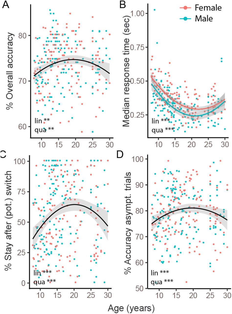
Task performance across age. Each dot shows one participant, color denotes sex. Curves show best-fitting regression models, including linear and quadratic effects of age. Shaded areas show standard errors of the mean regression line. “Lin.”: significant linear contrast (liner change with age); “qua.”: significant quadratic contrast (U-shaped or inverse-U-shaped change with age). Stars denote p-values (* p<.05, ** p<.01, *** p<.001). (A) Percentage of correct choices across the entire task (120 trials). (B) Median response times on correct trials. Regression coefficients differed significantly between males and females and are shown separately. (C) Fraction of stay trials after (potential, “pot.”) switches (red arrows in Fig. 1C). (D) Accuracy on asymptotic trials (grey bars in Fig. 1C).
Using (logistic) mixed-effects regression (methods in section Behavioral Analyses; results in Table 1), we found positive linear and negative quadratic age contrasts in all three performance measures. This reveals that the shape of age trajectories was dominated by monotonic performance improvements in combination with a performance peak in mid-adolescents (Fig. 2A, C, D; Table 1).
To identify the age of peak performance suggested by the quadratic effect, we assessed the binned data. In accordance with our hypothesis, the peak occurred in the intermediate age range, such that 13-to-15-year-olds outperformed both younger participants (8-13) and adults (18-30) on several measures of task performance. In terms of overall accuracy, performance peaked in 13-to-15-year-olds and declined steeply for both younger and older participants (Fig. 3C). 13-to-15-year-olds were also most willing to repeat previous actions after a single negative outcome (“stay on (potential) switch trial”), especially compared to younger children (Fig. 3E). This suggests that 13-to-15-year-olds were most persistent in the face of negative feedback. Furthermore, 13-to-15-year-olds performed best during stable task periods, showing the highest accuracy on asymptotic trials, especially compared to younger participants (Fig. 3F; also see suppl. Fig. 8).
Behavioral and Age Effects of Positive versus Negative Outcomes
We next assessed the effects of positive and negative outcomes on behavior. 13-to-15-year-olds adapted their choices more optimally to previous outcomes than younger or older participants. To show this, we used mixed-effects logistic regression to predict actions on trial t from predictors encoding positive or negative outcomes on trials t − i, for delays 1 ≤ i ≤ 8 (for details, see section Behavioral Analyses). The effects of positive outcomes were several times larger than the effects of negative outcomes (suppl. Table 7; Fig. 8B-F), in accordance with the task structure: Positive outcomes were diagnostic, indicating with certainty that an action was correct, whereas negative outcomes were non-diagnostic, being ambivalent as to whether a switch occurred or not. This jus-tifies the strong effect of positive and the weak effect of negative outcomes on behavior. Crucially, this pattern showed prominent age effects, revealed by interactions between age and previous outcomes in the regression models (suppl. Fig. 8B, C, E, and F; suppl. Table 7). On trials t − 1 and t − 2, positive outcomes interacted with age and squared age (all p’s < 0.014; suppl. Table 7), showing that the effect of positive outcomes increased with age and then slowly plateaued (suppl. Fig. 8C, F). For negative outcomes, the signs of the interaction was opposite for trials t − 1 versus t − 2 (all p’s < 0.046; suppl. Table 7), showing that the effect of negative outcomes flipped, being weakest in 13-to-15-year-olds for trial t − 1 (Fig. 8F), but strongest for trial t − 2. In other words, 13-to-15-year-olds were best at ignoring single, ambivalent negative outcomes (t − 1), but most likely to integrate long-range negative outcomes (t − 2), which potentially indicate task switches.
To summarize our model-agnostic results, 13-to-15-year-olds outperformed younger participants, older adolescents, and adults on a stochastic and volatile task, which was designed to mimic environmental challenges specific to adolescence. We next used computational modeling to test hypotheses about the cognitive processes that might underlie these age differences, employing both RL and BI.
Cognitive Modeling
Winning RL Model
The winning RL model had four free parameters: persistence p, inverse decision temperature β, and learning rates α+ and α− for positive and negative outcomes, respectively (section Reinforcement Learning (RL) Models). The model had the ability to learn from counterfactual outcomes, but model fit was best when counterfactual learning was directly tied to factual learning rather than controlled by an additional free parameter, such that updates of the same size (but opposite signs) were applied to both chosen and unchosen actions, according to learning rates α+ for positive out-comes and α− for negative outcomes. Parameters p and β controlled the translation of RL values into choices: persistence p increased the probability of repeating choices (independently of choice value) when p > 0, and of alternating choices when p < 0, while β induced decision noise (increased probability of exploratory choices) when small, and allowed for reward-maximizing choices when large.
Winning BI model
In the BI framework, participants cast the task as having distinct hidden states, separated by reversals (e.g., “Left choice is correct” and “Right choice is correct”; Fig. 3A, right). Participants’ goal is to infer the current hidden state, by observing the outcomes (e.g., reward, no reward) to their actions (e.g., left, right), engaging a mental model that specifies how likely each outcome arises in response to each action in each hidden state, and how likely each hidden state transitions to each other. Once participants have formed a posterior belief about the current hidden state, combining the state likelihood with their prior state belief, they can select the action with the highest probability of reward in this state.
The winning BI model also had four parameters: choice-parameters p and β as in the RL model, as well as task volatility pswitch and reward stochasticity preward, which characterized participants’ internal model of the task (Fig. 3A; section Bayesian Inference (BI) Models). pswitch ranged from stable (pswitch = 0) to volatile (pswitch > 0), and preward ranged from deterministic (preward = 1) to stochastic (preward < 1). The actual task was based on pswitch = 0.05 and preward = 0.75, meaning that the optimal mental model of the task would employ these values.
Hierarchical Bayesian Model Fitting
We first conducted exhaustive model comparison to create a best-possible model of each type (RL and BI), assessing improvements caused by adding various previously-proposed model augmentations (for details, see section Reinforcement Learning (RL) Models). The winning models of both types showed superior numerical model fit in terms of WAIC scores (Watanabe, 2013) when compared to differently parameterized models or the same type (Table 2), and also validated better behaviorally, closely reproducing human behavior (Palminteri et al., 2017; Wilson and Collins, 2019; Fig. 3C, E, F; suppl. Fig. 11). The winning RL model had the overall lowest WAIC score, revealing best quantitative fit, but both models validated equally well qualitatively: Both showed human-like behavior, and reproduced all age differences in detail, including 13-to-15-year-olds’ performance peak (Fig. 3C), their peak in the proportion of staying after (potential) switch trials (Fig. 3E), in asymptotic performance on non-switch trials (Fig. 3F), and their most efficient use of previous out-comes to adjust future actions (suppl. Fig. 8 D-F). Other models did not capture all these qualitative patterns (suppl. Fig. 11, 12).
The closeness in WAIC scores (Table 2), and especially the fact that both models were equally able to reproduce all crucial details of human behavior, show that both models captured human behavior adequately, and suggests that both might provide adequate explanations of the underlying cognitive processes. We therefore fitted both models to participant data to estimate individuals’ parameter values, using hierarchical Bayesian fitting (Fig. 3B; section Model Fitting and Comparison). We chose the hierarchical Bayesian method because it 1) recovered individual parameters better than classic maximum-likelihood fitting (suppl. Fig. 9); and 2) allowed us to estimate the effects of age on model parameters in a superior, statistically unbiased way (Katahira, 2016; M. D. Lee, 2011; van den Bos et al., 2017).

(A) Conceptual depiction of the RL and BI models. In RL (left), actions are selected based on learned values, illustrated by the size of stars (Q(left), Q(right)). In BI (right), actions are selected based on a mental model of the task, which differentiates different hidden states (“Left is correct”, “Right is correct”), and specifies the transition probability between them (p(switch)) as well as the task’s stochasticity (p(reward)). The sizes of the two boxes illustrate the inferred probability of being in each state. (B) Hierarchical Bayesian model fitting. Left box: RL and BI models had free parameters θRL and θBI, respectively. Individual parameters θj were based on group-level parameters θsd, θint, θlin, and θqua in a regression setting (see text on the right). For each model, all parameters were simultaneously fit to the observed (shaded) sequence of actions ajt of all participants j and trials t, using MCMC sampling. Right: We chose uninformative priors for group-level parameters; the shape of each prior was based on the parameter’s allowed range. For each participant j, each parameter 0 was sampled according to a linear regression model, based on group-wide standard deviation 0sd, intercept θint, linear change with age θlin, and quadratic change with age 0qua. Each model (RL or BI) provided a choice likelihood p(ajt) for each participant j on each trial t, based on individual parameters θj. Action selection followed a Bernoulli distribution (see Model Fitting and Comparison for details). (C)-(F) Human behavior for the measures shown in Fig. 2, binned in age quantiles. (C), (E), and (F) also show simulated model behavior for model validation, verifying that models closely reproduced human behavior and age differences.
Age Differences in Model Parameters
Our analyses revealed that several parameters changed with age (Fig. 4; suppl. Tables 10 and 11). In both the RL and BI model, choice parameters p and β increased monotonically with age, growing rapidly at first and plateauing around early adulthood (Fig. 4A, B, E, F). The age-based fitting model (section Model Fitting and Comparison) revealed that both the initial linear increase and later change in slope were significant, showing significant linear and negative quadratic effects of age for both parameters (suppl. Table 10). This shows that in this task, participants’ willingness to repeat previous actions independently of previous outcomes (p), and to exploit the best known option (β), steadily increased until adulthood, with steady growth during the teen years. Parameters p and β were thereby almost perfectly correlated between the RL and BI model (parameter p: Spearman p = 0.97, p < 0.05; parameter β: p = 0.94, p < 0.05; Fig. 5B), even though both models were fitted independently. This suggests that choice parameters captured robust, update-independent aspects of decision making.

Fitted model parameters for the winning RL (left column) and BI model (right), plotted over age. Stars indicate significant linear (“lin”) and quadratic (“qua”) effects of age on model parameters, based on the age-based fitting model, and differences between age groups, based on the age-less fitting model (section Model Fitting and Comparison; suppl. Tables 10 and 11). Dots (means) and error bars (standard errors) show the results of the age-less fitting model, providing an unbiased representation of individual fits. (A)-(D) RL model parameters. (E)-(H) BI model parameters.

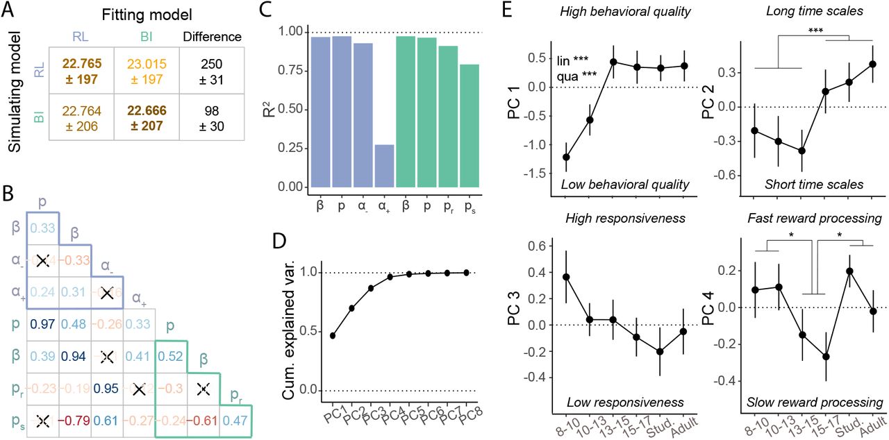
Relating RL and BI models. (A) Model recovery. WAIC scores were worse (larger; lighter colors) when recovering behavior that was simulated from one model (row) using the other model (column), than when using the same model (diagonal), revealing that the models were discriminable. The difference in fit was smaller for BI simulations (bottom row), suggesting that the RL model captured BI behavior better than the other way around (top row). (B) Spearman pairwise correlations between model parameters. Red (blue) hue indicates negative (positive) correlation, saturation indicates correlation strength. Non-significant correlations are crossed out (Bonferroni-corrected at p = 0.00089). Light-blue (teal) letters refer to RL (BI) model parameters. Light-blue / teal-colored triangles show correlations within each model, remaining cells show correlations between models. (C) Variance of each parameter explained by parameters and interactions of the other model (“R2”), estimated through linear regression. All four BI parameters (green) were predicted almost perfectly by the RL parameters, and all RL parameters except for α+ (RL) were predicted by the BI parameters. (D)-(E) Results of PCA on model parameters. (D) Cumulative variance explained by all principal components PC1-8. The first four components captured 96.5% of total parameter variance. (E) Age-related differences in PC1-4: PC1 reflected overall behavioral quality and showed rapid development between ages 8-13, which were captured by linear (“lin”) and quadratic (“qua”) effects in a regression model. PC2 captured a step-like transition from shorter to longer updating time scales at age 15, as revealed by PC-based model simulations (Supplements). PC3 showed no significant age effects. PC4 captured the variance in a+ and differed between adolescents 15-17 and both 8-13 year olds and adults. PC2 and PC4 were analyzed using t-tests. * p < .05; ** p < .01, *** p < .001.
Other parameters showed non-monotonic age trajectories. α−, preward, and pswitch declined drastically between ages 8-10 and 13-15, but then reversed their trajectory and increased again, reaching a slightly lower plateau around 15-17 years, which lasted through adulthood (Fig. 4C, G-H). For α− and preward, these changes were captured in significant pairwise differences between 8-to-10-yearolds and 13-to-15-year-olds, as well as between 13-to-15-year-olds and adults (25-30; for statistics, see suppl. Table 11), tested using the age-less fitting model (Model Fitting and Comparison). For pswitch, age differences were captured in a significant quadratic effect of age in the age-based model (suppl. Table 10).
Because the mental model in the BI model mirrored the true task structure, participants’ model parameters can be compared to the task’s true underlying parameters (preward = 0.75; pswitch = 0.05) to determine the optimality of the mental model. In accordance with the behavioral peak, both parameters were most optimal in 13-to-15-year-olds, whereas 8-to-10-year-olds and adults (18-30) fundamentally overestimated task volatility (pswitch), while underestimating reward stochasticity (preward). Even though the RL model does not afford assessment of optimality, lower learning rates from negative feedback α− are beneficial in this task because they allow to avoid premature switching based on single negative outcomes, while allowing for adaptive switching after multiple negative outcomes. In correspondence with our behavioral findings, a− was lowest in 13-to-15-year-olds.
Parameter α+ showed a unique stepped age trajectory, featuring relatively stable values through-out childhood and adolescence (8-17), but a sudden increase in adults (18-30; Fig. 4D). To summarize our modeling results, all 4 computational parameters in each model contributed to the age-related differences in behavior exhibited by participants and reproduced by the models. This shows that the non-linear trajectory of task performance can be explained by an interplay of trajectories in the underlying parameters, including monotonic growth (p, β), U-shaped trajectories (α−, preward, pswitch), and a step function (α+). Both an explanation in terms of changes in learning, with a crucial distinction between learning from positive and negative outcomes (RL model), and an explanation in terms of mental models, with a non-linear trajectory of optimality (BI model), might appropriately explain participants’ developmental trajectory in probabilistic switching.
Integrating RL and BI Model Findings
This result raises several questions: Why do both models, RL and BI, capture human behavior? Do both capture the same aspects of behavior, or different ones? Do the cognitive processes each invokes differ from each other fundamentally, or do they actually describe similar processes, simply using different terms? And lastly, can the use of both models lead to insights that could not have been gained from one model alone? The following section addresses these questions, conducting a generate-and-recover procedure to determine whether models were identifiable; assessing the correlations between the parameters of both models; determining how much variance in each parameter was explained by the parameters of the other model; and evaluating the dimensions of largest variance that arose in the shared space of both models.
Model Identifiability
For the generate-and-recover model-recovery procedure, we simulated artificial behavior from each model and assessed how well the opposite model fit these data. We used human-fitted parameter values for simulation to ensure that simulated behavior occupied a meaningful range (Heathcote et al., 2015; Wilson and Collins, 2019). This analysis can shed light on whether both models captured the same or distinct aspects of behavior: If models are identifiable, i.e., the simulated behavior of each model is better fitted by the corresponding model than the other one, that means that the models generated and captured different aspects of behavior, making them distinguishable. For example, in a situation in which the RL model fits the RL data best, and the BI model fits the BI best, both generated and captured distinguishable behaviors. If models are not identifiable, on the other hand, i.e., simulated behavior of each model is fitted equally well by both models, both potentially generated and captured the same variance in behavior; in this case, it is not possible to draw conclusions from model comparison. We found that both models were identifiable (Fig. 5A), showing that each captured unique aspects of behavior. Interestingly, the difference in fits was smaller when fitting the RL model (left column in Fig. 5A), suggesting that the RL model captured more aspects of BI behavior than the other way around, potentially reflecting increased versatility of this model.
Relations between Parameters
We next asked whether both models captured similar cognitive mechanisms, despite their differences in form.
To answer this question, we first determined how closely individual parameters were related between models, assessing pairwise Spearman correlations. As mentioned before, parameters p and β were almost perfectly correlated between models, suggesting high similarity of choice processes between models (Fig. 5B). Furthermore, parameter preward (BI) was strongly correlated with α− (RL), suggesting that beliefs about task stochasticity and negative learning rates played similar roles in both models, presumably in the integration of negative outcomes. The other mental-model parameter, pswitch (BI), was strongly negatively correlated with β (RL), suggesting that beliefs about task volatility in the BI model captured aspects that were explained by decision noise in the RL model. This is consistent with the notion that an expectation of high task volatility could be mistaken for increased choice stochasticity. The only parameter that showed no large correlations with other parameters was α+ (RL), potentially reflecting a cognitive process unique to the RL model. Taken together, some parameters likely captured similar cognitive processes in both models, exemplified by large correlations across participants. These similarities arose despite differences in the functional form of both models. On the other hand, models also showed unique parameters, potentially reflecting more unique cognitive processes.
The previous analysis showed that both models captured similar processes using different individual parameters, but similar processes might also be captured in the interplay between several parameters. To investigate this possibility, we next used linear regression to evaluate how well we could predict each parameter based on the parameters and one-way parameter interactions of the other model. This analysis revealed that 7 of 8 parameters could be predicted almost perfectly (Fig. 5C), showing that the interplay between parameters in one model captured almost all variance in almost every parameter in the opposite model. In other words, fitting the RL model on participants’ data allowed us to nearly perfectly predict participants’ BI parameters, without fitting the BI model. Parameter α+ (RL) was again an exception, with only small amounts of variance captured by BI parameters, suggesting that it reflected mechanisms that were unique to the RL model. These mechanisms might increase the versatility of the RL model, and possibly account for the slightly better numerical fit of the RL model to human (Table 2) and simulated data (Fig. 5A). In sum, in addition to significant similarities between individual parameters, the RL and BI models showed even greater similarities in terms of cognitive processes that were captured in the interactions between multiple parameters. This suggests that both models captured very similar cognitive processes, albeit without reaching identity (e.g., parameter α+).
Distilling Model Parameters Using PCA
Based on the fact that each model captured unique aspects of behavior and employed unique cognitive processes, we lastly aimed to determine what we could deduce from both models combined that we could not deduce from each alone. To this end, we used PCA to unveil lower-dimensional structure embedded in the 8-dimensional parameter space created by both models (section Principal Component Analysis (PCA)). We found that the first four principle components (PCs) of the PCA explained almost all variance (96.5%; Fig. 5D), showing that individual differences in all 8 parameters could be summarized by differences in just 4 dimensions. Succinctly summarizing both computational models, these 4 PCs provide a compressed and information-rich representation of the cognitive process, which has the potential to further illuminate the trajectory of cognitive development.
Our next goal therefore was to understand these PCs. The standard approach to interpreting PCs is to investigate which raw features (in our case, model parameters) were combined with which weights (factor loadings) to produce each PC (section Principal Component Analysis (PCA)). In our case, this approach was impeded by the fact that some model parameters—specifically RL learning rates—are inherently difficult to interpret because their roles are influenced by many factors, including the underlying task (Eckstein et al., n.d.) and computational model (Sugawara and Katahira, 2021), which makes them less suitable to anchor the meaning of PCs. To resolve this issue, we devised a novel method to understand the PCs in our study: Because PCs were linear combinations of model parameters, we could directly simulate the effects each PC had on behavior by simulating datasets with the corresponding model parameters, using our RL and BI models (for details, see section Principal Component Analysis (PCA)). Specifically, we simulated datasets with particularly big and particularly small values of each PCs (suppl. Fig. 13A). Assessing the behavior of these extreme cases provides detailed insight into the specific roles of each PC, and can—in turn—aid the interpretation of model parameters. More details are provided in section ??.
Our analysis revealed that PC1, capturing the largest proportion of variance in the dataset, reflected a broad measure of behavioral quality. This was evident in the low performance and lack of distinction between reward histories for the datasets that were simulated based on low values of PC1, and the high performance and optimal response to reward histories in the datasets based on high values of PC1 (suppl. Fig. 13A, left and right; suppl. Table 12; suppl. Text). Factor loadings revealed that low behavioral quality was caused by larger-than-average values of α− (RL), which likely led to premature switching, and preward and pswitch (BI), which created overly deterministic and volatile mental models of the task (suppl. Fig. 13A, center). High behavioral quality, on the other hand, was caused by larger-than-average values of α+ (RL), which likely facilitated the quick integration of positive outcomes; p (RL and BI), which increased choice persistence; and β (RL and BI), which reduced decision noise.
PC2, which explained the second-most variance after PC1, represented integration time scales. Simulated behavior based on low values of PC2 exemplified overly-short time scales, reflected in pronounced win-stay behavior—i.e., immediate switching after negative outcomes and consistent staying after positive outcomes—, which led to suboptimal performance on asymptotic trials (suppl. Fig. 13B, left). High values of PC2, on the other hand, led to overly-long time scales, such that every behavioral change took a long time, leading to suboptimally-slow behavioral switches (suppl. Fig. 13B, right). Overly-short time scales were driven by larger-than-average values of α+ and α− (RL), which led to a reliance of learning on just the most recent outcomes; mental models that are above-average volatile (pswitch) and extremely deterministic (preward), i.e., the belief that every correct action is rewarded and hidden states switch permanently; and larger-than-average values of p (RL and BI), which lead to a prevalence of outcome-independent choice repetitions.
PC3 captured responsiveness to task outcomes. Low responsiveness was characterized by a lack of differentiation between outcome histories and slow behavioral switching (suppl. Fig. 13C, right), whereas high responsiveness was characterized by extremely consistent win-stay-lose-shift behavior (suppl. Fig. 13C, left). Behavior with low responsiveness was caused by larger-than-average values of p, which favors outcome-independent choices; and pswitch, which leads to the belief that the task is constantly switching. Behavior with high responsiveness was caused by larger-than-average values of β, which effectively made task experience the only factor that determined choices; and larger-than-average values of preward, which institute the belief that every correct action is rewarded.
PC4 was dedicated to the unique RL parameter α+, capturing the tension between slow and fast updates from positive outcomes (suppl. Fig. 13D).
Three of these four PCs showed prominent age effects, suggesting that the PCA can provide an additional window into cognitive development in our task. PC1 (behavioral quality) was very low in the youngest age group (8-10 years), but increased drastically until age 13, at which it reached a stable plateau that lasted throughout adulthood (Fig. 5E, top-left). Regression models revealed significant linear and quadratic effects of age (lin.: β = −0.47, t = −4.0, p < 0.001; quad.: β = 0.011, t = 3.43, p < 0.001), with no effect of sex (β = 0.020, t = 0.091, p = 0.93). This shows that one side of the inverse U-shape we observed in overall task performance (Fig. 2; suppl. Fig. 8; Fig. 3C-F) might be caused by age differences in behavioral quality: Thirteen-to-15-year-olds had reached adult levels of behavioral quality, while younger participants showed noisier, less focused, and less consistent behavior, potentially related to relatively less experience with computerized tasks, psychological experiments, and assessments of performance.
Nevertheless, PC1 could not explain the other side of the inverse U-shape in overall task performance, i.e., how 13-to-15-year-olds outperformed older teenagers (15-17) and adults (18-30). The key to this question might lie in PC2 (updating time scales): PC2 showed a step function, such that participants aged 8-15 acted on short times scales, whereas participants aged 15-30 acted on long time scales (Fig. 5E, top-right). A post-hoc t-test revealed that the difference between both groups was significant (t(266.2) = 3.44, p < 0.001). This pattern is in accordance with the interpretation that shorter time scales, facilitating rapid behavioral switches (suppl. Fig. 13B, left), were more beneficial for the current task than longer time scales, which impeded them (suppl. Fig. 13B, right). Times scales might therefore represent the determining factor that allowed 13-to-15-year-olds to outperform older participants.
PC4 (positive updates) differentiated the larger group of 13-to-17-year-olds from both younger (8-13) and older (18-30) participants (Fig. 5E, bottom-right), as revealed by significant post-hoc, Bonferroni-corrected, t-tests (8-13 vs 13-17: t(176.8) = 2.28, p = 0.047; 13-17 vs 18-30: t(176.6) = 2.49, p = 0.028). In other words, after accounting for variance in PCs 1-3, the remaining variance was explained by 13-to-17-year-olds’ relatively longer updating timescales for positive outcomes, meaning that positive outcomes had relatively weaker immediate, but stronger long-lasting effects. Even though longer positive time scales might play a role in 13-to-15-year-olds’ remarkable task performance, they are unlikely the only explanation because they did not distinguish 13-to-15-year-olds from 15-to-17-year-olds.
Discussion
Across species, the adolescent transition from childhood to adulthood brings great challenges for learning and exploration. These challenges may have caused the adolescent brain to evolve behavioral tendencies that promote adaptive learning in rapidly changing, uncertain environments. To test this idea, we examined the choice behavior of a large sample of participants across a wide age range in a stochastic and volatile task, which we adapted from rodent studies (Tai et al., 2012).
Behavioral Results
Indeed, 13-to-15-year-olds performed better than both younger (8-13) and older participants, including adults (15-30): 13-to-15-year-olds achieved the highest overall accuracy, were most willing to wait out negative feedback, and made the best choices during stable task periods. 13-to-15-year-olds also used negative feedback most optimally to guide future choices, being least affected by proximal, but most sensitive to distal outcomes. This shows an ability to ignore ambivalent information while responding appropriately to meaningful patterns.
Whereas the developmental literature has long documented linear developments between childhood and adulthood, a recent focus on the period of adolescence has revealed an abundance of similar U-shaped trajectories, especially in the domain of neuro-cognitive and emotional processing (for reviews, see Dahl et al., 2018; Giedd et al., 1999; Somerville and Casey, 2010; Sowell et al., 2003; Toga et al., 2006). Increasingly, evidence is accumulating that adolescents outperform adults in various domains, including probabilistic learning (Cauffman et al., 2010; Davidow et al., 2016), deterministic reversals (van der Schaaf et al., 2011), creativity (Kleibeuker et al., 2013), and social learning (Gopnik et al., 2017). Similar prowess in flexibility has also been reported in studies of developing rodents (Guskjolen et al., 2017; Johnson and Wilbrecht, 2011; Simon et al., 2013).
Modeling results
RL Model
To understand which cognitive and neural processes underlay these differences in task behavior, we created two types of computational models, RL and BI. To reproduce human behavior appropriately, the RL model required several augmentations: the ability to learn from counterfactual outcomes (updating values of non-chosen actions); different learning rates for positive and negative outcomes (α+ and α−); persistence, i.e., the tendency to repeat actions independently of their previous outcomes (p); and the classic decision temperature β, which allows for the exploration of non-maximizing actions. One reason that RL models have been used so extensively in the (clinical) cognitive neurosciences is the abundance of evidence that has linked RL computations to specific neural mechanisms in a specialized network of brain regions including basal ganglia, cortical, and limbic regions (for reviews, see Frank and Claus, 2006; D. Lee et al., 2012; Niv, 2009; O’Doherty et al., 2015; Schultz and Dickinson, 2000). Using RL modeling in developmental population there-fore holds the promise of shedding light not only on cognitive, but also brain development (e.g., Christakou et al., 2013; Davidow et al., 2016; Javadi et al., 2014; Master et al., 2020; for reviews, see Nussenbaum and Hartley, 2019; van den Bos et al., 2017). In our study, RL models showed that choice parameters (β, p) grew monotonically throughout childhood and adolescence, maturing in late adolescence or early adulthood. This is consistent with previous developmental modeling research (reviewed in Nussenbaum and Hartley, 2019), and with a role of late-developing brain circuits in choice behavior (Giedd et al., 1999; Gogtay et al., 2004; Nussenbaum and Hartley, 2019; Sowell et al., 2003; Toga et al., 2006). Nevertheless, our study provided a more detailed picture of the developmental trajectory than previous studies, showing a striking initial increase in the youngest participants, followed by an asymptote in late adolescence.
Whereas RL choice parameters have shown relatively consistent age trajectories across studies in the previous literature, there have been major inconsistencies for learning rate parameters (for review, see Nussenbaum and Hartley, 2019). In our study, learning rates from negative feedback (α−) showed a pronounced U-shape, with the lowest (most beneficial) values in 13-to-15-year-olds. Learning rates from positive feedback (α+), on the other hand, were stable throughout childhood and adolescence, then suddenly increased in adults. This suggests that one of the reasons why adolescents outperformed younger and older participants in the current task was that they responded more appropriately to the stochastic negative feedback, paying attention to consistent patterns and avoiding impulsive switches based on single outcomes.
Accordingly, previous studies have shown unique feedback processing in adolescents compared to younger and older participants (for review, see Lourenco and Casey, 2013). Nevertheless, whereas some previous studies have shown hypersensitivity to feedback, others have shown hypo-sensitivity, and some have found effects unique to positive feedback, while others were unique to negative feedback, or applied to both (e.g., Christakou et al., 2013; Davidow et al., 2016; Palminteri et al., 2016; van den Bos et al., 2009; for review, see Lourenco and Casey, 2013). These discrepancies make it difficult to link feedback processing to a single neural system across studies, and indeed, several systems have been suggested to underlie learning, including striatal incremental learning (Yagishita et al., 2014), hippocampal-based episodic memory (Bornstein and Norman, 2017; Wimmer et al., 2014), and frontal-cortical cognitive control (Badre et al., 2010; Collins and Frank, 2012; Daw et al., 2011). Evidence is also accumulating that the same model parameters can reflect different neuro-cognitive systems in different tasks when cognitive demands differ (Eckstein et al., n.d.; Nussenbaum and Hartley, 2019; but see Gershman, 2017; Gershman and Uchida, 2019; Starkweather et al., 2018 for a single-system account based on neural modulation). In accordance with these results, in our study, RL parameter a− showed similar developmental trajectories as BI parameters pswitch and preward, suggesting that α− might have taken on a mental-model-like role in planning behavioral switches, rather than reflecting the incremental, striatal-based learning many might expect from an RL learning-rate parameter (Schultz and Dickinson, 2000).
BI Model
Despite the large success and wide application of RL models in the (developmental) cognitive neurosciences (for reviews, see Frank and Claus, 2006; D. Lee et al., 2012; Niv, 2009; Nussenbaum and Hartley, 2019; O’Doherty et al., 2015; Schultz and Dickinson, 2000; van den Bos et al., 2017), it has recently been proposed that the BI framework is better suited to model reversal-learning tasks (Bartolo and Averbeck, 2020; Bromberg-Martin et al., 2010; Costa et al., 2015; Fuhs and Touretzky, 2007; Gershman and Uchida, 2019; Hauser et al., 2014; Izquierdo et al., 2017; Schlagenhauf et al., 2014; Solway and Botvinick, 2012). BI is often used as a model of inductive reasoning, i.e., the prediction of future events based on past regularities (Hume, 2008), and has been applied to a wide range of domains including categorical thinking (Goodman et al., 2008; Medin and Schaffer, 1978), word learning (Xu and Tenenbaum, 2007), causal reasoning (Griffiths and Tenenbaum, 2005), and creativity (Collins and Koechlin, 2012; for reviews, see Friston, 2009; Tenenbaum et al., 2011; also see special issue Chater et al., 2006). In addition, BI has become an indispensable tool in understanding cognitive development and learning, and BI models have even been proposed to reconcile the century-long debate between empiricist and nativist accounts of cognitive development (for examples, see special issue Gopnik and Tenenbaum, 2007). Even though they consist separate literatures, some inductive reasoning tasks have the same structure as stochastic reversal-learning tasks, presenting participants with observations that are generated from a noisy process, whose otherwise stable mean sometimes changes unexpectedly (e.g., Nassar et al., 2012; O’Reilly et al., 2013; Yu and Dayan, 2005). Like in our task, the challenge of these tasks lies in differentiating noisy observations during stable task periods from actual switches in the hidden state.
Due to their natural framing of volatile, stochastic environments (Chater et al., 2006; Friston, 2009; Gershman and Uchida, 2019; Izquierdo et al., 2017; Tenenbaum et al., 2011), and their huge promise for developmental research (Gopnik and Tenenbaum, 2007), we decided to fit a BI model to the current task, and compare it to the more established RL model. The BI model showed almost identical age trajectories of parameters β and p as the RL model, confirming that in our task, choice parameters increased monotonically through the second decade of life. BI mental model parameters—reward stochasticity preward and task volatility pswitch—, on the other hand, showed pronounced inverse-U trajectories, with most accurate values in 13-to-15-year-olds. This means that 13-to-15-year-olds possessed the most optimal mental model of the task (even though this model still deviated from Bayes-optimal behavior, being both too volatile and too deterministic). Children and adults treated the task as even more volatile and more deterministic than adolescents. For example, 8-to-13-year-olds behaved as if the task rewarded 92% of their correct responses, and adults as if it rewarded 91%, whereas 13-to-15-year-olds only expected rewards for 89% of their correct choices; in actuality, 75% of correct responses were rewarded.
Previous research has suggested that model parameters might be more accurately interpreted as cognitive “adaptation” rather than fixed “settings” (Nussenbaum and Hartley, 2019): Rather than reflecting a particular, developmentally-fixed state of the neural system (setting), parameters might instead reflect an ability of participants to adjust to specific task demands (adaptation; for a similar argument, see Davidow et al., 2016). In this light, our study suggests that adolescents have a unique ability to adapt to probabilistic (preward) and volatile environments (pswitch), showing an optimal response to negative feedback (a−).
PCA on Both Models
We next directly compared the RL and BI models to each other, and found that they captured both overlapping and unique behavioral patterns, and invoked both overlapping and unique cognitive processes (for detailed discussion, see section Benefits of Using Multiple Model Types). To combine the unique insights of both models, while stripping away redundancies, we performed a PCA on the parameters of both. This analysis revealed that general behavioral quality (PC1) improved steeply during childhood and early adolescence, and reached a stable plateau in 13-to-15-year-olds, which lasted through adulthood. Updating time scales (PC2), on the other hand, remained short during childhood and adolescence, including 13-to-15-year-olds, and only transitioned to adult levels thereafter. This suggests that 13-to-15-year-olds outperformed younger participants due to adult-like levels of behavioral quality (PC1), while outperforming adults due to child-like updating time scales (PC2). Reward processing (PC4) showed an inverse-U trajectory with minimum in 13-to-17-year-olds. Though this PC therefore cannot account for differences between 13-to-15-year-olds and 15-to-17-year-olds, it may contribute to differences between 13-to-15-year-olds and both children (8-13) and adults (18-30).
In conclusion, adolescents aged 13-15 likely performed so well on this task because they occupied a developmental “sweet spot” that combined mature levels of behavioral quality (PC1) with youthful times scales (PC2) and unique long-term updating of rewards (PC4). Though this combination would not be optimal in all environments (e.g., short time scales would be less beneficial if contexts switched less frequently), it was beneficial in our task, which supports the idea that the adolescent brain may pass through stages that have evolved to enhance success in stochastic and volatile environments.
Different Models at Different Ages?
Previous studies have shown that participants of different ages sometimes are better fitted by different computational models, suggesting that they might employ entirely different cognitive mechanisms at different ages (e.g., Palminteri et al., 2016). Could the same be the case in our study? For example, children’s cognitive processes might resemble a simple incremental RL model, whereas adolescents’ might approximate the mental-model-based—and more optimal—BI model. This out-come would be in accordance with the previously reported increase in “model-based” (compared to “model-free”) behavior with age (Decker et al., 2016), as well as with a reported increase in the tendency to employ counterfactual updating, which also reflects an improved mental task model (Palminteri et al., 2016). Even though this is a justified question, it is unlikely that different models applied to different age groups in our study, given that both models captured the behavior of all age groups equally well during model validation. Compared to previous studies that showed age differences in model types, the greater flexibility of our models in terms of the number of free parameters and other augmentations might have allowed them to capture more age differences, obliterating the need to change the model itself.
Previous Reversal-Learning Research in Adolescents
Even though reversal learning tasks have frequently been used in developmental samples (e.g., Boehme et al., 2017; Dickstein, Finger, Brotman, et al., 2010; Dickstein, Finger, Skup, et al., 2010; Finger et al., 2008; Harms et al., 2018), the development of reversal learning itself has received relatively little attention so far (Hauser et al., 2015; Javadi et al., 2014; van der Schaaf et al., 2011). One of the previous developmental studies (Javadi et al., 2014), comparing a large sample of 260 14-to-15-year-olds to 29 adults, did not show the same performance differences we found in our study. A likely reason is a crucial difference between task designs: whereas this study rewarded both correct (70%) and incorrect choices (40%), our study only rewarded correct choices (75%), but never incorrect ones (0%), making positive feedback perfectly diagnostic of correct choice (for study details, see suppl. Table 1). The behavioral benefits of adolescents we report here might therefore be contingent on the diagnosticity of positive feedback, a conclusion that is also supported by our PCA results (see section Integrating RL and BI Model Findings).
Another study compared a smaller sample of 19 adolescents across a wider age range (12-16 years) to 17 adults (Hauser et al., 2015), and also found no differences in overall task performance (see suppl. Table 2). This result, however, is in accordance with our study: with a U-shaped trajectory of performance, combining participants across the entire age range of 12-16 years will lead to a similar average as shown by adults. With respect to computational modeling, the study reported larger counterfactual negative learning rates in adolescents compared to adults, whereas we found the inverse. However, the study by Hauser et al. (2015) only provided limited model comparison, and did not validate the winning model against behavioral data, leaving open the possibility that model parameters did not adequately capture the observed behavior (Blohm et al., 2020; Palminteri et al., 2017; Wilson and Collins, 2019). In support of this conclusion, not just counterfactual negative learning, but all other learning parameters showed the same pattern of differences between adolescents and adults (Hauser et al., 2015, Fig. 2), and a similar model was previously found to generally fit adolescents worse than adults (Javadi et al., 2014), suggesting that differences in counterfactual negative learning were an unspecific artifact of other issues related to model fitting.
A third study (van der Schaaf et al., 2011) compared three groups of 15 adolescents each (10-17 years) to 16 adults (suppl. Table 1), thereby providing the only previous study that allowed treating age as a continuous variable, and therefore detecting potential U-shaped developments. Indeed, this study revealed the same inverse U-shape in performance on reversal trials as our study (Table 2; van der Schaaf et al., 2011, Fig. 3C). Despite differences in specific outcomes, both studies were also compatible in terms of adolescents’ unique learning patterns: While adolescents showed the most balanced reward-to-punishment learning in the Van der Schaaf et al. (2011), where rewards and punishments provided the same amount of information, they showed the most reduced learning from negative outcomes in our study, in which negative outcomes provided less information than positive outcomes. In other words, adolescents showed balanced learning in a task with balanced positive-to-negative feedback (van der Schaaf et al., 2011), but biased learning in a task with biased feedback (ours). Applying the lens of “adaptation” (Nussenbaum and Hartley, 2019) high-lights the consistency between both studies, and suggests that adolescents were more able to adapt to the specific settings of reversal tasks than children or adults.
Taken together, our study builds on and extends previous findings, showing that some developmental changes occur linearly, with a monotonic trajectory between childhood and adulthood (e.g., choice parameters β and p), whereas other changes are U-shaped, and show prominent peaks during adolescence (e.g., mental model parameters pswitch and preward; response to negative feedback a−). Previous group-based studies were unable to reveal these pattern in as much detail.
A Role of Puberty?
This study has shown that age makes a crucial difference in how participants make reward-based decisions in a volatile, stochastic environment. Nevertheless, we have not answered the question which biological mechanisms underlie these differences. There is growing evidence that gonadal hormones affect inhibitory neurotransmission, spine pruning, and other variables in the prefrontal cortex of rodents (Delevich et al., 2019; Delevich et al., 2018; Drzewiecki et al., 2016; Juraska and Willing, 2017; Piekarski, Boivin, et al., 2017; Piekarski, Johnson, et al., 2017), and evidence for puberty-related neurobehavioral change is also accumulating in human studies (Blake-more et al., 2010; Braams et al., 2015; Gracia-Tabuenca et al., 2021; Laube, van den Bos, et al., 2020; Op de Macks et al., 2016), suggesting that puberty-related changes in brain chemistry might be a mechanism behind the observed differences. To answer this question, we investigated how performance and model parameters changed with pubertal development—assessed through salivary testosterone levels (Master et al., 2020) and self-reported physical development (Petersen et al., 1988), This analysis revealed qualitatively similar patterns compared to age (suppl. Fig. 2,3,4; suppl. Tables 3, 4; for discussion, see suppl. Text). Nevertheless, pubertal measures were highly correlated with age (suppl. Fig. 1), making it difficult to identify puberty-specific effects. To investigate whether pubertal development had a unique effect after controlling for age, we also tested puberty effects within different age bins, but failed to reveal significant differences (suppl. Fig. 5, 6, 7). Nevertheless, some trends that emerged in the pubertal analyses, especially with respect to pre-pubertal participants, deserve a more detailed investigation in future research (section ??). Thus, pubertal development was unlikely a mechanism that underlay the observed age differences in the current study. A clear limitation of our study is that it was cross-sectional, rather than longitudinal. Future research with longitudinal designs might better address the potential role of puberty (Kraemer et al., 2000).
Results of t-tests on PC2 and PC4. df: Welch-adjusted degrees of freedom.
Benefits of Using Multiple Model Types
As mentioned above, it was one of our goals in this study to compare RL models—the standard in the learning and reversal literature—to BI models—claimed increasingly frequently to provide a better fit to reversal-learning tasks than RL models. We wanted to know if one model fit the data strictly better than the other; whether they captured different behavioral patterns; and whether they invoked different cognitive processes. To answer the two latter questions, we assessed simulated behavior from each model using the other model, determined whether parameters were correlated between models, and whether each parameter’s variance could be explained by the other model. All three analyses showed that the two models captured overlapping, but not fully identical behaviors, using overlapping, but not fully identical cognitive mechanisms. This shows that each model was unique, and that one could not be replaced by the other.
To answer the first question, we employed a broader approach to model comparison than most previous studies. Following the standard computational modeling approach, one type of cognitive model is selected (e.g., RL), and different variants of this type are compared to find the best-fitting one, which is then interpreted as the cognitive process employed by participants. The best-fitting model is identified using quantitative criteria of model fit such as Bayes factors (Mulder and Wagenmakers, 2016), minimum description length (Grünwald, 2007), or other appropriate measures of model fit that take model complexity into account (e.g. AIC, BIC, or here WAIC; Pitt and Myung, 2002; Watanabe, 2013). One problem with this approach is that it cannot rule out whether a model of a different type (e.g., BI) would fit the data better altogether. In the words of Nassar and Frank (2016), “the question always remains: could the data be better explained through a different set of mechanisms under a different set of assumptions?” This issue can be mitigated by verifying that the chosen model reproduces human behavior adequately, and is therefore a valid reflection of the observed data (Heathcote et al., 2015; Palminteri et al., 2017; Wilson and Collins, 2019), but only a small number of researchers adopt this practice consistently, so that we are often left wondering whether the “best-fitting” model actually captures the observed behavior.
Another concern with the standard approach, which is more difficult to address, is that different types of models frame behavior in terms of different cognitive processes, and one framing can be more informative, interpretable, appropriate to test the current hypothesis, concise, or in any other way better, than a different framing, and should therefore be chosen, potentially despite lower numerical model fit (Kording et al., 2020; Uttal, 1990; Webb, 2001): “The model that best fits your data may not be the best model” (Blohm et al., 2020). Identifying the “best” model based on such qualitative criteria is fundamentally difficult, and often based on researchers’ (explicitly stated or implicit) scientific goals (e.g., a preference for explanatory or predictive models; Bernardo and Smith, 2009; Navarro, 2019) and research philosophy (Blohm et al., 2020). The conclusion of decades of model building research is therefore that model selection needs to strike a balance between many aspects of model quality, including qualitative (e.g., generality, explanatory adequacy) and quantitative criteria (e.g., descriptive adequacy, complexity; Jacobs and Grainger, 1994). In other words, numerical model fit (e.g., BIC, AIC, WAIC) should never be used as the only criterion to assess model quality—good modeling practices take several criteria into account when assessing a model, including its qualitative fit to the data, generality, and explanatory power, amongst others.
Applying this approach, we found that both types of models—properly tuned—captured participant behavior in our task equally well. The numerical model fit (WAIC) favored the RL model over the BI model, but qualitative model validation showed that both models captured human behavior equally well (Palminteri et al., 2017). Model development and assessment of model quality can be based on “many potential criteria” (Blohm et al., 2020), which are equally valid, depending on the scientific question (Kording et al., 2020). In our case, the main motivation for the RL model was the continuity and comparability with previous research in the cognitive neurosciences, and specifically on the reversal-learning paradigm. We achieved this goal by creating an RL model that was continuous with previous research, uniting several previously proposed augmentations that had not been combined before, and achieving an overall better fit to the data. The main motivation for the BI model were numerous claims for its superiority compared to RL in our specific task (Gershman and Uchida, 2019; Izquierdo et al., 2017), and its promise in the cognitive (Tenenbaum et al., 2011), brain (Friston, 2009), and developmental sciences (Gopnik and Tenenbaum, 2007). Indeed, the BI model provided an immense advantage in terms of interpretability: BI model parameters directly mapped onto the concepts of interest for our research (stochasticity, volatility), promising a more direct window into their perception by participants. This highlights the important fact that each computational model offers just one of many possible interpretations of the underlying cognitive mechanism, and specifically, that many cognitive processes that have traditionally been explained in terms of RL could also be explained in terms of BI (or the other way around). Based on all these criteria, we concluded that both models, RL and BI, provided accurate, informative, and conclusive insights into our research questions, and that both should be interpreted with equal determination.
Fitting both models provided several benefits in understanding participants’ cognitive processes in our task: Both models provided converging as well as additive evidence. Converging results showed surprisingly strong, direct replication (β RL ↔ β BI, pRL ↔ pBI), and parallelism between different model parameters across models (preward, pswitch, α α −). Independent components led to additive insights (α+). In addition, each model’s conceptual framework and interpretation of the cognitive process became more distinctive in direct comparison with the other. For example, the parallelism between BI mental-model parameters and RL negative learning rate helped clarify the role of this otherwise ambiguous parameter. A final advantage of fitting both models was the possibility to investigate patterns that combined the insights of both models, going beyond any specific one, by using PCA on the shared parameter space. This analysis exposed a different set of factors, which differentiated 13-to-15-year-olds from younger participants (PC1), from older participants (PC2), and from both (PC4).
Conclusion
In conclusion, we used a simple task based on volatility and stochasticity to show that adolescents outperformed adults in a task that represented the kind of learning challenge that may have ecological validity to the transitions and challenges of adolescence. In our community sample, behavior was most optimal at age 13-15. We used two models to examine the underlying cognitive processes, based on RL and BI. The results suggest that adolescents achieved better performance for several reasons: (1) 13-to-15-year-olds lay on the right spot in a monotonic trajectory between childhood and adulthood (p and β). (2) 13-to-15-year-olds were outliers in terms of their ability to accurately assess the volatility and stochasticity of their environment, and in terms of their integration of negative outcomes (U-shapes in preward, pswitch, and α−). (3) 13-to-15-year-olds combined adult-like (PC1), child-like (PC2), and developmentally unique (PC4) strategies. These data suggest that multiple (neuro)cognitive systems might underlie developmental changes in brain function, at staggered time scales. Pubertal development and steroid hormones may impact a subset of these processes, yet causality is difficult to determine without manipulation or longitudinal designs (Kraemer et al., 2000).
For purposes of translation from the lab to the “real world”, our study indicates that how youth learn and decide changes in a nonlinear fashion as they grow. This underscores the importance of youth-serving programs that are developmentally informed and avoid a one-size-fits-all approach. Finally, these data support a positive view of adolescence and the idea that the adolescent brain exhibits remarkable learning capacities that should be celebrated.
Methods
Participants
All procedures were approved by the Committee for the Protection of Human Subjects at the University of California, Berkeley. We tested 312 participants: 191 children and adolescents (ages 8-17) and 55 adults (ages 25-30) were recruited from the community and completed a battery of computerized tasks, questionnaires, and saliva samples (Master et al., 2020); 66 university undergraduate students (aged 18-50) completed the four tasks as well, but not the pubertal-development questionnaire (PDS; Petersen et al., 1988) or saliva sample. Community participants were prescreened for the absence of present or past psychological and neurological disorders; the undergraduate sample indicated the absence of these. Compensation for community participants consisted in 25$ for the 1-2 hour in-lab portion of the experiment and 25$ for completing optional take-home saliva samples; undergraduate students received course credit for participation in the 1-hour study.
Exclusion Criteria
Out of the 191 participants under 18, 184 completed the current task; reasons for not completing the task included getting tired, running out of time, and technical issues. Five participants (mean age 10.0 years) were excluded because their mean accuracy was below 58% (chance: 50%), an elbow point in accuracy, which suggests that they did not pay attention to the task. This led to a sample of 179 participants under 18 (male: 96, female: 83). Two participants from the undergraduate sample were excluded because they were older than 30, leading to a sample aged 18-28; 7 were excluded because they failed to indicate their age. This led to a final sample of 57 undergraduate participants (male: 19, female: 38). All 55 adult community participants (male: 26, female: 29) completed the task and were included in the analyses, leading to a sample size of 179 participants below 18, and 291 in total (suppl. Fig. 1).
Quantile Bins
For some analyses, we split participants into quantiles based on age. This way of data binning led to samples of adequate sizes for summary statistics, and balanced group sizes after exclusion. Quantiles were calculated separately within each sex.
Testing Procedure
After entering the testing room, participants under 18 years and their guardians provided informed assent and permission; participants over 18 provided informed consent. Guardians and participants over 18 filled out a demographic form. Participants were led into a quiet testing room in view of their guardians, where they used a video game controller to complete four computerized tasks. At the conclusion of the tasks, participants between 11 and 18 completed the PDS questionnaire themselves and were measured in height and weight. Participants were then compensated with $25 Amazon gift cards.
Experimental Design
The task described in this work was the last of the four tasks. The other tasks will be or have been reported elsewhere (Master et al., 2020; Xia et al., 2020). The goal of this task was to collect golden coins, which were hidden in one of two green boxes. On each trial, participants decided which box to open, and task contingencies switched unpredictably throughout the task (Fig. 1B). Before the main task, participants completed a 3-step tutorial: A first prompt explained that one of the two boxes contained a coin (was “magical”), whereas the other one did not. Ten practice trials followed on which one box revealed a coin when selected, whereas the other was empty (deterministic tutorial). The second prompt stated that the magical box would sometimes switch sides. Participants then received eight trials on which the second box contained the coin (but not the first), followed by eight more trials on which the first box contained the coin (but not the second; switching tutorial). The third and last prompt explained that even the magical box did not always contain a coin. This prompt directly led into the main task (stochastic switching), with 120 trials.
In the main task, the correct box was rewarded in 75% of trials; the incorrect box was never rewarded. After participants reached a performance criterion (see below), it became possible for contingencies to switch (without notice), such that the previously incorrect box was now the correct one. The performance criterion was to collect 7-15 rewards, whereby the specific number was pre-randomized for each block. Any number of non-rewarded trials was allowed in-between rewarded trials. Due to this design, switches only occurred after rewarded trials. For consistency with the rodent version of the task (Tai et al., 2012), the first correct choice after a switch was always rewarded (while retaining an average of %75 probability of reward for correct choices).
Behavioral Analyses
We assessed the effects of age on behavioral outcomes (Fig. 2), using (logistic) mixed-effects regression models with the package lme4 (Bates et al., 2015) in R (RCoreTeam, 2016). All models included the following set of regressors to predict outcomes of interest (e.g., overall accuracy, response times): Age, to assess the linear effect of age on the outcome; squared age, to assess the quadratic (U-shaped) effect of age; and sex; furthermore all models specified random effects of participants, allowing participants’ intercepts and slopes to vary independently. When models included additional predictors, this is noted in the main text.
We assessed the effects of previous outcomes on participants’ choices (suppl. Fig. 8B, C, E, F) using a logistic mixed-effects regression model, which predicted actions (left, right) from previous outcomes (details below), while testing for effects of and interactions with sex, z-scored age, and z-scored quadratic age, specifying participants as mixed effects. We included one predictor for positive and one for negative outcomes at each delay i with respect to the predicted action (e.g., i = 1 trial ago). Outcome predictors were coded -1 for left and +1 for right choices, and 0 otherwise. Including predictors of trials 1 ≤ i ≤ 8 provided the best model fit (suppl. Table 7). To visualize the results of this grand regression model (including all participants), we ran a separate model for each participant with the same structure, and show individual fits in suppl. Fig. 8B, C, E, F.
Computational Models
Reinforcement Learning (RL) Models
In RL, decisions are made based on action values, which are continuously updated based on outcomes (Sutton and Barto, 2017). A simple RL model has two parameters, learning rate α and decision temperature β. On each trial t, the value Qt(a) of action a is updated based on the observed outcome ot ∊ [0, 1] (reward, no reward), in the following way:
 This means that previous action values are updated in proportion to the difference between the estimated value and the actual reward, scaled by the learning rate a. The difference itself, ot − Qt(a), is called “reward prediction error”.
Over time, action values approximate the true underlying reward probabilities. Decisions are based on these values by calculating action probabilities using a softmax transform:
 Here, a is the selected, and αns the non-selected action.
The best-fit 4-parameter RL model was based on this 2-parameter model, with additional parameters learning rate for negative outcomes α −, persistence p, as well as counterfactual reasoning (see below). Adding α − allowed for separate updates of rewarded (ot = 1) and non-rewarded (ot = 0) trials: Qt(a) = Qt(a) + α +(ot − Qt(a)) iff ot = 1, and Qt(a) = Qt(a) + a−(ot − Qt(a)) iff ot = 0, with independent a− and a+. Choice persistence or “stickiness” p changed the value of the previously-selected action at on the subsequent trial, biasing toward staying (p > 0) or switching (p < 0): Q(at) = Q(at) + p iff at = at−1.
Counterfactual reasoning was implemented through updates to the values of non-selected actions, using counterfactual outcomes 1 − ot: Qt+1(ans) = Qt(ans) + α +((1 − ot) − Qt(ans)) iff o = 1, and Qt+1(ans) = Qt(ans) + a−((1 − ot) − Qt(ans)) iff o = 0. Initially, we used four parameters α +, α +c, α −, and α−c to represent each combination of value-based (“+” versus “-”) and counter-factual (“c” versus factual) updating, but collapsing α + = α +c and α − = α −c improved model fit (Table 2). This suggests that outcomes triggered equal-sized updates to chosen and unchosen actions. Explained differently, the final model based decisions on a single value estimate—the value difference between the two available actions—, rather than on independent value estimates for each. Chosen and unchosen actions were updated to the same degree and in opposite directions on each trial.
Action values were initialized at 0.5 for all models, reflecting equal initial values for the two actions.
Bayesian Inference (BI) Models
The BI model assumes that participants know that the task has two latent states: “Left action is correct” (aleft = cor) and “Right action is correct” (aright = cor), where cor stands for correct (inc: incorrect). Participants assume that on each trial, the latent state switches with probability pswitch, and that in each state, the probability of receiving a reward for the correct action is preward (Fig. 3A). On each trial, participants select an action in two phases, using the Bayesian Filter algorithm (Sarkka, 2013): (1) In the estimation phase, participants infer the hidden state of the previous trial t − 1, based on the outcome ot−1 they received for their action at−1, using Bayes rule:
 p(at−1 = cor) is the prior probability that at−1 was correct (on the first trial, p(a = cor) = 0.5 for both actions), and p(ot−1 │ at−1) is the likelihood of the observed outcome ot−1 given action at−1. According to the mental model, likelihoods are (dropping underscripts for clarity): p(o = 1 a = cor) = preward, p(o = 0 a = cor) = 1 − preward, p(o = 1 a = inc) =, and p(o = 0 │ a = cor) = 1 −, where is the probability of receiving a reward for an incorrect action, which was 0 in reality, but we set = 0.0001 to avoid model degeneracy.
(2) In the prediction phase, participants integrate the possibility of state switches by propagating the inferred knowledge about the hidden state at t − 1 forward to trial t:
 We first assessed a parameter-free version of the BI model, truthfully setting preward = 0.75, and pswitch = 0.05. Lacking free parameters, this model was unable to capture individual differences and led to poor qualitative (suppl. Fig. 12A) and quantitative model fit (Table 2). The best-fit BI model had four free parameters: preward and pswitch, as well as the choice parameters β and p, like the winning RL model. β and p were introduced by applying a softmax to p(at = cor) to calculate p(a), the probability of selecting action a on trial
  . When both actions had the same probability p(a) and persistence p > 0, then staying was more likely; when p < 0, then switching was more likely.
Model Fitting and Comparison
We fitted parameters using hierarchical Bayesian methods (Katahira, 2016; M. D. Lee, 2011; Fig. 3B), and found that the obtained results clearly superseded those of classical maximum-likelihood fitting in terms of parameter recovery (suppl. Fig. 9). Rather than fitting individual participants, hierarchical Bayesian model fitting estimates the parameters of an entire population jointly, by maximizing the posterior probability p(θ │ data) of all parameters θ conditioned on the observed data, using Bayesian methods:
 The unique feature of hierarchical Bayesian model fitting is that individual parameters are embedded in a hierarchical structure of priors, which helps resolve uncertainty at the individual level.
We ran two models to fit parameters: The “age-less” model was used to estimate individuals’ parameters in the least biased way and conduct binned analyses on parameter differences; the “age-based” model was used to statistically assess the shapes of parameters’ age trajectories. In the age-less model, each individual j’s parameters  or
or  were drawn from group-wide prior parameter distributions. Parameter β was drawn from a prior Gamma distribution, p from a prior Normal distribution, and α+, α−, preward, and pswitch from prior Beta distributions, in accordance with each parameter’s allowed range of values. The hyperpriors of these distributions are shown in suppl. Table 8.
Each individual’s parameters θj were entered into the RL or BI model, with the goal of determining both the group-level and individual parameters with the largest posterior probability under the behavioral data p(θ | data). Because p(θ |data) was analytically intractable, we approximated it using Markov-Chain Monte Carlo sampling, using the no-U-Turn sampler as implemented in the PyMC3 package in python (Salvatier et al., 2016). We ran 2 chains per model with 6,000 samples per chain, discarding the first 1,000 as burn-in. All models converged with small MC errors, sufficient effective sample sizes, and  close to 1 (suppl. Table 9). For model comparison, we used the Watanabe-Akaike information criterion (WAIC), which estimates the expected out-of-sample prediction error using a bias-corrected adjustment of within-sample error (Watanabe, 2013).
To obtain each participant’s individual fitted parameters, we calculated the means over all posterior samples in the age-less model, as shown in Fig. 4 and suppl. Figures 10, 11, and 12. To test whether a parameter 0 differed between two age groups a1 and a2, we determined the number of MCMC samples in the age-less model in which the parameter was larger in one group than the other, i.e., the expectation IE(θa1 < θa1) across MCMC samples. Following statistical convention, p < 0.05 was used to determine significance.
The age-less model was necessary to show individual parameters in the least biased way, given that this model did not have access to participants’ ages. To statistically assess the continuous effects of age on model parameters, we conducted a separate model in which model parameters were allowed to change depending on participants’ ages (Fig. 3B). This model was only used to statistically assess the shapes of parameters’ age trajectories, and not to estimate individuals’ parameters because individual parameters would be biased by the inclusion of age in the hierarchical structure of the model.
In the age-based model, each parameter 0 of each participant j was sampled from a Normal distribution around an age-based regression line (Fig. 3B):
 Each parameter’s intercept θint, linear change with age θlin, quadratic change with age θqua, and standard deviation around the regression line θsd were sampled from prior distributions of the form specified in suppl. Table 8.
Comparing RL and BI Models
Generate-and-Recover Procedure (Fig. 5A)
We simulated one dataset per participant from each model (RL and BI), using the model parameters fitted for the participant using the age-free fitting method. We then fitted the simulated data with the RL and BI model, again using the age-free method. We finally calculated WAIC scores and standard errors using PyMC3 (Salvatier et al., 2016).
Correlations between Model Parameters (Fig. 5B)
We used Spearman correlation, the nonparametric version of the Pearson product-moment correlation, because parameters followed different, not necessarily normal, distributions. Employing Pearson correlation led to similar results. p-values were corrected for multiple comparisons using the Bonferroni method.
Predicting Parameters from Parameters of the Other Model (Fig. 5C)
We ran eight different regression models, predicting each parameter from the four parameters of the opposite models, as well as their one-way interactions, using linear regression in R (RCoreTeam, 2016). Fig. 5C shows the explained variance (R2) of each model.
Principal Component Analysis (PCA)
To extract components that covary across parameters, we ran PCA on the fitted parameters data (8 parameters per participant). PCA can be understood as a method that rotates the initial coordinate system of a dataset (in our case, 8 axes corresponding to the 8 parameters), such that the first axis is aligned with the dimension of largest variation in the dataset (first principle component; PC), the second axis with the dimension of second-largest variance (second PC), while being orthogonal to the first, and so on. In this way, all resulting PCs are orthogonal to each other, and explain subsequently less variance in the original dataset. We conducted a PCA after centering and scaling (z-scoring) the data, using the statistical programming language R (RCoreTeam, 2016).
Age Differences in Principle Components (PCs; Fig. 5E)
For each PC, we ran similar regression models as for our behavioral measures of performance, predicting participants’ PCs from age (linear), age (quadratic), and sex. When significant, effects were noted in Fig. 5E. For PC2 and PC4, we also conducted post-hoc t-tests, correcting for multiple comparison using the Bonferroni method (Table 3).
Acknowledgments
Numerous people contributed to this research: Amy Zou, Lance Kriegsfeld, Celia Ford, Jennifer Pfeifer, Megan Johnson, Gautam Agarwal, Liyu Xia, Vy Pham, Rachel Arsenault, Josephine Christon, Shoshana Edelman, Lucy Eletel, Neta Gotlieb, Haley Keglovits, Julie Liu, Justin Morillo, Nithya Rajakumar, Nick Spence, Tanya Smith, Benjamin Tang, Talia Welte, and Lucy Whitmore. We are also grateful to our participants and their families. The work was funded by National Science Foundation SL-CN grant 1640885 to RD, AGEC, and LW.
Footnotes
This version of the manuscript has been revised to update the introduction and discussion in light of a broader literature, and to clarify the computational approach taken in the manuscript.
References


