

Abstract
Forming transformation-tolerant object representations is critical for high-level primate vision. Although single cell neural recording studies predict the existence of highly consistent object representational structure across transformation in high-level vison, this prediction has not been tested at the population level. Here, using fMRI pattern analysis, we show that high representational consistency across position and size changes indeed exists in human higher visual regions. Moreover, consistency is lower in early visual areas and increases as information ascends the ventral visual processing pathway. Such an increase in consistency over the course of visual processing, however, is not found in 14 different convolutional neural networks (CNNs) trained for object categorization that varied in architecture, depth and the presence/absence of recurrent processing. If anything, consistency decreases from lower to higher CNN layers. All tested CNNs thus do not appear to develop brain-like transformation-tolerant visual representation during visual processing despite their ability to classify objects under transformations. This brain-CNN difference could potentially contribute to the large number of data required to train CNNs and their limited ability to generalize to objects not included in training.
Impact Statement Convolutional neural networks capable of object categorization do not develop brain-like transformation tolerant visual representations during the course of visual processing, potentially accounting for some of their current performance limitations.
Introduction
We can easily recognize a car no matter where it appears in the visual environment, how far it is from us, and which way it is facing. The ability to extract object identity information among changes of non-identity information and form transformation-tolerant object representation allows us to rapidly recognize an object under different viewing conditions in the real world. This ability has been hailed as one of the hallmarks of primate high-level vision (DiCarlo & Cox, 2007; DiCarlo et al., 2012; Tacchetti et al., 2018). From a computational perspective, achieving tolerance reduces the complexity of learning by requiring much fewer training examples and improves generalization to objects and categories not included in training (Tacchetti et al., 2018).
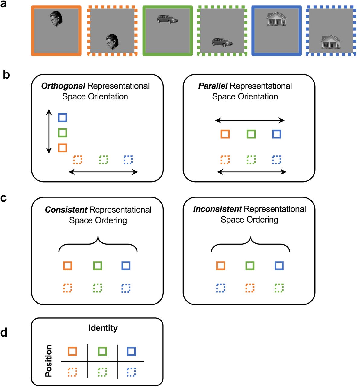
The representation of a set of objects across a visual transformation (e.g., at different positions of a visual scene) may be characterized by the orientation of these objects in the representational space and the consistency of the object representational structure (i.e., the ordering of these objects with respect to each other) across the transformation (see Figure 1 for an illustration). While it is possible to have non-parallel and consistent representations as well as parallel and non-consistent representations, to achieve untangled and tolerant visual object representations in high-level vision (DiCarlo and Cox, 2007), and allow representations to generalize across transformations (e.g., different positions), the orientation of the visual representational space for each transformation needs to be parallel to each other, and the consistency of the object representational structure needs to be preserved across transformations.

An illustration of the possible representational space structures for representing three objects across two positions. a. Three example objects shown in two different positions. b. Representational space orientation. The orientation of the representational space for each position may vary, from being orthogonal (left) to parallel (right). c. Representational space consistency. The ordering of objects with respect to each other at different positions may vary, from being consistent (left) to inconsistent (right). d. Transformation-tolerant object representation. At high-level vision, to achieve tolerance and allow object representations formed at one position to generalize to another position, the orientation of the visual representational space for each position needs to be parallel to each other, and the consistency of the object representational structure needs to be preserved across the position change.
While a parallel orientation and a high consistency are both necessary in achieving transformation-tolerant visual object representation in high-level vision, previous theoretical conjectures and experimental studies of object representation at the neuronal population level have not explicitly separated these two features and their unique contributions to tolerance. Specifically, past neurophysiological and fMRI studies have relied on cross-decoding measures (using a linear decoder) to evaluate the existence of tolerance at the neuronal population level (e.g., Hung et al., 2005; Rust & DiCarlo, 2010; Cichy et al., 2011; Vaziri-Pashkam & Xu, 2019; Vaziri-Pashkam et al., 2019). Such a cross-decoding approach is not sensitive to changes in the relative positions of the objects in the representational space, so long as the representations are still on the correct side of the decision boundary. Consequently, cross-decoding does not provide an accurate measure to changes in the representational space after transformation. Moreover, when there is a cross-decoding drop, it is unclear what is behind this drop: it could be caused by a change in the representational space orientation, a change to the representational consistency, or both.
Using position change as an example, because receptive field sizes are small in early visual areas, distinctive neuronal populations may represent objects at the top and bottom positions, resulting in an orthogonal orientation of these objects in the representational space (Figure 1). However, as receptive field sizes increase along the ventral visual pathway, the same neuronal population may represent the objects at both positions, resulting in a more parallel orientation of these objects in the representational space. Thus, with a broadening of neuronal tuning properties for nonidentity features such as position and size, the orientations of the representational space for objects under different states of a transformation become more parallel to each other in high-level vision.
Meanwhile, neurons in macaque IT cortex have been shown to maintain its relative selectivity (rank-order) for different objects across transformations even though the absolute neuronal responses might rescale with each state of a transformation (Schwartz et al., 1983; Tovee et al., 1994; Ito et al., 1995; DiCarlo & Manusell, 2003; Brincat & Connor, 2004; DiCarlo and Cox, 2007; Li et al., 2009; Murty & Arun, 2017). Such a neuronal response profile predicts that, at the population level, representational consistency across transformation would be present at high-level vision, with objects and categories arranged in similar order across an identity-preserving image transformation (Figure 1). This signature of tolerance at the population level, however, has never been directly tested. The first goal of the present study is therefore to document, using fMRI in the human brain, the existence of representational consistency across transformation at high-level vision and how it may emerge over the course of visual processing from lower to higher human visual areas.
Recent hierarchical convolutional neural networks (CNNs) have achieved human-like object categorization performance and are able to identify objects across a variety of identity preserving (sometimes quite challenging) image transformations (Yamins & Dicarlo, 2016; Kheradpisheh et al., 2016; Rajalingham, et al., 2018; Kriegeskorte, 2015; Serre, 2019). This has led to the thinking that CNNs likely form transformation-tolerant object representations in their final stages of visual processing similar to those seen in the primate brain (Hong et al., 2016; Yamins & Dicarlo, 2016; Tacchetti et al., 2018). CNNs incorporate the known architectures of the primate early visual areas and then repeat this design motif multiple times. Although the detailed neural mechanisms governing high-level primate vision remain largely unknow, CNNs’ success in object categorization under image transformations has generated the excitement that perhaps the algorithms essential to high-level primate vision would automatically emerge in CNNs to provide us with a shortcut to understand and model high-level vision. While CNNs are capable of associating the same label to an object undergoing different transformations, CNNs could succeed by simply grouping all instances of an object encountered during training under the same label without necessarily forming transformation-tolerant object representations like those found in high-level primate vision. Indeed, CNNs can achieve a near perfect classification accuracy even when image labels were randomly shuffled (Zhang et al. 2016), demonstrating their ability to memorize associations between images and random class labels. While this is one way to solve the invariance problem, this type of representation requires a large number of training data and has a limited ability to generalize to objects not included in training. Coincidentally, these two limitations have been argued to be the two major drawbacks associated with the current CNNs (Serre, 2019), raising the possibility that current CNNs may not actually form brain-like transformation-tolerant object representations in their final stages of visual processing. A second goal of the present study is therefore to document whether consistency across transformation develops in a similar manner in CNNs trained for object recognition as it does in the human brain, informing us the degree to which visual representation is similar between the human brain and CNNs.
To accomplish our goals, we took take advantage of existing human fMRI data sets and test object representational structure consistency across changes in position and size in the human ventral visual processing hierarchy. To increase signal to noise ratio (SNR), we examine the averaged response from multiple exemplars of an object category rather than the response of a single exemplar. The results from the human brain are then compared with those from 14 different CNNs trained to perform object categorization with varying architecture, depth and the presence/absence of recurrent processing. We find that while consistency across transformation increases over the course of visual processing across changes in position and size in human ventral visual regions, this is not found in CNNs trained for object categorization. If anything, consistency decreases in CNNs over the course of visual processing. CNNs thus do not appear to form the same kind of transformation-tolerant object representational structure as the human brain does.
Results
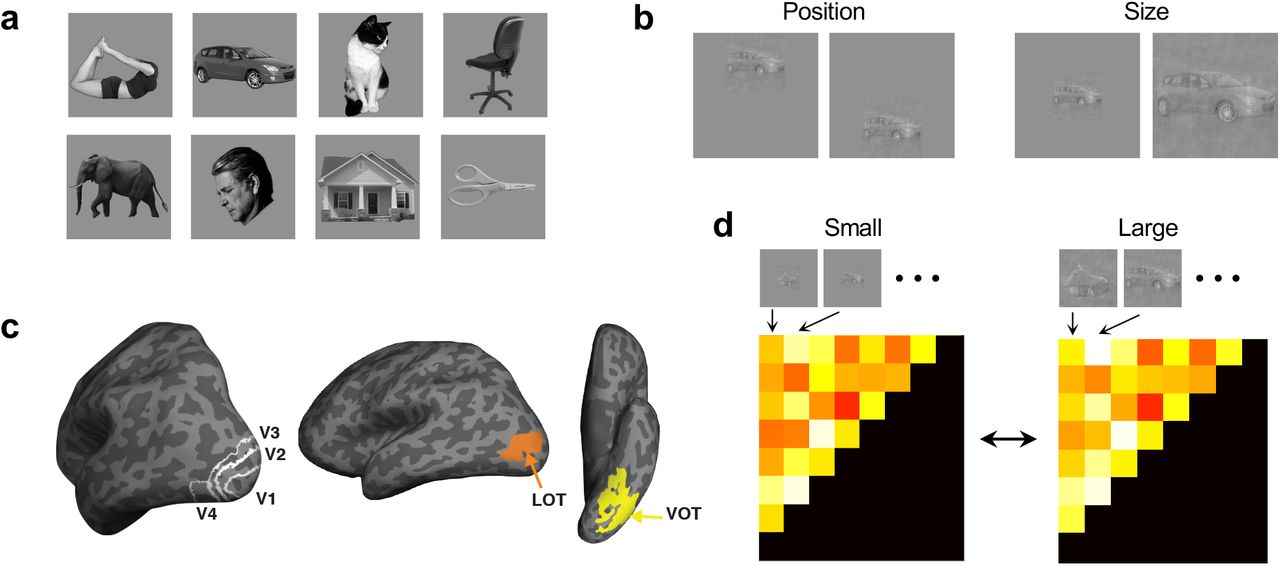
In two fMRI experiments, human participants viewed blocks of sequentially presented object images. Each image block contained different exemplars from the same object category. A total of eight real-world object categories were used, including bodies, cars, cats, chairs, elephants, faces, houses, and scissors (Vaziri-Pashkam & Xu, 2019; see Figure 2a). These object images were shown in two types of transformations: position (top vs bottom) and size (small vs large) (Figure 2b). To ensure that object identity representation in lower brain regions would reflect the representation of identity and not low-level differences among the images of the different categories, both experiments used controlled images with the spectrum, histogram, and intensity of the images normalized and equalized across the different categories (Willenbockel et al., 2010).

Stimuli used, brain regions examined, and the analysis applied in the study. a. The eight real-world object categories used with an example image shown for each category. Ten different exemplars varying in identity, viewpoint/orientation and pose/expression (for body, cat, elephant, face and scissor only) are shown for each category. b. Example images of the two types of nonidentity transformations examined: position (top vs bottom) and size (small vs large). To ensure that object identity representation in lower brain regions would reflect the representation of identity and not low-level differences among the images of the different categories, both experiments used controlled images with the spectrum, histogram, and intensity of the images normalized and equalized across the different category. c. The brain regions examined. They include topographically defined early visual areas V1 to V4 and functionally defined higher object processing regions LOT and VOT. d. Measuring representational space consistency across transformation (using size transformation as an example). For a given brain region or a sampled CNN layer, a representational dissimilarity matrix is first constructed by computing all pairwise Euclidean distances of fMRI response patterns or CNN output for all the object categories in one state of the transformation. The off-diagonal elements of this matrix are then used to construct a representational dissimilarity vector. The dissimilarity vectors from two states of a transformation are correlated to evaluate representational space consistency across transformation, with high correlation indicating a high consistency. a and c are reproduced from Xu and Vaziri-Pashkam (in press) with permission.
We examined fMRI responses from independently defined human early visual areas V1 to V4 and higher visual object processing regions LOT and VOT (Figure 2c). Reponses in LOT and VOT have been shown to correlate with successful visual object detection and identification (Grill-Spector et al. 2000; Williams et al., 2007) and their lesions have been linked to visual object agnosia (Goodale et al.,1991; Farah, 2004). These two regions have been argued to be the homologue of the macaque IT (Orban et al., 2004). For a given brain region, fMRI response patterns were extracted for each category for each type of transformations. Within each state of a given transformation (e.g., the upper position), we calculated pairwise Euclidean distances of the z-normalized fMRI response patterns for all the object categories to construct a category representational dissimilarity matrix (RDM, Kriegeskorte & Kievit, 2013, see Figure 2d; see Methods). We then correlated these RDMs between the two states of each transformation using Spearman rank correlation. To account for region-specific noise and ensure valid comparisons across brain regions, these correlations were corrected by the reliability of each brain region using a split-half measure before the results were compared across brain regions (see Methods).
For both position and size transformations, despite high RDM correlation across the two states of each transformation at the image pixel level due to the uniformity of the image pixel space (see Supplementary Results), RDM correlations of brain responses across the two states of each transformation were low at lower visual regions and gradually increased from lower to higher visual regions. Specifically, the linear correlation coefficients between the RDM correlations and the rank order of the brain regions, calculated within each participant and then averaged across participants, were .40 and .61, respectively for position and size, and both were significantly greater than 0, t(6) = 2.42, p = 0.026 for position, and t(6) = 4.11, p = 0.003 for size; all t-tests were one-tailed as the effects were tested for a specific direction). Additionally, correlations were higher between the average of LOT and VOT than the average of V1 to V3 for both position and size (t(6) = 2.59, p = 0.021 for position; and t(6) = 3.41, p = for size; the difference between LOT and VOT and those among V1 to V3 were not significant, all Fs < 1.31, ps > .29; see Figure 3a). Thus, for both position and size transformation, object representational consistency across transformation increased from lower to higher ventral visual regions. We noted that error bars for RDM correlations tended to be bigger in earlier than later visual areas. This was not due to a lower reliability of the data in early visual areas, but rather a consequence of object representations becoming more distinctive in higher than lower visual areas (see Supplementary Results). These results remain the same whether z-normalized Euclidean distance measure or correlation measure was used to construct the initial category dissimilarity matrix, and remained qualitatively similar even when Pearson correlation, rather than Spearman rank correlation, was applied (see Figure 3 - figure supplement 2).

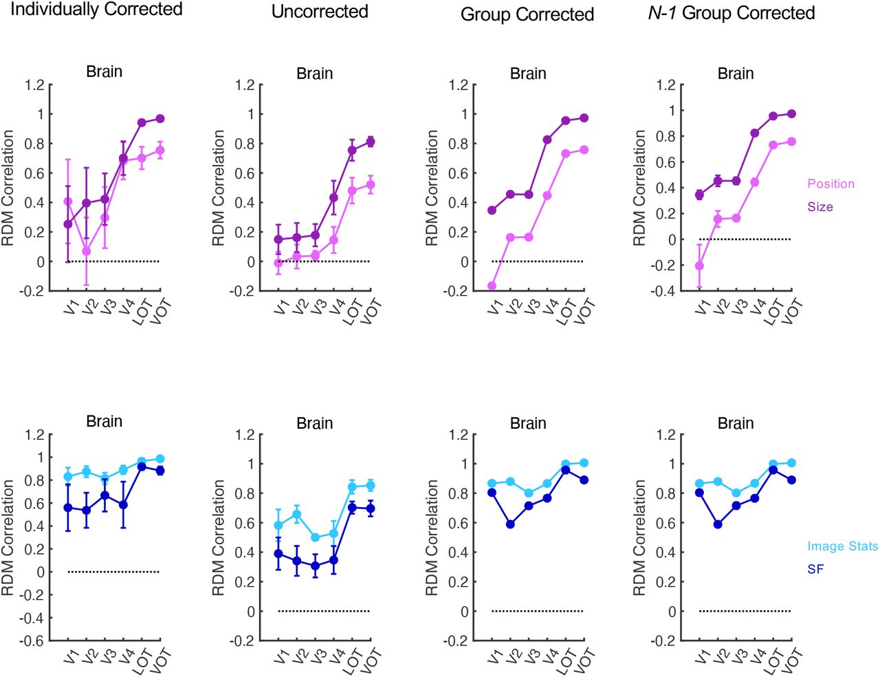
Evaluating representational space consistency across the four types of transformations in the human brain with different reliability correction method. Left most column, Individually Corrected. Here reliability is corrected within each participant before the results are averaged. These results are identical to those shown in Figure 3 and Figure 3 - figure supplement 5. These results are included here for comparison purposes. Second to left column, Uncorrected. Here no reliability correction is applied. Second to right column, Group Corrected. Here both correlation and reliability measures are first averaged across all participants. Reliability correction is then applied to these averaged values. Rightmost column, N-1 Group Corrected. Here group corrected correlations from N-1 participants are computed first and then averaged across all N iterations. Error bars represent standard errors of the means.

Evaluating representational space consistency across position and size changes in the human ventral visual pathway and 14 different CNNs with different analysis methods. a. Results from using Z-normalized Euclidean distances to construct the RDM within each state of a transformation and Spearman rank correlation to measure consistency across the transformation. These are the same results as those shown on Figure 3 and are included here for comparison purposes. b. Results from using Z-normalized Euclidean distances to construct the RDM within each state of a transformation and Pearson correlation to measure consistency across the transformation. c. Results from using correlations to construct the RDM within each state of a transformation and Spearman rank correlation to measure consistency across the transformation. All brain results are corrected by the reliability of each region. Very similar results were obtained from these different types of measures. Error bars represent standard errors of the means.

Evaluating representational space consistency in the human ventral visual pathway and 14 different CNNs across position and size changes. a. Representational space consistency for human ventral brain regions and CNNs. Results from the brain are corrected by the reliability of each region (see Methods). b. Response profile correlation between the brain and each CNN plotted against the upper and lower bounds of the noise ceiling of the brain responses. While representational consistency across position and size changes increases from lower to higher visual regions in the human brain, it decreases from lower to higher CNN layers, with all CNN response profiles showing a negative correlation with that of the brain. Error bars represent standard errors of the means.
We next examined whether CNNs exhibit a similar pattern in RDM correlation across the two states of each transformation from lower to higher layers. The 14 CNNs we examined included both shallower networks, such as Alexnet, VGG16 and VGG 19, and deeper networks, such as Googlenet, Inception-v3, Resnet-50 and Resnet-101 (Table 1). We also included a recurrent network, Cornet-S, that has been shown to capture the recurrent processing in macaque IT cortex with a shallower structure and have been argued to be the current best model of the primate ventral visual processing regions (Kubilius et al., 2019; Kar et al., 2019). All CNNs were pretrained with ImageNet images (Deng et al., 2009). Following a previous study (O’Connor et al., 2018), we sampled from 6 to 11 mostly pooling layers of each CNN (see Table 1 for the specific CNN layers sampled). We extracted the response from each sampled CNN layer for each exemplar of a category and then averaged the responses from the different exemplars within the same category to generate a category response for each state of a given transformation, similar to how an fMRI category response was extracted.
The CNNs and the layers examined in this study.
Despite differences in the exact architecture, depth, and presence/absence of recurrent processing, all CNNs exhibited overall similar trajectories over the course of visual processing for RDM correlation across both position and size transformations. Specifically, all CNNs showed overall high RDM correlation to position and size changes but with a downward trend from lower to higher layers (Figure 3a). Given that the earlier layers of CNNs are designed to be uniform across space and the heavy use of convolution in CNN architecture to capture translational invariance (LeCun, 1989), the high RDM correlation to both types of changes was expected; however, the downward trend across layers was not. This downward trend was much more prominent for size change, going from 1 to dropping below .8 from lower to higher layers across all the CNNs (in a number of CNNs the correlation dropped below .4), while the same correlation went from .2 to close to 1 from lower to higher brain regions (Figure 3a). Direct correlation of the overall response profiles over the course of visual processing using Spearman rank correlation revealed negative correlations between the brain and CNNs that were all significantly below the lower bound of the noise ceiling of the brain response across human participants (for position, ts > 2.62, ps < .020; for size, ts > 8.41, ps < .001; all t tests were one tailed as only testing for correlation below the lower bound of the noise ceiling was meaningful here; see Figure 3b). Thus, for position and size transformations, the object representational structure became less consistent from lower to higher CNN layers, the opposite of what was seen in the human brain. Despite CNNs’ success in classifying objects under identity preserving image transformations, how CNNs represent the relative similarity among the different objects appears to differ from that of the human brain. The built-in CNN architecture at the earlier layers likely gives it a boost in forming consistent object representational structures across transformation in early stages of processing compared to visual processing in the brain. However, such consistency is gradually lost during the course of processing in CNNs, such that the representations formed at final stages of CNN processing no longer appear to show high consistency across position and size transformations.
Although CNNs are believed to explicitly represent object shapes in the higher layers (Kriegeskorte, 2015; LeCun et al., 2015; Kubilius et al., 2016), emerging evidence suggests that CNNs may mostly use local texture patches to achieve successful object classification (Ballester & de Araújo, 2016, Gatys et al., 2017; Geirhos et al., 2019). However, when Resnet-50 is trained with stylized ImageNet images in which the original texture of every single image is replaced with the style of a randomly chosen painting, object classification performance significantly improves, relied more on shape than texture cues, and become more robust to noise and image distortions (Geirhos et al., 2019). When we compared the representations formed in Resnet-50 pretrained with ImageNet images with those from Resnet-50 pretrained with stylized ImageNet Images under three different training protocols (Geirhos et al., 2019), however, we found overall remarkably similar results in the RDM correlations across the two states of each transformation and all were different from what was seen in the human brain (Figure 3 - figure supplement 3). The inability of Resnet-50 to exhibit brain-like invariance in object representational structure across transformations suggests that there are likely fundamental differences between the two that cannot be easily overcome by this type of training.

Evaluating representational space consistency across position and size changes in the human ventral visual pathway and Resnet-50 under different training regimes. Resnet-50 is pretrained either with the original ImageNet images (RN50-IN), the stylized ImageNet Images (RN50-SIN), both the original and the stylized ImageNet Images (RN50-SININ), or both sets of images and then fine-tuned with the stylized ImageNet images (RN50- SININ-IN). The results do not appear to differ substantially across these different training regimes.
To further document potential processing differences between object categories and single objects, instead of object categories, we examined CNN representational structure for eight single object images (one from each of the 8 categories used in the fMRI experiments) undergoing the same two types of transformations. Additionally, we tested CNN representations for both the controlled images (as in the fMRI experiments) and the original images. We obtained virtually the same results. If anything, the decrease in consistency was more drastic for the single objects than for the object categories reported earlier (Figure 3 - figure supplement 4). A decrease, rather than an increase, in consistency across transformation over the course of CNN visual processing thus applies to both object categories and single objects.
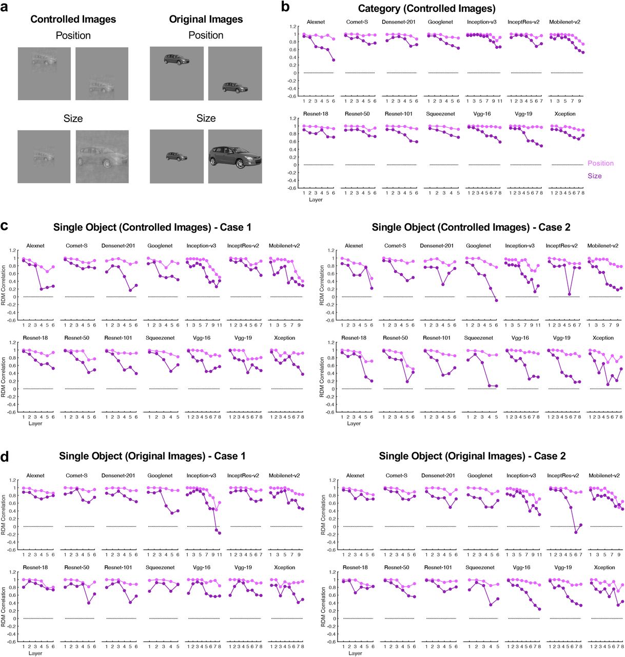
Evaluating representational space consistency across position and size changes for object categories and single objects in 14 different CNNs. a. Examples of the stimuli used. Both the controlled and the original images are used in this analysis. b. Representational space consistency for object categories using the controlled images. These are the same results as those reported on Figure 3 and are included here for comparison purposes. c. Representational space consistency for single objects using the controlled images. A single exemplar is chosen from each of the eight object categories for this analysis. This analysis is carried out twice, each involving a different exemplar from a given category. d. Representational space consistency for single objects using the original images. This analysis is also carried out twice, each involving a different exemplar from a given category. Similar results are obtained for object categories and single objects such that consistency generally decreases across position and size changes over the course of CNN processing. If anything, the decrease in consistency is more drastic for single objects than for object categories.
Besides position and size, we also tested two non-Euclidian transformations involving a change in image statistics (original vs controlled images) and the spatial frequency (SF) content of an image (high vs low SF) (see Supplementary Results). We again found an increase in representational consistency across these two transformations from lower to higher human visual regions, but not from lower to higher CNN layers (Figure 3 - figure supplement 5 to 8). Consistency in CNNs fluctuated across layers for these two types of transformations, showing a pattern that is different from the monotonic decreasing trend we saw in the human brain.
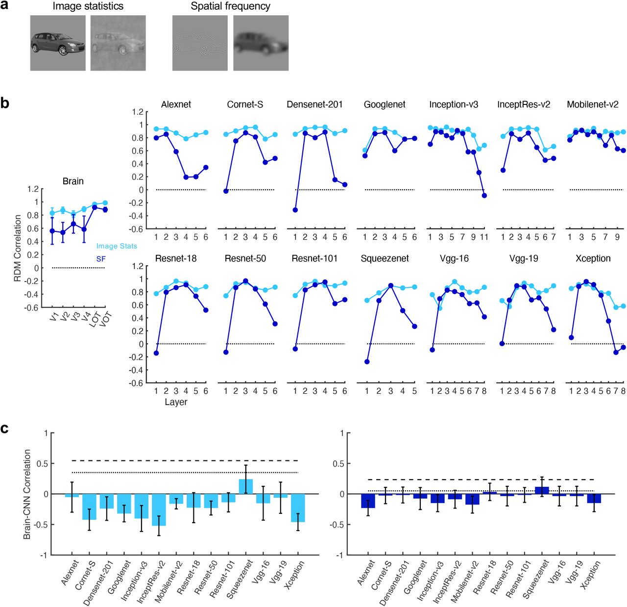
Evaluating representational space consistency in the human ventral visual pathway and 14 different CNNs across image stats and SF changes. a. Example images for the image stats change (original vs controlled) and SF change (high SF vs low SF). b. Representational space consistency across for human ventral brain regions and CNNs. Results from the brain are corrected by the reliability of each region (see Methods). c. Response profile correlation between the brain and each CNN plotted against the upper and lower bounds of the noise ceiling of the brain responses. While object representational structure becomes increasingly invariant from lower to higher levels of visual processing in the human brain, CNNs do not exhibit this response profile (see Supplementary Results for more details). Error bars represent standard errors of the means.

Evaluating representational space consistency across image Stats and SF changes in the human ventral visual pathway and 14 different CNNs with different analysis methods. a. Results from using Z-normalized Euclidean distances to construct the RDM within each state of a transformation and Spearman rank correlation to measure consistency across the transformation. These are the same results as those shown on Figure 3 - figure supplement 5 and are included here for comparison purposes. b. Results from using Z- normalized Euclidean distances to construct the RDM within each state of a transformation and Pearson correlation to measure consistency across the transformation. c. Results from using correlations to construct the RDM within each state of a transformation and Spearman rank correlation to measure consistency across the transformation. All brain results are corrected by the reliability of each region. Very similar results were obtained from these different types of measures. Error bars represent standard errors of the means.

Evaluating representational space consistency across image stats and SF changes in the human ventral visual pathway and Resnet-50 under different training regimes. Resnet-50 is pretrained either with the original ImageNet images (RN50-IN), the stylized ImageNet Images (RN50-SIN), both the original and the stylized ImageNet Images (RN50-SININ), or both sets of images and then fine-tuned with the stylized ImageNet images (RN50-SININ-IN). The results do not appear to differ substantially across these different training regimes.

Evaluating representational space consistency across image stats and SF changes for object categories and single objects in 14 different CNNs. a. Examples of the stimuli used. b. Representational space consistency for object categories. These are the same results as those reported on Figure 3 - figure supplement 5 and are included here for comparison purposes. c. Representational space consistency for single objects. A single exemplar is chosen from each of the eight object categories for this analysis. This analysis is carried out twice, each involving a different exemplar from a given category. Similar results are obtained for object categories and single objects with consistency across image stats and SF changes fluctuating over the course of CNN processing. If anything, the fluctuation in consistency is more drastic for the single objects than for the object categories.
Discussion
Forming transformation-tolerant object representations is essential for high-level primate vision. Although existing single cell neural recording findings predict the existence of highly consistent object representation across transformation in high-level vision, this key prediction has never been directly tested at the population level. Here we confirm this prediction using fMRI measures from the human brain. We show that high representational consistency across position and size changes indeed exists in human higher visual regions. Moreover, consistency is lower in early visual areas and increases as information ascends the human ventral visual processing pathway. We find similar results across image stats and SF transformations. Such a representation, however, is not found in 14 different CNNs trained for object categorization despite these networks capable to classifying objects under various transformations. For position and size changes, all CNNs show high representational consistency in earlier layers. Over the course of visual processing, however, consistency decreases in all CNNs tested, the opposite of what is seen in the human brain. For changes across image stats and SF, consistency in CNNs fluctuates across layers, again different from the monotonic decreasing trend we observe in the human brain (see Supplementary Results). Similar performance is observed for both shallow and deep CNNs (e.g., Alexnet vs Googlenet), and the recurrent CNN we tested, Cornet-S, does not outperform the other CNNs. Training a CNN with stylized images does not improve performance either. CNNs thus do not appear to maintain or increase representational consistency across transformations over the course of visual processing and form the same kind of transformation-tolerant object representational structure as the human brain does.
Given that CNNs are designed to be spatially uniform in the earlier layers, it is not surprising that lower CNN layers show high consistency in representation across position and size changes. However, this does not necessarily imply that lower CNN layers contain transformation-tolerant object representations for these two types of changes. As depicted in Figure 1, both a high consistency and a parallel representational orientation across a transformation are necessary to achieve tolerance. At the lower CNN layers, because the spatial receptive field size is small, largely nonoverlapping units may represent an object at different positions and sizes. This could result in the orientation of the objects in the representational space for different positions and sizes to be largely orthogonal (Figure 1b left), and a decreased ability for object representations to be generalized across positions and sizes using cross-decoding, even though consistency in representation is high.
It may be considered somewhat surprising that V1 does not appear to have a uniform representation across space. Because single neuron recording studies can only sample a limited number of neurons, the idea that information should be represented uniformly across the entire space in V1 has not been directly tested. The existence of hyper-columns in V1 does not require the distribution of features to be uniform across space. In fact, it is easier to have non-uniformity than maintain uniformity during development. Prior studies have also identified a number of systematic non-uniformity in representation in early visual areas, such as the cortical magnification factor (Daniel & Whitteridge, 1961), finer spatial and greater curvature representation in fovea than periphery (Srihasam, et al., 2014), radial bias in orientation representation (Sasaki, et al, 2006), and spatial field bias (Silson et al, 2018). Some of these factors could potentially contribute to the non-uniformity in feature representation in early visual areas as reported here. More research is needed to fully understand this result.
It may be argued that because fMRI is an indirect measure of neural activity at a coarse spatial resolution with its responses averaged over spatially contiguous neurons, it may not be valid to infer that differences in the representational structure of CNNs and human fMRI measures reflect actual differences in the internal representations of these two types of visual processing systems. This concern, however, has already been addressed by prior research and by our own work showing that there is a close correspondence in object representational structure between the fMRI measures obtained from the human brain and the unit responses obtained from CNNs when objects do not undergo transformation (i.e., when objects are shown in the same location at the same size). Using representational similarity analysis (RSA, Kriegeskorte & Kievit, 2013), Khaligh-Razavi and Kriegeskorte (2014) and Cichy et al. (2016) both report a close correspondence in representational structure (i.e., RDM) of lower and higher human visual areas to lower and higher CNN layers, respectively. Following this approach, using the same set of real-world object images and an identical experimental design as the present study, we also find a close correspondence in object representational structure between the human brain and the same 14 CNNs tested here, with lower visual areas showing better correlation with lower than higher CNN layers and the reverse being true for higher visual areas. This correspondence in brain-CNN representation is statistically significance in a majority of the CNNs examined here and replicates the results from Khaligh-Razavi and Kriegeskorte (2014) and Cichy et al. (2016). Remarkably, at the lower level of visual processing, our reported brain-CNN correlations in several CNNs are as good as brain-brain correlation among the human participants and these CNNs are able to capture 100% of the total explainable variance in human lower visual areas. Meanwhile, at higher levels of visual processing, CNNs can capture at most about 60% of total explainable variance in human higher visual areas. This is in agreement with the amount of variance CNNs can capture from macaque IT cortex in neurophysiology studies (e.g., Cadieu et al., 2014; Yamins et al., 2014; Kar et al. 2019; Bao et al., 2020). Thus, despite fMRI being an indirect measure of neural activity at a coarse spatial resolution, we are able to obtain highly similar results as those from neurophysiological studies. This provides validity and support for conducting the present investigation. Here we find that despite this close brain-CNN correspondence at lower levels of visual processing, none of the CNNs examined here exhibits the same representational consistency in the human brain at higher levels of visual processing.
Besides the RSA approach, using an encoding model approach, researchers have used linear transformation between fMRI voxels and CNN layer units to better align the two visual systems. Could the discrepancy we report here reflect a misalignment of brain and CNN features rather than some fundamental differences between the two? As mentioned earlier, we have shown that several CNNs examined are able to fully capture and account for 100% of the explainable variance in lower human visual areas for the exact same set of objects used here (Xu & Vaziri-Pashkam, 2021). There is thus already an excellent correspondence in lower-level visual processing between the brain and CNNs for the objects used here when transformation is held constant. No further linear transformation is therefore needed to align the fMRI voxels and CNN units. Supporting this, as mentioned earlier, both our RSA-based fMRI approach (Xu & Vaziri-Pashkam, 2021) and the encoding-model based neurophysiological approach (e.g., Cadieu et al., 2014; Yamins et al., 2014; Kar et al. 2019; Bao et al., 2020) find that CNNs can only account for about 60% of explainable variance in higher visual areas. Importantly, by examining representational consistency across transformation, our approach does not depend on the alignment of features between the brain and CNNs. But rather, by correlating the representational structure within each system after a transformation, we test if the two systems use a similar computational algorithm to achieve tolerance even if the precise features used for object representation may vary between the two. The discrepancy we report here thus suggests that the brain and CNNs likely differ in fundamental ways in how they achieve tolerance under transformation, rather than a superficial misalignment of visual features.
Although we examine object category responses averaged over multiple exemplars rather than responses to each object in an effort to increase SNR, previous research has shown similar category and exemplar response profiles in macaque IT and human lateral occipital cortex with more robust responses for categories than individual exemplars due to an increase in SNR (Hung et al., 2005; Cichy et al., 2011). Rajalingham, et al. (2018) recently report better behavior-CNN correspondence at the category but not at the individual exemplar level. Thus, comparing the representational structure at the category level, rather than at the exemplar level, should have increased our chance of finding a close brain-CNN correspondence. Importantly, our CNN results do not depend on the usage of object categories, as we show that a decreased consistency across transformations at higher levels of CNN visual processing applies to both object categories and single objects.
Our results add to the list of differences that have been reported between the brain and CNNs, such as CNNs’ ability to fully capture lower, but not higher, levels of visual representational structures of real-world objects as mentioned earlier and their inability to represent artificial objects like the human brain (Xu & Vaziri-Pashkam, 2021), differences in the representational strength of non-identity features across visual processing (Xu & Vaziri-Pashkam, in press), their ability to explain only about 60% of the response variance of macaque V4 and IT (Cadieu et al., 2014; Yamins et al., 2014; Kar et al. 2019; Bashivan et al., 2019; Bao et al., 2020), their usage of different features in object recognition (Ballester & de Araujo, 2016, Ulman et al., 2016; Gatys et al., 2017; Baker et al., 2018; Geirhos et al., 2019), and their susceptibility to the negative impact of adversarial images (Serre, 2019). While some of these discrepancies may be superficial (Firestone, 2020), our finding that representational consistency is not preserved in CNNs across transformation at higher level of visual processing indicate that CNNs likely uses a fundamentally different computational algorithm to solve the tolerance problem at high-level vision. With its vast computing power, CNNs likely associate different instances of an object via a brute force approach (i.e., by simply grouping all instances of an object encountered under the same object label) without increasingly preserving the relationships among the objects across transformations during the course of visual processing. Our findings are consistent with another study showing that while visual representations in humans exhibit tolerance to image changes across time, those from CNNs do not (Henaff et al., 2019). While some have regarded CNNs as the current best models of the primate visual system (Khaligh-Razavi & Kriegeskorte, 2014; Güçlü & van Gerven, 2015; Cichy et al., 2016; Eickenberg et al., 2017; Cichy & Kaiser, 2019; Kubilius et al., 2019), our results show that repeating the design motif of the primate early visual areas in CNN architecture may not be sufficient to automatically recover the algorithms used by primate high-level vision. Consequently, using the current state of CNNs as a shortcut to understand primate vision may be limited in helping us fully comprehend and model high-level primate vision.
The formation of transformation-tolerant object representations in the primate brain has been argued to be critical in facilitating information processing and learning by reducing the number of training examples needed while at the same time increasing the generalizability from the trained images to new instances of an object and a category (Tacchetti et al., 2018). Even if CNNs were to use a fundamentally different, but equally viable, computational algorithm to solve the object recognition problem compared to the primate brain, implementing a brain-like algorithm may nevertheless help them overcome the two major drawbacks currently associated with the CNNs: a requirement of large training examples and a limitation in generalizability to objects not included in training (Serre, 2019). That being said, making CNNs more brain like has its own practical advantages: as long as CNNs “see” the world differently from the human brain, they will make mistakes that are against human prediction and intuition. If CNNs are to aid or replace human performance, they need to capture the nature of human vision and then improve upon it. This will ensure the safety and reliability of the devices powered by CNNs, such as in self-driving cars, and, ultimately, our trust in using such an information processing system. Thus, in addition to benchmarking object recognition performance, it may be beneficial for future CNN architectures and/or training regimes to explicitly improve object representational consistency across transformation at higher levels of CNN visual processing. For example, preserving the similarity structure among the objects across transformation could be incorporated as a routine in CNN training. Doing so may push forward the next leap in model development and make CNNs not only better models for object recognition but also better models of the primate brain.
Materials and Methods
fMRI Experimental Details
Details of the fMRI experiments have been described in a previously published study (Vaziri-Pashkam & Xu, 2019). They are summarized here for the readers’ convenience.
Seven healthy human participants with normal or corrected to normal visual acuity, all right-handed, and aged between 18-35 took part in both the position and size experiments. All participants gave their informed consent prior to the experiment and received payment for their participation. The experiment was approved by the Committee on the Use of Human Subjects at Harvard University. Each experiment was performed in a separate session lasting between 1.5 and 2 hours. Each participant also completed two additional sessions for topographic mapping and functional localizers. MRI data were collected using a Siemens MAGNETOM Trio, A Tim System 3T scanner, with a 32-channel receiver array head coil. For all the fMRI scans, a T2*-weighted gradient echo pulse sequence with TR of 2 sec and voxel size of 3 mm x 3 mm x 3 mm was used. FMRI data were analyzed using FreeSurfer (surfer.nmr.mgh.harvard.edu), FsFast (Dale et al., 1999) and in-house MATLAB codes. FMRI data preprocessing included 3D motion correction, slice timing correction and linear and quadratic trend removal. Following standard practice, a general linear model was then applied to the fMRI data to extract beta weights as response estimates.
In the position experiment, we tested position tolerance and presented images either above or below the fixation (Figure 2b). We used cut-out grey-scaled images from eight real-world object categories (faces, bodies, houses, cats, elephants, cars, chairs, and scissors) and modified them to occupy roughly the same area on the screen (Figure 2a). For each object category, we selected ten exemplar images that varied in identity, pose and viewing angle to minimize the low-level similarities among them. Participants fixated at a central red dot throughout the experiment. Eye-movements were monitored in all the fMRI experiments to ensure proper fixation. During the experiment, blocks of images were shown. Each block contained a random sequential presentation of ten exemplars from the same object category shown either all above or all below the fixation. To equal low-level image differences among the different categories, controlled images were shown. Controlled images were generated by equalizing contrast, luminance and spatial frequency of the images across all the categories using the shine toolbox (Willenbockel et al., 2010, see Figure 2b). All images subtended 2.9° x 2.9° and were shown at 1.56° above the fixation in half of the 16 blocks and the same distance below the fixation in the other half of the blocks. Each image was presented for 200 msec followed by a 600 msec blank interval between the images. Participants detected a one-back repetition of the exact same image. This task engaged participants’ attention on the object shapes and ensured robust fMRI responses. Two image repetitions occurred randomly in each image block. Each experimental run contained 16 blocks, one for each of the 8 categories in each of the two image positions. The order of the eight object categories and the two positions were counterbalanced across runs and participants. Each block lasted 8 secs and followed by an 8-sec fixation period. There was an additional 8-sec fixation period at the beginning of the run. Each participant completed one scan session with 16 runs for this experiment, each lasting 4 mins 24 secs.
In the size experiment, we tested size tolerance and presented images either in a large size (5.77° x 5.77°) or small size (2.31° x 2.31°) centered at fixation (Figure 2b). As in the position experiment, controlled images were used here. Half of the 16 blocks contained small images and the other half, large images. Other details of the experiment were identical to that of the position experiment.
We examined responses from independent localized early visual areas V1 to V4 and higher visual processing regions LOT and VOT (Figure 2c). V1 to V4 were mapped with flashing checkerboards using standard techniques (Sereno et al., 1995). Following the detailed procedures described in Swisher et al. (2007) and by examining phase reversals in the polar angle maps, we identified areas V1 to V4 in the occipital cortex of each participant (see also Bettencourt & Xu, 2016) (Figure 2c). To identify LOT and VOT, following Kourtzi and Kanwisher (2000), participants viewed blocks of face, scene, object and scrambled object images. These two regions were then defined as a cluster of continuous voxels in the lateral and ventral occipital cortex, respectively, that responded more to the original than to the scrambled object images. LOT and VOT loosely correspond to the location of LO and pFs (Malach et al., 1995; Grill-Spector et al.,1998; Kourtzi & Kanwisher, 2000) but extend further into the temporal cortex in an effort to include as many object-selective voxels as possible in occipito-temporal regions.
To generate the fMRI response pattern for each ROI in a given run, we first convolved an 8-second stimulus presentation boxcar (corresponding to the length of each image block) with a hemodynamic response function to each condition; we then conducted a general linear model analysis to extract the beta weight for each condition in each voxel of that ROI. These voxel beta weights were used as the fMRI response pattern for that condition in that run. Following Tarhan and Konkle (2020), we selected the top 75 most reliable voxels in each ROI for further analyses. This was done by splitting the data into odd and even halves, averaging the data across the runs within each half, correlating the beta weights from all the conditions between the two halves for each voxel, and then selecting the top 75 voxels showing the highest correlation. This is akin to including the best units in monkey neurophysiological studies. For example, Cadieu et al. (2014) only selected a small subset of all recorded single units for their brain-CNN analysis. We obtained the fMRI response pattern for each condition from the 75 most reliable voxels in each ROI of each run. We then averaged the fMRI response patterns within each half of the runs and applied z-normalization to the averaged pattern for each condition in each ROI to remove amplitude differences between conditions and ROIs before further analyses were carried out (see more below).
Following previous studies, a vector in the neural space representing an object category in a given transformation state was obtained by vectorizing the z-normalized fMRI response pattern for that category in that state. The dimensionality of the vector was determined by the number of voxels included in each brain region (which was fixed to 75 most selective voxels). Euclidean distance between the end points of a pair of vectors was then calculated as the measure of similarity between these two vectors.
CNN details
We included 14 CNNs in our analyses (see Table 1). They included both shallower networks, such as Alexnet, VGG16 and VGG 19, and deeper networks, such as Googlenet, Inception-v3, Resnet-50 and Resnet-101. We also included a recurrent network, Cornet-S, that has been shown to capture the recurrent processing in macaque IT cortex with a shallower structure (Kubilius et al., 2019; Kar et al., 2019). This CNN has been recently argued to be the current best model of the primate ventral visual processing regions (Kar et al., 2019). All the CNNs used were trained with ImageNet images (Deng et al., 2009).
To understand how the specific training images would impact CNN representations, besides CNNs trained with ImageNet images, we also examined Resnet-50 trained with stylized ImageNet images (Geirhos et al., 2019). We examined the representations formed in Resnet-50 pretrained with three different procedures (Geirhos et al., 2019): trained only with the stylized ImageNet Images (RN50-SIN), trained with both the original and the stylized ImageNet Images (RN50-SININ), and trained with both sets of images and then fine-tuned with the stylized ImageNet images (RN50-SININ-IN).
Following O’Connor et al. (2018), we sampled between 6 and 11 mostly pooling and FC layers of each CNN (see Table 1 for the specific CNN layers sampled). Pooling layers were selected because they typically mark the end of processing for a block of layers before information is pooled and passed on to the next block of layers. When there were no obvious pooling layers present, the last layer of a block was chosen. For a given CNN layer, we extracted the CNN layer output for each object image in a given condition, averaged the output from all images in a given category for that condition, and then z-normalized the responses to generate the CNN layer response pattern for that object category in that condition (similar to how fMRI category responses were extracted). As with the fMRI responses, a vector in the CNN space representing an object category in a given transformation state was obtained by vectorizing the z-normalized CNN layer output pattern for that category in that state. The length of the vector was determined by the number of units in a CNN layer. Euclidean distance between a pair of vectors was then calculated as the measure of similarity between these two vectors.
Cornet-S and the different versions of Resnet-50 were implemented in Python. All other CNNs were implemented in Matlab. No averaging of space and feature was done for the CNN output. Output from all CNNs were analyzed and compared with brain responses using Matlab.
Comparing the representational structures between two states of a transformation in the brain and CNNs
Due to differences in measurement noise across the different brain regions, even if the representational structures were identical for the two states of a given transformation, the correlation between the two could vary across brain regions. To account for this potential variability across brain regions, we used a split-half approach by splitting the data into odd and even halves and averaging the data within each half (see also Xu & Vaziri-Pashkam, in press). To determine the extent to which object category representations were similar between the two states of each transformation in a brain region, within each half of the data, we first obtained the category dissimilarity vector for each of the two states of a given transformation. This was done by computing all pairwise Euclidean distances for the object categories sharing the same state of a transformation and then taking the off-diagonal values of this representation dissimilarity matrix (RDM) as the category dissimilarity vector. We then correlated the category dissimilarity vectors across the two states of a given transformation across the two halves of the data using Spearman rank correlation and took the average across both directions of the transformation as the raw RDM correlation (e.g., correlating odd run upper position with even run lower position and vice versa, and then taking the average of these two correlations). We calculated the reliability of RDM correlation by correlating the category dissimilarity vectors within the same state of a given transformation across the two halves of the data using Spearman rank correlation and took the average of both state of a given transformation as the reliability measure (e.g., correlating odd run upper position with even run upper position and correlating odd run lower position with even run lower position, and then taking the average of these two correlations). The final corrected RDM correlation was computed as the raw RDM correlation divided by the corresponding reliability measure. This was done separately for each ROI of each participant. In several participants the absolute value of the reliability measure was lower than that of the raw RDM correlation, yielding the corrected RDM correlation to be outside the range of [-1, 1]. Since correlation should not exceed the range of [-1, 1], any values exceeding the range were replaced by the closest boundary value (1 or -1). Without such a correction we obtained very similar line plots as those shown in Figure 3, but with a few large error bars due to a few excessively large values (greater than 10) obtained during the RDM normalization process. This only occurred for the early visual areas for the position manipulation, likely due to the small size of the visual stimuli used and consequently nosier neural measures obtained. The actual values would likely be lower than 1 (based on the mean of the other participants). In further analysis, instead of computing a normalized value for each participant, to deal with measurement noise more effectively, we averaged all values across participants first before computing a normalized value. Specifically, we averaged all the correlations of the same condition across odd and even runs across participants to compute a group average reliability score. We then averaged across participants the correlations of a pair of different conditions across odd and even runs to compute a group averaged correlation value for that pair. This correlation was then normalized by dividing its value by the group average reliability score. To derive error bars to better estimate the variance in these results, instead of averaging across all the participants in an experiment, we also averaged across n-1 participants at a time and then averaged the results. These results are shown in Figure 3 - figure supplement 1. These results replicated our individual participant normalized results, with low values in earlier regions and high values in higher regions.
To determine the extent to which object category representations were similar between the two states of each transformation in a CNN layer, from the CNN layer output, we first generated the object category dissimilarity vector for each state of a given transformation. We then correlated these vectors between the two states of the transformation using Spearman rank correlation. This was done for each sampled layer of each CNN.
To assess the similarity between the brain and CNN in their overall cross-transformation RDM correlation profile across regions/layers, we directly correlated the two using Spearman rank correlation. Before doing so, we first obtained the reliability of the RDM correlation profile across the group of human participants by calculating the lower and upper bounds of the noise ceiling following the procedure described by Nili et al. (2014). Specifically, the upper bound of the noise ceiling was established by taking the average of the Spearman correlation coefficients between each participant’s RDM correlation profile and the group average RDM correlation profile including all participants, whereas the lower bound of the noise ceiling was established by taking the average of the Spearman correlation coefficients between each participant’s RDM correlation profile and the group average RDM correlation profile excluding that participant. To evaluate the similarity in RDM correlation profile between the brain and a given CNN, we obtained the Spearman correlation coefficient between the CNN and each human participant and tested these values against the lower bound of the noise ceiling obtained earlier using a one-tailed t test. When the number of layers sampled in a CNN did not match the number of brain regions tested, bilinear interpolation was used to down sample the CNN profile to match with that of the brain. This allowed us to preserve the overall response profile of the CNN while still being able to carry out our correlation analysis. One-tailed t tests were used here as only testing values below the lower bound of the noise ceiling was meaningful here. If a CNN was able to fully capture the RDM correlation profile of the human brain, then its RDM correlation profile with the brain should be no different or exceed the lower bound of the noise ceiling.
Author contributions
The fMRI data used here were from two prior publications (Vaziri-Pashkam & Xu, 2019; Vaziri-Pashkam et al., 2019), with MV-P and YX designing the fMRI experiments and MV-P collecting and analyzing the fMRI data. YX conceptualized the present study and performed all the analyses reported here. YX wrote the manuscript with comments from MV-P.
Supplementary Results
Understanding the Error Bars for RDM Correlation
Error bars for RDM correlations tend to be bigger in earlier than later visual areas. This is not due to a lower reliability of the data in early visual areas: when we performed a split-half reliability measure on the actual fMRI response patterns (i.e., correlating the response pattern for each object category across odd and even halves of the runs and then average across categories and participants), we obtained > .90 correlation for all early visual areas. Instead, we believe this is a result of object representations becoming more distinctive from lower to higher visual areas (see Xu & Vaziri-Pashkam, in press, for a detailed documentation of this effect for the same data set). Consequently, even if the amount of noise were the same across brain regions, it would distort the representation structure more in earlier than in later visual areas, resulting in larger variance in RDM correlation in earlier areas.
Representational Consistency at Image Pixel Level
To benchmark the representational space correlation for the raw images, using pixel intensity as the input value, we vectorized the pixels for each image and then averaged all image vectors for a given category under one state of a given transformation to generate a category vector (similar to how fMRI responses and CNN layer responses were generated for a given category). We correlated the different category vectors to generate an RDM for each value of a transformation and then correlated the RDMs between the two values of that transformation as we did before to assess the consistency in the representational space across a given transformation.
Image pixel level RDM correlations between the two values of position, size, image stats and SF transformations were 1.00, .92, .13 and -.33, respectively. The high RDM correlations at the image pixel level for position and size transformation are the result of the uniformity of the image space. High RDM correlation at the image pixel level, however, did not directly translate into high RDM correlation at the early CNN layers: for image stats transformation, the RDM correlation was very low at the image pixel level but quite high (>.5) in CNN early layers. Likewise, high RDM correlation at the image pixel level did not directly correspond to high RDM correlation at the early visual regions: for both position and size, the RDM correlations were very high at the image pixel level but relatively low (<.5) in early visual areas.
Representational Consistency for Image Stats and SF Transformations
Besides examining the two Euclidian transformation involving position and size, we also tested two non-Euclidian transformations involving a change in image statistics (original vs controlled images) and the spatial frequency (SF) content of an image (high vs low SF). Although object representation has been shown to be invariant to the cues defining the shape (e.g., luminance, motion, or texture contrast) in macaque IT and human LOT and VOT (Sary et al., 1993; Grill-Spector et al., 1998), and the fact that we could recognize a line-drawing of a car just as easily as we do with a photograph of a car (which is similar to a SF transformation), tolerance for these two non-Euclidean image transformations has never been directly tested.
Details of the human fMRI image stats and SF experiments have been described in two previously published studies (Vaziri-Pashkam & Xu, 2019 and Vaziri-Pashkam et al., 2019). They are summarized here for the readers’ convenience. Six and ten participants took part in the image stats and SF experiments, respectively. In the image stats experiment, we tested image stats tolerance and presented images at fixation either in the original unaltered format or in the controlled format (subtended 4.6° x 4.6°) (Figure 3 - figure supplement 5a left). Half of the 16 blocks contained original images and the other half, controlled images. Other details of the experiment were identical to that of position experiment. In the SF experiment, only six of the original eight object categories were included and they were faces, bodies, houses, elephants, cars, and chairs. Images were shown in 3 conditions: Full-SF, High-SF, and Low-SF (Figure 3 - figure supplement 5a right). In the Full-SF condition, the full spectrum images were shown without modification of the SF content. In the High-SF condition, images were high-pass filtered using an FIR filter with a cutoff frequency of 4.40 cycles per degree. In the Low-SF condition, the images were low-pass filtered using an FIR filter with a cutoff frequency of 0.62 cycles per degree. The DC component was restored after filtering so that the image backgrounds were equal in luminance. Each run contained 18 blocks, one for each of the category and SF condition combination. Each participant completed a single scan session containing 18 experimental runs, each lasting 5 minutes. Other details of the experiment design were identical to that the position experiment. Only the results from the High-SF, and Low-SF conditions were included in the present analysis.
Results from the human fMRI image stats and SF experiments were analyzed following the same procedure as described in Methods. We obtained similar results for these two types transformations as we did for the position and size transformations in the human brain. Specifically, RDM correlation across the two states of each transformation linearly increased from lower to higher visual regions (the averaged linear correlation coefficients across participants were .43 and .28, respectively for image stats and SF, and both were greater than 0, t(5) = 2.58, p = 0.025 for image stats, and t(9) = 1.93, p = 0.043 for SF). RDM correlation between the two states of each transformation was also significantly higher for the average of LOT and VOT than the average of V1 to V3 (t(5) = 3.17, p = 0.012 for image stats; and t(9) = 2.37, p = 0.021, for SF; the difference between LOT and VOT and those among V1 to V3 were not significant, all Fs < 2.11, ps > .20; see Figure 3 - figure supplement 5b). These results remain the same whether z-normalized Euclidean distance measure or correlation measure was used to construct the initial category dissimilarity matrix, and remained qualitatively similar even when Pearson correlation, rather than Spearman rank correlation, was applied (see Figure 3 - figure supplement 6). Thus across both the two types Euclidian transformations examined (i.e., position and size) and the two types of non-Euclidian transformations examined here (i.e., image stats and SF), object representational structure across transformations becomes increasingly invariant from lower to higher ventral visual regions.
As in the main study, we next examined whether CNNs exhibit a similar pattern in RDM correlation across the two states of image stats and SF transformation from lower to higher layers. Despite differences in the exact architecture, depth, and presence/absence of recurrent processing, all 14 CNNs exhibited overall similar trajectories for a given transformation. Specifically, RDM correlations fluctuated across the different CNN layers, more drastically for SF than image stats, and showed an inverted U-shape between lower and higher layers in a large number of CNNs (Figure 3 - figure supplement 5b), rather than an increase in RDM correlation from lower to higher layers. This response pattern again differed from the monotonic increase in RDM correlation from lower to higher brain regions.
For the image stats transformation, direct correlation of the response profiles (using Spearman rank correlation) revealed in 10 out of the 14 CNNs negative correlations between the brain and CNNs that were significantly below the lower bound of the noise ceiling of the brain response across human participants (ts > 2.34, ps < .033; Figure 3 - figure supplement 5c). Three of the four CNNs that did not show a significant effect showed a marginally significant effect (Alexnet, t(5) = 1.64, p = 0.081; VGG-16, t(5) = 1.82, p = .064; and VGG-19, t(5) = 1.62, p = .084). The effect was not significant for Squeezenet (t(5) = .47, p = .33). For SF transformation, direct correlation of the response profiles between the brain and CNN revealed few significant or marginally significant correlations that were below the lower bound of the noise ceiling of the brain responses across human participants (Alexnet, t(9) = 2.26, p = .025; Inception-v3, t(9) = 1.42, p = .094; Mobilenet-v2, t(9) = 1.63, p = .069; Xception, t(9) = 1.42, p = .094; all other CNNs, ts < .94, ps >.19; Figure 3 - figure supplement 5c). Note that the overall response profiles were flatter for image stats and SF transformations in the brain than for the position and size transformations. Additionally, reliability for SF was low (close to 0 for the lower bound of the noise ceiling) even though more participants were included in this experiment. Both of these two factors likely contributed to the overall weaker differentiation between the brain and CNN response profiles for these two types of transformation than for position and size. Although strong conclusions may not be drawn from the direct response profile correlations for the image stats and SF transformation, given that consistency in object representational structure steadily increased for these two transformation from lower to higher human visual regions but not from lower to higher CNN layers, there still appeared to be some divergence between the brain and CNNs in how they represent these two types of transformations.
Acknowledgement
We thank Martin Schrimpf for help implementing CORnet-S, JohnMark Tayler for extracting the features from the three Resnet-50 models trained with the stylized images, and Thomas O’Connell, Brian Scholl, JohnMark Taylor and Nick Turk-Brown for helpful discussions and feedback on the results. This research was supported by National Institute of Health Grants (1R01EY030854 and 1R01EY022355) to Y.X. MVP was supported in part by NIH Intramural Research Program ZIA MH002035.
References


