

Abstract
The clock and wavefront model is one of the most accepted models for explaining the embryonic process of somitogenesis. According to this model, somitogenesis is based upon the interaction between a genetic oscillator, known as segmentation clock, and a moving wavefront, which provides the positional information indicating where each pair of somites is formed. Recently, Cotterell et al. (2015) reported a conceptually different mathematical model for somitogenesis. The authors called it a progressive oscillatory reaction-diffusion (PORD) model. In this model, somitogenesis is driven by short-range interactions and the posterior movement of the front is a local, emergent phenomenon, which is not controlled by global positional information. With the PORD model, it was possible to explain some experimental observations that are incompatible with the clock and wavefront model. However the PORD model has the disadvantage of being quite sensitive to fluctuations. In this work, we propose a modified version of the PORD model in order to overcome this and others inconveniences. By means of numerical simulations and a numerical stability analysis, we demonstrate that the modified PORD model achieves the robustness characteristic of somitogenesis, when the effect of the wavefront is included.
1. Introduction
Somitogenesis, the process by which somites are formed, is an essential developmental stage in many species. Somites are bilaterally paired blocks of mesoderm cells that form along the anterior-posterior axis of the developing embryo in segmented animals (Maroto et al., 2012). In vertebrates, somites give rise to skeletal muscle, cartilage, tendons, endothelial cells, and dermis. Somites form with a strikingly regular periodicity, that is preserved among embryos of a single species. From this, and other reasons, scientists have been attracted to somitogenesis for decades. One of the earliest conceptual attempts to explain this regularity is the so-called clock and wavefront model, originally proposed by Cooke and Zeeman (1976). According to this model, somitogenesis occurs due to the interaction between: (i) autonomous oscillations of a network of genes and gene products, which causes presomitic-mesoderm cells to oscillate between a permissive and a non-permissive state, in a consistently (clock-like) timed fashion; and (ii) a wavefront (also known as determination front) of signaling that slowly progresses in an anterior-to-posterior direction. As the wavefront comes in contact with cells in the permissive state, they undergo a mesenchymal-epithelial transition, forming a somite boundary, and resetting the process for the next somite.
The clock and wavefront model gained relevance when the expression of several genes under the Notch, Wnt, and FGF pathways was discovered to oscillate cyclically, with the same period as that of somite formation (Palmeirim et al., 1997; Pourquié, 2001; Gibb et al., 2010; Pourquié, 2011). This, together with the existence of substances, like Wnt3a and FGF8, whose concentrations vary along the presomitic mesoderm in characteristic patterns that travel at constant velocity in an anterior to posterior direction, seemed to confirm the general assessments of the clock and wavefront model (Dubrulle et al., 2001; Gibb et al., 2010; Pourquié, 2011). As a matter of fact, this model has been very successful because it agrees with numerous experimental observations, and because much progress has been done in elucidating the segmentation-clock clockwork, and the way it interacts with the Wnt3a and FGF8 gradients. Despite its success, some experimental observations have been reported that are incompatible with the clock and wavefront paradigm. For instance, somites can form in the absence of Wnt or FGF gradients, albeit in a disorderly fashion (Naiche et al., 2011; Dias et al., 2014).
Recently, Cotterell et al. (2015) introduced a novel mathematical model for somitogenesis. Contrarily to the clock and wavefront model, in the model by Cotterell et al.—which the authors call a progressive oscillatory reaction-diffusion (PORD) system—somitogenesis is driven by short-range interactions. Hence, the posterior movement of the front is a local, emergent phenomenon, that is not controlled by global positional information. As shown by Cotterell et al., their PORD model is compatible with several important features of somitogenesis (like size regulation), that former reaction-diffusion models were unable to explain. Furthermore, the PORD model makes predictions regarding FGF-inhibition and tissue-cutting experiments that are more consistent with experimental observations than those of clock and wavefront models.
At the core of the Cotterell et al. model there is a gene regulatory motif schematically depicted in Fig. 1. In this network, a hypothetical gene codes for an activator protein (A), which enhances its own expression, as well as that of another gene that codes for a hypothetical repressor protein (R). In turn, the repressor protein down-regulates the gene coding for the activator, and is able to diffuse into the extracellular medium and affect neighboring cells. Cotterell et al. did not identify the network genes, but showed that in case it existed, the gene network in Fig. 1 can explain most of the experimental observations regarding somitogenesis. In particular, with the correct parameter values, such gene network can generate sustained oscillations, and when repressor diffusion is included, it gives rise to a stationary pattern of gene expression like that observed in somitogenesis, even in the absence of a FGF wavefront.

Schematic representation of the gene regulatory network introduced by (Cotterell et al., 2015) and studied in the present work. This network consists of two genes: an activator A and a repressor R. Solid lines ending in arrowheads (hammerheads) denote positive (negative) regulation. β represents external regulation of gene A via a wavefront substance. Dashed lines correspond to passive diffusion into the extracellular medium. The diffusion process depicted by the blue arrow was not originally included in the Cotterell et al. model, but is included in the modified model version studied in this work.
Even though the hypothetical genes in the Cotterell et al. model have not been identified, we find this model interesting for the following reasons: (i) as far as we have observed, it accounts for some important features of somitogenesis that traditional clock and wavefront models fail to explain; (ii) a gene network with a similar architecture as that of Fig. 1—albeit with a different dynamic behavior—has been invoked to explain oscillation arrest in somitogenesis (Santillán and Mackey, 2008; Zavala and Santillán, 2012); and finally, (iii) the architecture of the gene network in Fig. 1 is an ubiquitous motif in the intricate transcription-factor regulatory network of the genes under the Wnt, Notch and FGF pathways (Gibb et al., 2010; Zavala and Santillán, 2012).
In opposition to its multiple virtues, the Cotterell et al. model is quite sensitive to fluctuations. For instance, when random perturbations of initial conditions or intrinsic noise are present, a disordered pattern of gene expression arises. This behavior resembles what happens with PSM cells that are not under the influence of a wavefront, but contrasts with the observed robustness of somite formation under normal conditions. We hypothesize from the above discussion that, although a wavefront is not strictly necessary for the Cotterell et al. model to generate a gene expression pattern consistent with somitogenesis, the interaction with a wavefront is essential to explain the observed robustness of this phenomenon. The present work is aimed at testing this hypothesis, and discussing the corresponding biological implications.
The manuscript is organized as follows. In section 2 we develop an extension of the Cotterell et al. model, which is aimed at avoiding some of the former model inconveniences. In section 3 we define the parameter set where the dynamics of the non-diffusion system give place to a limit cycle family. In section 4 we explain the numerical methods used as well as the initial and boundary conditions. In section 5 we show results of the simulations for each one of the selected conditions. Finally, we discuss the relevance of the results obtained as well as the limitations of the model in section 6.
2. Mathematical Model
In this section, we introduce a modified version of the Cotterell et al. model. As the functions taken into account in the original model are unrealistic from a biochemical point of view, we propose key modifications, which consist in replacing the gene-expression regulatory functions and introducing a diffusion transport process for both activator and repressor protein concentrations.
Consider the gene network schematically represented in Fig. 1. Assume that the half life of mRNA molecules corresponding to genes A and R is much shorter than that of the corresponding proteins. Then, a quasi-stationary approximation can be made for the equations governing mRNA dynamics, which yields the following reaction-diffusion system for the concentration of proteins A and R:

 where αA and αR are the maximum possible rate of activator and repressor production; PA and PB are the probabilities that the promoters of genes A and R are active; degradation rate constants of each protein concentration are denoted by μA and μR, respectively; and DA and DR are the corresponding diffusion coefficients.
To take into account the roles of the activator and the repressor, PA(A, R) must be a monotonic increasing (decreasing) function of A (R), while PR(A) ought to be a monotonic increasing function of A. Indeed, Cotterell et al. (2015) proposed the following functions:

 where l1, l2, and l3 define the strengths of regulatory interactions between A and R, and β is the background regulatory input of A. To prevent negative values, Cotterell et al. introduced the function Φ(x) = x.H(x), where H(x) is the standard Heaviside function (H(x) = 1 for x ≥ 0 and H(x) = 0 for x < 0).
Even though the function PA(A, R) defined in (2a) fulfills the requirement of being a monotonic decreasing function of R and a monotonic increasing function of A, it shows features that are biologically challenging:
There is neither biological nor biochemical motivation for the introduction of function Φ.
Function Φ(x) is non smooth at the origin. This feature is unusual in biologically inspired mathe-matical models, and may cause unexpected complications while studying the dynamical system.
Since the term l2R appears with negative sign in the denominator of the argument of function Φ, in the right hand side of Eq. (2a), function PA(A, R) may be divergent for certain values of A and R.
In order to address the above discussed issues, we propose a slightly novel approach by substituting the promoter-activation probabilities in (2) with functions that are consistent with the assumptions that the activator and the repressor compete for the same binding site in the promoter region of gene A, and that both the activator and the repressor interact with their corresponding binding sites in the promoter regions of genes A and R in a cooperative fashion (Santillán, 2008). In so doing, we have

 where K1 denotes the half saturation constant for the binding reaction between the activator and the promoter of gene A; the Hill coefficient that accounts for a cooperative interaction between the activator and gene A promoter is given by n1; as in the original model, β is the background regulatory input of A; the half saturation constant and Hill coefficient of the interaction between the repressor and the promoter of gene A are represented by K2 and n2, respectively; and K3 and n3, equivalently, are the half saturation constant and Hill coefficient for the interaction between the activator and the promoter of gene R.
Notice that (1) along with (3) constitute a reaction-diffusion system for the gene expression network depicted in Fig. 1, which accounts for spatio-temporal interactions between these two protein concentrations.
Upon re-scaling position and time as x′ = x/L, y′ = y/L, z′ = z/L, and t′ = tμA and substituting the following dimensionless variables and parameters
 where L is a characteristic length on system (1)-(3), we obtain the reaction-diffusion system in a dimensionless form

 where ∇′ is the Laplacian with respect to (x′, y′, z′), and


To ease notation, we suppress symbol (·)′ from this point onward along the paper.
3. Parameter estimation
Since the genes here modeled are hypothetical, it is impossible to estimate the model parameter values from experimental data. Instead, we performed a bifurcation analysis of the system with no diffusion (da = dr = 0), employing a continuation method implemented in XPPAUT (Ermentrout, 1987). The results of this analysis are presented in Fig. A.1 of Appendix A. From this analysis, we determined the parameter intervals (see Table 1) for which the system shows sustained oscillations in the absence of diffusion, which is crucial to set the periodicity of somitogenesis. In our simulations, we consider parameter values in the middle of the intervals reported in Table 1. Following (Cotterell et al., 2015), we fixed n3 = μ = 1, and assumed that n = n1 = n2. After this, the only free parameters in the model are the diffusion coefficients.
Parameter intervals for which the system with no diffusion shows sustained stable oscillatory behavior.
4. Numerical methods
Under the supposition that the presomitic mesoderm (PSM) can be regarded as one-dimensional, we considered a single spacial dimension, x, with boundaries at x = 0 and x = 1. These boundaries set an observation window in the PSM, where x = 0 corresponds to the posterior extreme. To numerically solve system (4), we implemented a standard finite-difference three-point stencil and Euler’s algorithm in Julia; homogeneous Neumann boundary conditions were included:
 with, unless otherwise stated, the following initial conditions:

That is, the system is assumed to be initially homogeneous, except for a perturbation at the anterior extreme of the observation window.
We also performed stochastic simulations in which additive white noise was added to the system. For these simulations we substituted equations (4a) and (4b) by

 where
where  and
and  respectively denote the stationary values of a and r, cv is the coefficient of variation of the added white noise, and dW is a normally-distributed white noise term with mean zero and variance 1. To solve this system of stochastic partial differential equations we employed the Euler-Maruyama method, implemented in Julia.
5. Results
We started by reproducing the results in (Cotterell et al., 2015). To this end, we set da = 0, dr = 2.5 10−3, β = 0.5, and numerically solved the model equations as described in Section 4. The simulation results are shown in Fig. 2A. Observe that an oscillatory behavior gradually gives rise to a steady pattern consisting of alternated high and low gene-expression regions. Notice as well that the pattern formation dynamics start at the initial perturbation position, and propagate with constant speed. The initial perturbation is essential for the appearance of the pattern. If the system is initially homogeneous, the oscillatory behavior continues indefinitely—see Fig. 2B. On the other hand, when more than one initial perturbations are present, each one of them originates a pattern-formation wave, and when two such waves collide, they cancel out—see Fig. 2C. These results suggest that the transition from an oscillatory behavior to a steady pattern of gene expression is due to a diffusion driven instability interacting with a limit cycle. To verify this, we investigated the spatial stability of the dynamical system in (4) and (5) in Appendix A. We were able to confirm that the limit cycle is unstable with the current parameter values set; see Fig. A.3, panel (c), at κ2 = 0.
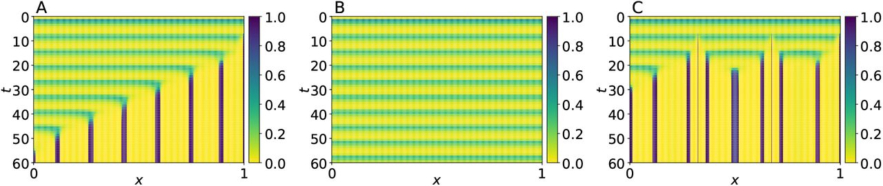
Spatio-temporal evolution of a from system (4), with boundary condition as in (5), for different initial conditions: (A) r(x, 0) = 0 for all x ∈ [0, 1], a(x, 0) = 0 for 0 ≤ x < 1, and a(1, t) = 0.05; (B) r(x, 0) = a(x, 0) = 0 for all x ∈ [0, 1]; (C) r(x, 0) = 0 and a(x, 0) = 0 for all x ∈ [0, 1] and a(x′, 0) = 0.05 at x′ = 0.325, 0.675, 0.9975. Parameter values were set as follows: k1 = 0.05, k2 = 0.01, k3 = 2, n = 3, β = 0.5, da = 0, and dr = 2.5 × 10⁻³.
The results described in the previous paragraph are consistent with the reported experimental observations that somites can form in the absence of a wavefront. As a matter of fact, they explain why somites form almost simultaneously and irregularly; in other words, any initial perturbation in the mesoderm tissue rapidly originates a somite boundary, and the emerging pattern formation wave almost immediately collides with neighboring waves. However, even though the wavefront is not strictly necessary for the formation of somites, there are several reports that confirm its importance (Sawada et al., 2001; Naiche et al., 2011). In particular, the regularity of somite formation has been demonstrated to be extremely robust to many different kinds of perturbations on both the mesoderm tissue and the differentiation wavefront, which is not explained by the current PORD model.
We hypothesize that somitogenesis robustness can be achieved via the interaction between the gene network and a wavefront. This wavefront is originated by substances, like FGF8 (in what follows we refer to FGF8 only, but the discussion applies to other substances as well, like Wnt3a), which are produced in the embryo tail bud and diffuse to the rest of the PSM. In consequence, FGF8 concentration decreases in the posterior to anterior direction. On the other hand, as the embryo grows, the tail bud recedes leaving PSM cells behind. Hence, the spatial FGF8 distribution moves in the anterior to posterior direction, like a wave-front, as time passes. In other words, we expect that a stable limit cycle emerges for large enough values of β (that accounts for the PSM interaction with the wavefront), which maintains an oscillatory gene expression despite perturbations, thus preventing somite formation close to the tail bud. Furthermore, if the limit cycle turns unstable below a given β threshold, any perturbation would lead to the formation of a somite at the PSM position where the threshold is reached. This dynamic behavior may explain why somites are formed in an irregular fashion in the absence of FGF8, and how a FGF8 wavefront robustly drives somitogenesis.
In Appendix, A we analyze the stability of the PDE system when depending of β and da parameters, and found that for a fixed value for da = 5 × 10⁻⁵ the system undergoes a bifurcation from a stable to an unstable limit cycle as the value of β decreases. To illustrate these findings, we present in Fig. 3 the results of two simulations: one in which the limit cycle is stable and another in which it is unstable. In Fig. 4 we present the results of two more runs where, instead of considering a constant value of β, we assume that it is given by


Spatio-temporal evolution of a from system (4), with boundary condition as in (5), for: (A) spatially stable with β = 0.5; (B) spatially unstable with β = 0.01. In both cases, the initial conditions for a were selected from random uniform distributions in the interval [0, 0.1], whereas we set r(x, 0) = 0 for all x ∈ [0, 1]. Parameter values were set as follows: k1 = 0.05, k2 = 0.01, k3 = 2, n = 3, da = 5 × 10⁻⁵ and dr = 2.5 × 10⁻³.

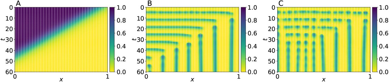
Spatio-temporal evolution of a from system (4) for β-wave speed as in (8), with boundary condition as in (5). (A) β-wave evolution and (B) somite-pattern formation for speed v = 0.02; (C) β-wave evolution and (D) somite-pattern formation for speed v = 0.04. Initial conditions for a consists of random uniform distributions in the interval [0, 0.1], whereas r(x, 0) = 0 for all x ∈ [0, 1]. Parameter values were set as follows: k1 = 0.05, k2 = 0.01, k3 = 2, n = 3, da = 5 × 10⁻⁵ and dr = 2.5 × 10⁻³.
Notice that this expression corresponds to a external regulation of gene A, which is a temporarily and spatially dependent profile that decays in a sigmoidal fashion in the posterior to anterior direction, and travels with speed v > 0 in the opposite direction. That is, it mimics the behavior of the FGF8 profile. For the simulations in Fig. 4 we set K = 0.9, n = 16 (these values were also employed for the simulation in Fig. 5), and considered two different speed values v = 0.02, and v = 0.04. Observe that, in both simulations, the pattern formation waves have the same periodicity, but the regions corresponding somites are larger for the faster wave. This result agrees with the experimental observation that somites are larger when the velocity of FGF8 profile is increased (Sawada et al., 2001).

Spatio-temporal evolution of A from system (7) for β-wave speed as in (8), with boundary condition as in (5): (A) β-wave evolution for speed v = 8 for somite-pattern formation with noise intensity (B) cv = 0.05 and (C) cv = 0.1. Initial conditions for A consists of random uniform distributions in the interval [0, 0.1], whereas R(x, 0) = 0 for all x ∈ [0, 1]. Parameter values were set as follows: k1 = 0.05, k2 = 0.01, k3 = 2, n = 3, da = 5 × 10⁻⁵ and dr = 2.5 × 10⁻³.
Finally, we performed simulations in which additive white noise was added to both variables (a and r), and confirmed the robustness of the system behavior to this kind of variability. As can be seen in Fig. 5, results of a typical simulation show that, when the noise coefficient of variation is cv = 0.05, somite formation proceeds in a very precise way, despite the relatively large fluctuations in the gene expression level. On the contrary, when cv = 0.1, although somites continue sequentially emerging, the periodicity of somitogenesis is lost, as well as the regularity of somite sizes.
To summarize, the results presented in the paragraphs above confirm the hypothesis that a PORD model (modified to include diffusion of both the repressor and the activator) undergoes a bifurcation from a stable to an unstable limit cycle, as a result of its interaction with the wavefront, and that this bifurcation is enough to explain the observed robustness of somitogenesis. To the best of our understanding, the modified PORD model has a couple of quintessential features: it explains why somitogenesis may occur in the absence of a wavefront and its inherent somites irregular prompting, and how the process achieves robustness as a consequence of the wavefront.
6. Concluding Remarks
We have studied a modified version of the somitogenesis PORD model originally introduced by Cotterell et al. (2015). The most important of the introduced modifications is the assumption that the activator protein can also diffuse, although with a much smaller diffusion coefficient than the repressor. With this modification, the model undergoes a bifurcation, from a stable to an unstable limit cycle, as the value of the parameter accounting for the background regulatory input of the activator decreases. From a biological perspective, the bifurcation just described allows the model to explain why somites can form in the absence of a wavefront (which traditional front and wavefront models failed to explain), reassesses the role of the wavefront as a conductor for somitogenesis, and makes the model behavior robust to random fluctuations; notice that the latter is one of the weak points of the original PORD model.
In the clock and wavefront models, there is a consensus that the oscillatory behavior is originated by a gene network with time-delayed negative feedback regulation (Monk, 2003; Lewis, 2003). This claim is supported by multiple experimental reports, which have elucidated some of the underlying regulatory mechanisms (Schröter et al., 2012). In contrast, the present and the Cotterell et al. (2015) models not only rely on a different gene network architecture to generate oscillations, but the genes in the network are hypothetical. From this perspective, the weight of experimental evidence seems to favor clock and wavefront models. Nonetheless, upon taking this into consideration, we believe that we have provided convincing evidence that reaction-diffusion and positional information (wavefront) mechanisms could work together in somitogenesis. Further investigating this possibility may allow a better understanding of such a fascinating phenomenon.
Acknowledgements
JP-H thanks CONACYT-México for granting him a doctoral scholarship. VFBM thanks the financial support by Asociación Mexicana de Cultura AC. MS acknowledges the financial support of CONACYT-México, grant INFRA-302610.
Appendix
Appendix A. Somite pattern-formation dynamical features
System (4), along with homogenous Neumann boundary conditions, gathers the essential ingredients of somite pattern-formation dynamics. Particularly, the kinetic terms consist of Hill functions, whose coefficients corresponding to a non-negative cooperative interaction. Thus, we assume that n3 = 1 and n1 = n2 = n ≥ 1 as well as μ = 1. Initially, we set da = dr = 0. In so doing, we get the purely kinetic system:
 where the field components are given by

This system steady states satisfy the relation g(a) = β, where


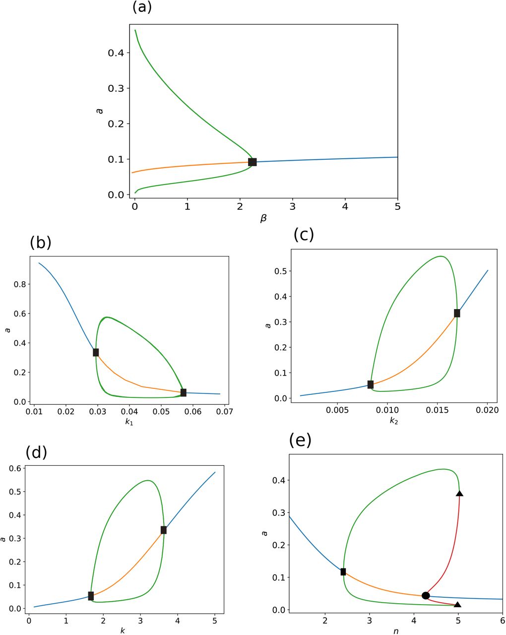
Bifurcation diagrams of system (A.1) for slowly varying: (a) background regulatory input of activator β, effective half-saturation parameters (b) k1, (c) k2 and (d) k3, and (e) Hill coefficient n. Blue (orange) solid lines correspond to stable (unstable) branches of steady states, and green (red) lines are stable (unstable) limit-cycle branches. Squares (filled circle) indicate supercritical (subcritical) Hopf bifurcations, and triangle is for indicating fold bifurcations. Other parameter set values are k1 = 0.05, k2 = 0.01, k3 = 2.0, n = 3.0, and β = 0.5, respectively.
From (A.2), notice that g(a) satisfies that: (i) g(0) = 0, and (ii) g(a) → +∞, when a → +∞. In consequence, there exists a* > 0 such that g(a*) = β > 0, which further implies that w* = (a*, r*) is a steady-state of system (A.1), with a* > 0 and r* > 0, since

In other words, the existence of at least one steady-state in the first quadrant is guaranteed. We can straightforwardly prove, from the Poincare-Bendixon theorem, that a limit-cycle family emerges as a result of this steady-state undergoing a Hopf bifurcation (HB). In order to disclose this implication, we performed a numerical continuation by using the algorithms implemented in XPPAUT (Ermentrout, 1987). The resulting bifurcation diagrams obtained by slowly varying each parameter of system (A.1) are depicted in Fig. A.1. Notice that the system undergoes HBs for all parameters values in Table 1. In Fig. A.1(a), a single HB for parameter β takes place, where periodic orbits vanish at the bifurcation point HB. This suggests that the lower the β-input value, the larger the amplitude and the longer the period of stable orbits for the homogeneous system; and that no periodic orbits occur for β ≫ 1, nonetheless. In contrast, as is shown in Figs. A.1(b)-(d), two supercritical HB points occur for parameters k1, k2 and k3, which determine a finite interval for each parameter wherein a family of periodic orbits exist. Interestingly, a bi-stability interval for parameter n is delimited by n-values where a subcritical HB and fold bifurcation (LP) points happen. That is, a branch consisting of unstable limit cycles emanates from the subcritical HB, which stabilizes at the LP points. Hence, stable steady-states coexist with stable limit-cycles for this interval, where the unstable periodic branch plays a critical role for initial states. This result, as is depicted in Fig. A.1(e), indicates that an on-and-off gene switch is present, which provides hysteretical features triggered by key values of the characteristic Hill coefficient. We may argue from this that the cooperativity in the gene regulatory network favors system robustness to parameter variations.
On the other hand, as has been discussed above, the external regulation of gene A is an essential ingredient of the somite pattern formation dynamics. Recall that this element is captured by β. In addition, the activator diffusion also plays a crucial role in the somite pattern-formation dynamics. We study now the interplay between β and da, which triggers the somite formation mechanism that we have proposed. To do so, we include diffusion terms in (A.1) to get the reaction-diffusion system
 where the kinetic terms are as in (A.1b).
Now, upon defining w = (a, r)T, we obtain that system (A.3) can be set up in vector notation as wt = F (w) + D∇2w, where F (w) = (f (a, r), g(a, r))T and D = diag (da, dr). In so doing, for an isolated root of F (w) = 0 given by w* = (a*, r*), system (A.3) has a local solution of the form
 where wm(x) satisfies the Helmholtz equation ∇2wm+κ2wm = 0, in which the so-called wave mode is denoted by κ. The Fourier coefficients γm are determined by the initial conditions, and λ determines whether (A.4) converges, and hence is bounded, as t → +∞. These three parameters not only shape solution (A.4), but also are intrinsic to the geometry and boundary conditions of the system into consideration. Moreover, they also depend on the wave number m ∈ ℕ; see (Murray, 1989) for further details.

Two-parameter space for da and β. Each pattern region is plotted in colors accordingly to the table in the right-hand side, and transition lines correspond to each region boundary. Other parameter set values are dr = 2.5 × 10⁻³, k1 = 5 × 10⁻², k2 = 10−2, k3 = 2.0, n = 3.0.
We now derive the dispersion relation, which gives a linear insight of solution features depending on the parameters. To do so, we linearize system (A.3) at w* to get, in vectorial form,
 where J is the Jacobian matrix at w*. Now, as our interest lies on the dynamics in one spatial dimension, we have that wm(x) = cos(κx), where κ = mπ/L satisfies the Helmholtz equation for homogenous Neumann boundary conditions as in (5). Thus, (A.5) is satisfied by (A.4), when the dispersion relation λ = λ(κ) is given by
 which can be seen by substituting (A.4) into (A.5). As a result, it relates the temporal growth rate and the spatial wave mode κ, which parametrises the finite spatial domain. Note that (A.6) leads to
 where
where


As we are interested in the linear stability of the steady state w*, characterized by parameters β and da, we notice that the parameter space for spatial instability of Turing type is given by conditions:


These conditions provide the ingredients that give place to non homogeneous spatially extended stationary states. We are however interested in a mechanism that triggers sustained oscillations of the gene network that give place to a stationary pattern in the long term. Such a process is dynamically provided by the Turing-Hopf bifurcation (THB); see, for instance, (Castillo et al., 2016; Liu et al., 2007). From (A.7a), this bifurcation is prompted by obtaining purely imaginary eigenvalues by slowly varying da or β. In so doing, we notice that two key conditions must be met: (i) fa + gr = 0 at the THB point, and (ii) dλ(κ2; p*)/dp ≠ 0, also known as transversality condition, where  or p* = β* represent the THB parameter value. Thus, in order to obtain the parameter regions where a Turing bifurcation, HB and THB occur in system (A.3), we solve (A.7) for λ(κ2). In Fig. A.2, the parameter space on scope is portrayed, where four different stability features for the selected range values of parameters β and da are identified in four regions, labeled accordingly: Turing pattern, Turing-Hopf pattern, Hopf pattern, and no pattern. Notice that, at the transition curve between region II and III, parameters β and da follow an inverse relation; in other words, the larger parameter β is, the lower diffusivity da is needed for the bifurcation to take place. In addition, notice that for a fixed value of da = 5 × 10⁻⁵, slowly varying β from 0 up to 1 drives the system through two bifurcations, which in turn originate three different mechanisms. That is, no pattern is formed for 0 ≤ β < 0.5 × 10⁻², which is followed by getting into the Turing-Hopf pattern region for 0.5 × 10⁻² < β < 0.5, to get in the Hopf pattern region, which is held by 0.5 < β ≤ 1.0.

Samples of dispersion relations for each region depicted in Fig. A.2. The real parts of the eigenvalues are in solid lines, and the imaginary parts in dashed lines. Panel (a) corresponds to region IV, where the real part is negative for all κ2; in panel (b) the real part has two roots, which gives place to a Turing type stationary pattern; in panel (c), Turing and Hopf bifurcations occur for different wave modes: the real part line is positive for wave modes corresponding to non-zero imaginary part, and a Turing instability occurs as in panel (b); in panel (d), a typical Hopf bifurcation feature is exhibited as the real part is positive only for non-zero portions of the imaginary part. The values of da and β are respectively shown in each panel, and other parameters values are k1 = 5 × 10⁻², k2 = 10−2, k3 = 2.0, n = 3.0.
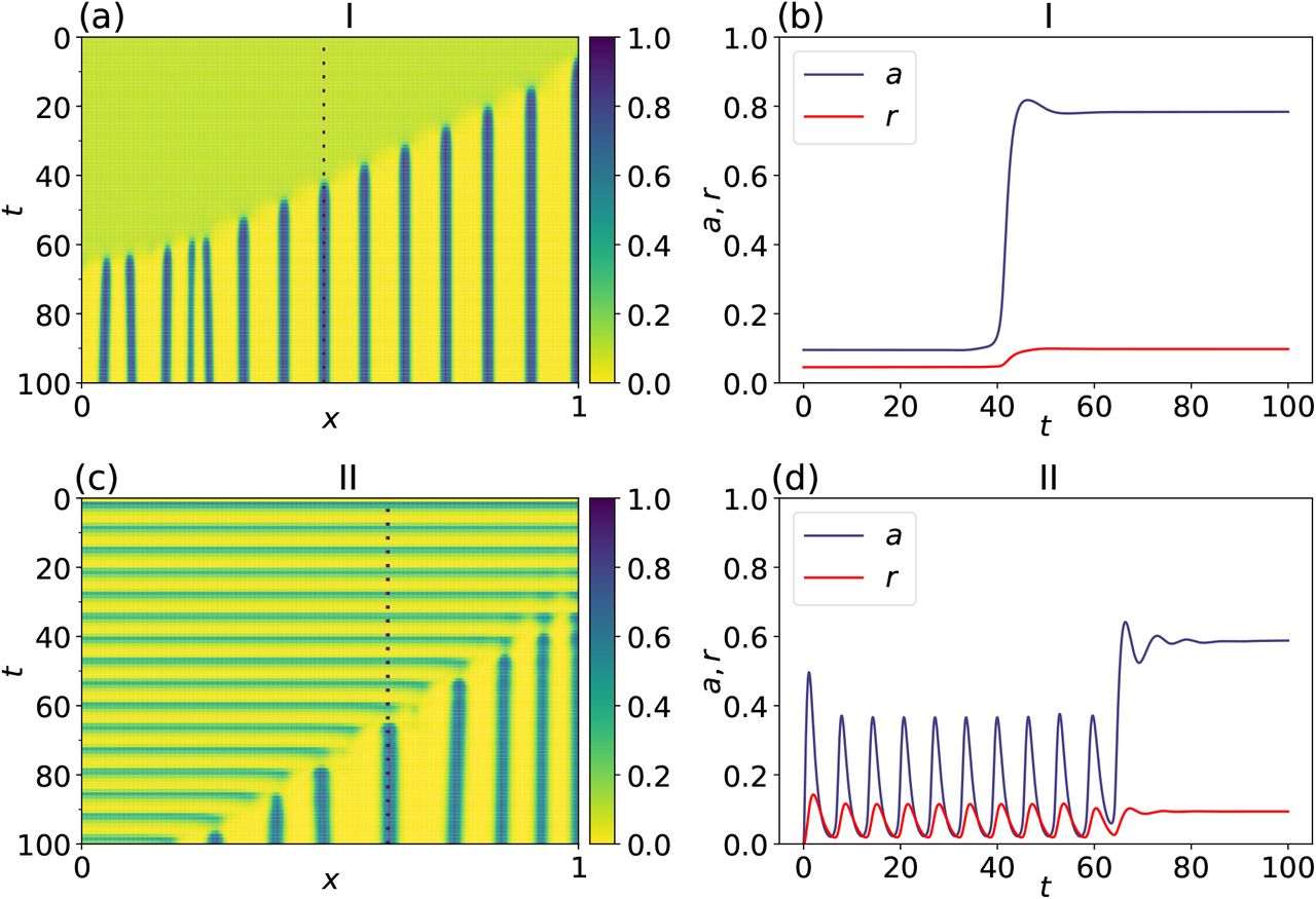
Time-step simulations of (A.3) with homogeneous Neumann boundary conditions and parameter set values as in region I and II plotted in Fig. A.2. An azimuthal view of the spatio-temporal solution shows the pattern formation dynamics for a Turing type (panel a) and a Turing-Hopf type (panel c). Temporal evolution for each case in the left-hand side column of the activator and repressor at x = 0.6125 and x = 0.4875 (dashed lines in panels a and c) are shown in panels (b) and (d), respectively. Initial conditions were taken as a perturbation of the steady state accordingly to regions I and II, respectively, of the parameter space in Fig. A.2.
The four kinds of patterns depicted in Fig. A.2 are classified according to the roots of (A.7). A sample of each root-solution type is plotted in Fig A.3, where solid lines are the real part of the eigenvalues and the dashed lines correspond to the imaginary part. The Turing pattern region is labelled by I; as can be seen there, the dispersion relation has a finite positive maximum which gives place to an interval of unstable wave modes. For region II, a Turing-Hopf pattern dispersion relation is depicted, where the imaginary part is non zero for positive portions of the real part, and when the imaginary part colapses to zero, the real part is as in the Turing region. That is, this stability feature gathers two main dynamical ingredients: oscillatory and non oscillatory unstable modes in two finite disconected subintervals. In region III, a Hopf pattern is characterized by having a dispersion relation in which the real part is only non negative for wave modes where the imaginary part is non zero. Finally, region IV corresponds to no pattern, which is characterized by having a negative real part of the dispersion relation for all wave modes, and hence the homogeneous steady state suffers no symmetry breaking. In other words, the combination of real and imaginary parts of λ(κ2) in (A.4), and provided by (A.6), determines each pattern type as well as transitions between regions. For a detailed discussion about the former approach, see (Liu et al., 2007).

Simulations with parameter β as function of x and t as indicated in the text. For (a), the initial conditions are perturbations of the steady state, while in (b) the initial conditions are the final state of (a).
Regions I and II are particularly relevant as a stationary pattern is formed, although a key mark lies on transitory dynamical behavior for each scenario. To illustrate this distinguished mark, we perform time-step runs for a setting in both regions, by having a perturbed steady state as an initial condition; see top panels in Fig. A.4. As can be seen in panel (a), the system is initially in a homogeneous steady state with a slight perturbation. As time goes by, a heterogeneous pattern arises. This is a consequence of the unstable wave modes as is shown in Fig. A.3, panel (b), which corresponds to the Turing pattern, region I, in Fig. A.2. In addition, in panel (b), a time evolution is observed for the activator and repressor states at x = 0.6125. On the other hand, in an analogous fashion, the transitory dynamics spontaneously oscillate as a consequence of the non zero imaginary part of λ(κ2). Such oscillatory dynamics goes on until unstable wave modes allow a stationary pattern to arise. Notice that this mark is clearly observed in panel (d); see bottom panels in Fig. A.4. In other words, even though both dynamical configurations give place to stationary patterns, the crucial oscillating feature previous to finally get a fixed pattern is added by having a Turing-Hopf mechanism in play.
In Fig A.5, we show additional results, where a spatio-temporal dependent parameter β is taken into consideration. There, we take β as in (8) where v = 0.02 and v = −0.02 for the run in panels (a) and (b), respectively. The initial conditions for panel (b) corresponds to the final profile of panel (a). Notice that once the pattern is completely formed, even though β varies in a inverse direction, the pattern is not destroyed. This is typical trait of a hysteretical process. In other words, this result indicates that the proposed mechanism is robust since, once the wave front depicted by β in (8) prompts the formation of somites, this process cannot be undo.
References


