

Abstract
Arthropod segmentation and vertebrate somitogenesis are leading fields in the experimental and theoretical interrogation of developmental patterning. However, despite the sophistication of current research, basic conceptual issues remain unresolved. These include (1) the mechanistic origins of spatial organisation within the segment addition zone (SAZ); (2) the mechanistic origins of segment polarisation; (3) the mechanistic origins of axial variation; and (4) the evolutionary origins of simultaneous patterning. Here, I explore these problems using coarse-grained models of cross-regulating dynamical processes. In the morphogenetic framework of a row of cells undergoing axial elongation, I simulate interactions between an “oscillator”, a “switch”, and up to three “timers”, successfully reproducing essential patterning behaviours of segmenting systems. I also compare the output of these largely cell-autonomous models to variants that incorporate positional information. I find that scaling relationships, wave patterns, and patterning dynamics all depend on whether the SAZ is regulated by temporal or spatial information. I also identify three mechanisms for polarising oscillator output, all of which functionally implicate the oscillator frequency profile. Finally, I demonstrate significant dynamical and regulatory continuity between sequential and simultaneous modes of segmentation. I discuss these results in the context of the experimental literature.
1 Introduction
Arthropod segmentation [1] and vertebrate somitogenesis [2, 3] are paradigmatic examples of developmental pattern formation. They involve the coordination of diverse cellular processes – signalling, gene expression, morphogenesis – yet can be conveniently abstracted to a single dimension, making them conducive to mathematical modelling and theoretical analysis.
The spatial patterns produced by segmentation processes have at least three components (Fig 1A). First, periodicity – the reiterated nature of individual metameres. Second, the intrinsic polarity of these units, evident in the expression of segment-polarity genes. Finally, regionalisation – variation in the length and identity of metameres according to their position along the anteroposterior (AP) axis. Segmentation patterns are highly robust within species [4–6] but evolutionarily flexible between species [7–10], with differences in the number, sizes, and specialisation of segments contributing to the considerable morphological diversity of segmented clades.

A: Three components of AP patterning. B: Three mechanisms for spatial pattern formation. Left: organisation emerges in an initially homogenous tissue by local reaction and diffusion. Middle: an embryonic field (white) interprets positional information (red line) to acquire positional values, and subsequently differentiates (coloured domains). Right: a wavefront (white line) moves across a tissue as it matures from an early state (red) to a late state (blue), and freezes the temporal pattern in space. C: Diagram of a model simulation, see text for details. Red lines = posterior signalling centre, light red domains = range of signal. D: The three “dynamical modules” used in the models. A timer has a duration T. An oscillator has a hidden phase (grey dotted line), an output level (blue line) and a period, P. A switch has n mutually exclusive states (here n = 3) that are activated by particular input conditions. Module behaviours are assumed to derive from underlying cellular regulatory networks, including (for example) AC-DC motifs [62] (left), autorepression (middle), or mutual repression (right).
Segment patterning emerges, in most species, from fundamentally temporal developmental mechanisms. In both vertebrates and arthropods, temporal periodicity is generated by a “segmentation clock” (molecular oscillator), then translated into spatial periodicity by a “wavefront” of cell maturation that sweeps the elongating AP axis from anterior to posterior at a tightly controlled rate [11–15]. These tissue-scale dynamics are generated, at the molecular level, by the characteristic rates, time delays, and flow properties of intercellular and intracellular regulatory networks [16–21], in combination with morphogenetic processes [22–24].
Genetic, environmental, and pharmacological perturbations can alter the segment pattern [13, 25–35], providing insight into its mechanistic basis. However, despite the experimental sophistication of vertebrate research in particular, these approaches are often constrained by functional redundancy and pleiotropic effects. Modelling studies provide a complementary way to interrogate segmentation processes, and have produced important conceptual advances [11, 16, 36, 37]. Yet a range of modelling approaches with contrasting regulatory bases have been able to give more or less convincing approximations of empirical observations, and it can be unclear how to best choose between them [37–48].
In this context, it is a worthwhile exercise to step away from the particularities of specific genes, signals, and experimental species, and consider the generic ramifications of basic assumptions. Here, I identify four aspects of the segmentation process where the nature of patterning is open to question or unclear. I then explore each of these issues using coarse-grained, illustrative models, in which potentially complex processes are represented by interactions between phenomenological “dynamical modules”. Finally, I discuss the implications of these results in the context of the experimental literature.
2 Patterning problems in segmentation
2.1 Sources of spatial information
Developmental patterning requires that cells’ state trajectories (changes in internal state over time) are influenced by their location – either their global position within the tissue or embryo, or their local position relative to certain other cells. In other words, some cell state variable must respond to a source of spatial information, and different values for this variable must cause otherwise identical cells to diverge in fate. Three general mechanisms that accomplish this have been identified:
Self-organisation (i.e. reaction-diffusion) mechanisms [49–51] (Fig 1B, left), in which small heterogeneities between cells, perhaps originating ultimately from stochastic fluctuations, are amplified by coupled positive and negative feedback loops into regular spatial patterns with a characteristic length scale. The key here is that the feedback loops and diffusive processes effect a local exchange of state information between cells, so that state trajectories become dependent on relative position.
Positional information (PI) mechanisms [52–54] (Fig 1B, middle), in which a polarised scalar variable (e.g., the concentration of a graded morphogen) provides a coordinate system for a bounded embryonic field. Cells “interpret” the positional information to acquire a “positional value”; the value serves as a proxy for a cell’s position within the field, and influences its subsequent state trajectory. PI processes are constrained by the accuracy and precision with which the PI signal is established and interpreted.
Time-space-translation (TST) mechanisms [11, 55–59] (Fig 1B, right), in which a tissue-scale velocity converts a temporal pattern into an isomorphic pattern arrayed across space. The velocity (i.e., a wave of gene expression across a field of cells, or a flow of cells relative to the source of an extracellular signal) causes cells at each position to experience a particular input at a different time relative to ongoing changes to cell state, with correspondingly different effects on cell fate.
These modes of patterning are conceptually distinct, but are unlikely to be cleanly dissociable in real systems. Cell states change constantly as the result of intrinsic processes (e.g., the synthesis and turnover of gene products) and extrinsic influences (e.g., the transduction of extracellular chemical and mechanical signals), and, in an embryonic context, thousands of cells respond to each other’s signals and move relative to one another simultaneously. The massively parallel feedback loops between cell state, signalling and morphogenesis, occurring over a wide range of timescales and lengthscales [60], mean that non-trivial developmental phenomena are unlikely to be governed by a single patterning mechanism, but will instead emerge from a recursive blend of self-organisation, PI, and TST. The challenge of developmental biology is to unpick these processes and render the whole system comprehensible. Indeed, perhaps it is in the interactions between patterning mechanisms that explanations for developmental robustness and evolutionary flexibility are to be found [61].
2.2 SAZ organisation and the “determination front”
With some significant exceptions (see below), segmentation occurs in the context of posterior elongation, with segments/somites emerging sequentially from the anterior of a segment addition zone (SAZ, arthropods) or the presomitic mesoderm (PSM, vertebrates). [Unless otherwise indicated, “SAZ” is hereafter used as a generic term that encompasses both SAZ and PSM.]
In both arthropods and vertebrates, the posterior tip of the SAZ continuously moves away from more anterior structures, either by a mix of convergence extension movements and cell proliferation (arthropods) [63–67], or by cell influx, cell proliferation and a greater motility of posterior vs anterior cells (vertebrates) [24, 68–73]. These processes, and therefore the maintenance of axis elongation, depend directly or indirectly on a posterior signalling centre (PSC) involving Wnt signalling, itself maintained by positive feedback loops [30, 74–84]. The posterior signalling environment maintains SAZ cells in an immature, unpatterned state, preventing their differentiation into segmental fates [28, 30, 85–89].
The more anterior the location of a cell within the SAZ, the more remote it is from the PSC, both in terms of physical distance, and in terms of time. (Note that the SAZ is a dynamic structure through which there is a continuous flux of cells.) At a certain point within the SAZ, cells undergo a significant state transition, and begin expressing different sets of transcription factors (e.g., Odd-paired rather than Dichaete/Sox21b and Caudal in arthropods [15, 84, 89–94]; Paraxis/TCF15 vs Mesogenin, and a combinatorial code of T-box factors in vertebrates [29, 95–100]). This transition coincides with the specification of segmental fate, at least partially because the transcription factors on either side of it differentially regulate segmentation gene enhancers [98, 101–106]. This transition or “determination front” [13] can therefore be identified with the wavefront of the clock and wavefront model.
The positioning of the determination front – and the origins of spatial organisation within the SAZ more generally – is fundamental to the control of segmentation. It is clear that SAZ geometry is affected by the levels of Wnt and other signals within the embryo [3, 107]. What is less clear, however, is the respective role played by spatial and temporal information in producing these outcomes. The more anterior a cell is, the further it is from the PSC and the closer it is to patterned tissue that may produce antagonistic signals such as retinoic acid [108]. However, it will also have spent a longer time degrading posterior signals [28, 30, 109] and potentially undergoing other autonomous changes in cell state. Because temporal and spatial coordinate systems are overlaid on one another in this way, they are extremely difficult to disentangle.
There are two distinct regulatory questions here. The first, and simplest, asks to what extent the signalling environment along the SAZ is shaped by position dependent, diffusive effects, as opposed to advection (bulk transport) and temporal decay [44]. While both play some role, the latter effects appear to dominate in embryos. For example, Wnt perturbations take hours to affect somitogenesis in zebrafish, with effects on SAZ gene expression travelling from posterior to anterior at the rate of cell flow [87], and dissected PSM tissue generally maintains an endogenous maturation and patterning schedule [110–113]. Despite this, most segmentation models assume that SAZ patterning is governed by a characteristic lengthscale, rather than by a characteristic timescale.
The second question, less frequently raised, concerns the relationship between the signalling levels a cell experiences, and the dynamics of its internal state. Most segmentation models implicitly assume a PI framework, in which a cell moves within a PI field, continuously monitoring a graded signal, until a particular positional value induces a change in cell state [37, 39, 45, 47, 114, 115]. (Other models propose that cells actually respond to a different property of the field [42, 46], but the basic principle of decoding a PI signal remains the same.) An alternative hypothesis is that cells will autonomously travel along a maturation trajectory from a “posterior” state to an “anterior” state over a period of time, with the signalling environment governing the rate of cell state change, but not determining cell state per se.
The two hypotheses predict quite different behaviour: The former suggests that intermediate states are stable in the appropriate signalling environment and that cell maturation is associated with the decoding of a specific external trigger; The latter suggests that intermediate states are inherently unstable and that signalling levels and cell state can be partially decoupled. Significantly, recent results from stem cells and ex vivo cultures support the latter hypothesis by pointing to an important role for cell-intrinsic dynamics: stems cells in constant culture conditions will transition from a posterior PSM-like state to an anterior PSM-like state over a characteristic period of time [100, 116, 117], while more anterior PSM cells will oscillate slower than posterior PSM cells in otherwise identical culture conditions [118].
Thus, the emphasis in the modelling literature on SAZ lengthscale and morphogen decoding is at odds with empirical findings. However, because much of axial elongation can be approximated by a pseudo-steady state scenario [37] in which the dimensions of the SAZ remain constant and spatial and temporal coordinate systems coincide (and are therefore proxies for one another), timescale-based and lengthscale-based models will often yield similar predictions. A central aim of this study is to explicity contrast these two patterning frameworks and determine their characteristic implications.
2.3 Prepatterns and polarity
Segments and somites both have an inherent polarity, but their polarity manifests in different ways. In arthropods, the segmentation process generates a segment-polarity repeat with three distinct expression states (i.e., anterior, posterior, and a buffer state in between), with polarised signalling centres forming wherever the anterior and posterior states abut [119–123]. These signalling centres demarcate the boundaries of the future (para)segments, and later pattern the intervening tissue fields by a PI mechanism [124–127].
In vertebrates, the segment-polarity pattern is just a simple alternation of anterior and posterior fates [128, 129], and it is not necessary for boundary formation per se [130–132]. Instead, somitic fissure formation depends on the relative timings of cells’ mesenchymal to epithelial transition (MET) and differences in their functional levels of specific extra-cellular matrix (ECM) components such as Cadherin 2 (CDH2) [133]. These properties are modulated by the segmentation clock [134, 135], which explains the regularity, scaling properties, and species-specificity of somite size, as well as the tight coordination between somite boundary formation and the segment polarity pattern. However, note that there is spatial information in the ECM pattern that is absent from the segment-polarity pattern [136] — this explains why the somitic fissures that gate cohorts of cells into coherent morphological structures form only at P-A interfaces, and not also at the A-P interfaces in between, as would be predicted by a prepattern mechanism.
Thus, arthropod segments are polarised because their morphogenesis is specified by a polarised prepattern, while vertebrate somites are polarised because morphogenesis intersects with a non-polarised prepattern in a polarised way. However, in both cases the origin of this polarity still needs to be explained. In all vertebrates and at least some arthropods, the segmentation clock is thought to be based around coupled oscillations of her /hes gene expression and Notch signalling [26, 27, 36, 88, 137–147]. Both theoretical models and empirical data suggest that such networks generate sinusoidal oscillations, which are not inherently polarised [16, 42, 88, 116, 142, 148, 149]. The problem thus arises of how a non-polarised pattern in time is able to specify a polarised pattern in space. I will present two strategies for how this could be achieved, one inspired by data from arthropods, and the other by data from vertebrates.
2.4 Axial variation and scaling
In real embryos, elongation, SAZ maintenance and segmentation eventually terminate, usually all at roughly the same time, after the production of a species-specific and relatively invariant number of segments [97, 150]. These segments often have different sizes and molecular identities according to their axial position; for example, tail segments are usually smaller than trunk segments and express more 5’ Hox genes. Understanding how segmentation “profiles” are generated requires determining (1) which parameters of the segmentation process are modulated to produce axial variation and terminate segment addition, and (2) how the dynamics of these parameters are controlled.
Segment identity and segmentation duration
In both vertebrates and arthropods, segment identities are specified by sequentially expressed Hox genes [151–155]; in at least some arthropods, Hox gene expression is regulated by another set of sequentially expressed transcription factors, encoded by the gap genes [156, 157]. Hox and gap gene expression is established in parallel with, but independent of, segment boundary patterning. Indeed, segment number and segment identity can be decoupled by various perturbations [19, 32, 158–160].
Hox and gap gene expression is activated by posterior factors such as Cdx and Wnt [89, 161–164], and the individual genes also cross-regulate each other’s expression. Thus Hox and gap gene expression depends partly on the state of the SAZ and partly on intrinsic dynamics [56, 165–167]. As well as generating regionalisation information, the sequential expression of these genes affects segment patterning, because late-expressed Hox and gap genes antagonise SAZ maintenance and axial elongation [77, 168–170].
Reaction-diffusion processes [44, 45, 150] could additionally play a role in controlling the duration of segmentation, as could the proliferation rate and initial size of unpatterned tissues [71, 171]. Thus, segmentation termination is likely controlled by some kind of effective timer, but it is not clear whether this timer resides in the dynamical properties of a particular gene network, or is broadly distributed in the system at large.
Segment size control
In a clock and wavefront framework, segment length is determined jointly by clock period and wavefront velocity [11, 37]. Both parameters change over the course of embryogenesis [86, 97, 150, 172], but the change in oscillation period is opposite of that expected from changes in segment size, increasing at late stages while segment sizes decrease. Thus, variation in the clock is more important for explaining segment size variation between species [21, 97, 173, 174] than the size variation in an individual embryo over time. In addition, oscillator period is unaffected by embryo size variation, although embryo size is tightly correlated with segment length [45]. Therefore, variation in segment size over time and between individuals must be largely a consequence of variation in wavefront velocity.
The wavefront velocity should be similar to the elongation rate, and would also be affected by any temporal changes to SAZ size, which would require it to move faster or slower than elongation to make the adjustment [149]. The regulation of elongation rate and SAZ size is therefore of fundamental importance to understanding the segment profile. Are changes to these properties linked to Hox gene expression changes or independent of them? Are elongation rate and SAZ size controlled separately or are they mechanistically linked? What accounts for observed scaling relationships between segment size, SAZ size, and oscillator wave patterns [5, 42, 45, 97, 149, 172]? Within species, these relationships are broadly (though not entirely [175, 176]) conserved between individuals, despite variation in embryo size and temperature-dependent developmental rate. At the same time, they vary moderately within individuals over the course of segmentation, and can vary dramatically across species.
Determining the upstream temporal regulation and proximate mechanistic causes of axial variation is central to questions of developmental robustness and evolutionary flexibility. At the same time, by providing a more exacting set of observations for segmentation models to explain, the investigation of these issues should also generate considerable insight into the control of segmentation at “steady state”. I will demonstrate this point by showing that the downstream effects of temporal variation in elongation rate or SAZ size depend on whether the SAZ is patterned by spatial or temporal information.
2.5 Simultaneous segmentation and its evolution
Finally, in several groups of holometabolous insects (including the best studied segmentation model, Drosophila) the ancestral segmentation process has been modified by evolution to such an extent that it is almost unrecognisable [177]. The segmentation clock has been replaced by stripe-specific patterning by gap genes [178–183], while segments mature near-simultaneously at an early stage of embryogenesis, rather than sequentially over an extended period of time. Contrasting with the temporal nature of clock and wavefront patterning, the Drosophila blastoderm has become one of the flagship models of positional information [184–186].
Yet, in recent years it has been found that many of the dynamical aspects of Drosophila segmentation gene expression are strikingly reminiscent of sequential segmentation. For example, domains of gap gene and pair-rule gene expression move from posterior to anterior across nuclei over time [123, 187–191], while the timing of pattern maturation is regulated by factors associated with the SAZ in sequentially-segmenting arthropods [15, 106, 192]. At the same time, there have been several experimental results that belie a strict PI framework, such as those characterising the activation thresholds of Bicoid target genes [193, 194], or the information content of maternal gradients [184, 185, 195].
Clarifying the regulatory homologies between simultaneous and sequential segmentation and determining the functional significance of Drosophila segmentation gene dynamics will shed light on both simultaneous and sequential segmentation processes, as well as the evolutionary trajectories between them. I propose a general framework for this below.
3 Modelling framework
The four issues described above – (1) the origins of spatiotemporal order within the SAZ, (2) the origins of segment polarisation, (3) the proximate and ultimate regulatory causes of axial variation, and (4) the existence of extreme transmogrifications of the segmentation process – are as much questions about the origins and transformations of spatial information as they are questions about particular biological mechanisms. To focus attention on spatial information, I have chosen to use a modelling framework that simulates the dynamics and interactions of regulatory processes within cells but remains agnostic as to their molecular implementation. To easily follow the logic of patterning, the models are simple, uni-dimensional, and deterministic.
Unlike models that explicitly specify the properties of the patterning field, here the emphasis is on internal cell state and on autonomously-driven cellular dynamics. An “embryo” is modelled as a 1D array of largely autonomous “cells”; the state of each cell is represented by a vector of state variables, each of which represents a particular “dynamical module” (Fig 1C). For simulations, I use discrete time and synchronous update: the state of a cell at tn+1 is calculated from its state at tn according to pre-specified regulatory rules, which are identical for all cells.
Each dynamical module represents a set of cellular components, such as a cross-regulatory gene network, that executes a coherent dynamical behaviour. The modules may be of three general types. A “timer”, τ, (Fig 1D, left) decreases from an initial state 1 to a final state 0 at rate 1/T (where T is the timer duration in timesteps). [N.B., this is just an abstract representation of a canalised cell state trajectory and should not be confused with linear decay of a particular gene.] An “oscillator”, o, (Fig 1D, middle) generates a sinusoidal output: it has a hidden phase value ϕ [0, 1] which advances at rate 1/P (where P is the period in timesteps), and is converted to a functional output level by the function o = (sin(2π(ϕ − 1/4))+1)/2. Finally, a “switch”, s, (Fig 1D, right) remains at an initial state 0 until one of n mutually exclusive states is activated by a rule. Each module may additionally be regulated by the current state of one or more different modules, allowing for flexible context-specific behaviour.
Each embryo has an initial length L0 (usually 1 cell) and a polarity defined by a posterior signalling centre (PSC) that is extrinsic to the row of cells. The PSC emits a Boolean posterior signal that has a spatial range of r cell diameters. The signal can affect cell state by entering as a variable in the regulation of a dynamical module. It also induces embryonic elongation. Elongation is effected within the model by duplicating the posterior-most cell (including all its state variables) at regular time intervals determined by an elongation rate v (e.g., if v = 0.2 the embryo adds a cell every 5 timesteps). Each increase in embryonic length posteriorly displaces the PSC by one cell diameter, freeing the (L − r)th cell from its influence. Note that this elongation mechanism is just a modelling convenience, representing any of cell proliferation, cell rearrangement, or cell recruitment.
For many of the simulations, no other morphogenetic or cell communication processes are included, and initial conditions are identical between cells. As a consequence, the elongation-driven dynamics of the posterior signal (i.e., a velocity) is the sole source of spatial information in the system; all patterning must occur via TST (time-space translation). In other simulations, cells are allowed to calculate their spatial distance from the posterior signal or to have different initial conditions, introducing PI effects. Self-organisation effects are excluded from the models so as to more clearly contrast PI and TST, but they are undoubtedly important in real segmenting tissues, particularly for counteracting stochasticity.
The series of models that I investigate is summarised in Fig 2. Mathematical details are provided in a supplementary document.

Dynamical modules are shown as coloured boxes, other model features are shown as white boxes. Regulatory connections are indicated with arrows.
Table of model symbols.
4 A clock and timer model
The first model (Fig 2A) presents a simple clock and wavefront scenario, which will be iterated on in later sections. Here, the main concern is establishing the basic logic of the model and understanding the effect of each parameter on model behaviour. I contrast two variants of the model, one in which the SAZ is patterned by temporal information, and another in which the SAZ is patterned by spatial (positional) information. Their patterning output is overall similar, but they are differently affected by the elongation rate.
The temporal variant of the model involves a timer, an oscillator, and a switch. The timer represents cellular maturation from an undifferentiated (posterior SAZ) state to a differentiated (anterior SAZ) state. The oscillator represents a segmentation clock. Finally, the switch represents a binary choice between anterior and posterior segment polarity fates.
The timer is maintained in its initial state (1) by the posterior signal. Once this signal is removed, the timer decreases at rate 1/T until it reaches its ground state (0). When the timer reaches 0, it triggers a hand-over from the oscillator (expressed only when τ > 0) to the switch (expressed only when τ = 0), with segment-polarity fate (switch value) determined by the final oscillator level as it turns off (1 if o > 0.5; 2 otherwise). In addition, the frequency of the oscillator is modulated by the timer: a lower timer state causes slower oscillations (Fig 3E)*. The regulatory interactions between the modules reflect, in simplified form, those between PSM TFs (the timer), the hes/Notch segmentation clock (the oscillator) and mesp segment polarity genes (the switch) in vertebrate somitogenesis, as inferred from genetic perturbations and functional analysis of enhancers [103–105, 198, 199]. (In arthropods, the interactions between SAZ TFs, oscillating genes, and segment-polarity genes are likely to be similar but slightly more complicated, as described in the section below.)

A: Example simulation output, for the parameter values and timepoints shown. Only one switch state is plotted. B: Faster oscillations (smaller P) produce shorter segments. C: A slower timer (larger T) produces a longer SAZ. D: Faster elongation (larger v) produces longer segments and a longer SAZ. E: Oscillator frequency is scaled by (1 − e−2τ)/(1 − e−2). F: “Temporal” model variant: timer state is a function of time. G: “Spatial” model variant: timer state is replaced by a PI value, which is a function of distance. H: SAZ length scales with elongation rate in the temporal model variant but not the spatial variant. I: SAZ length scales with both timer duration and PI lengthscale. J: Segment length is unaffected by timer duration or PI lengthscale. K: SAZ phase difference is independent of elongation rate in the temporal variant, but not in the spatial variant. L: SAZ phase difference scales with both timer duration and PI lengthscale. M: SAZ phase difference scales with oscillator frequency in both model variants. SAZ length = number of cells where τ > 0, excluding signal-positive cells; Δ phase = oscillator phase difference between anterior and posterior of SAZ; solid lines = temporal model variant; dashed lines = spatial model variant.
When simulated, the model generates typical “clock and wavefront” behaviour (Fig 3A, Movie 1). Because the state of the timer in a given cell is a function of the time since that cell last saw the posterior signal (Fig 3F), elongation generates a dynamic gradient of timer state along the AP axis (i.e., a temporal co-ordinate system), which moves posteriorly in concert with the posterior signal. Fast, synchronous oscillations are maintained in the posterior of the embryo (where τ = 1); these narrow into anteriorly progressing kinematic waves where 0 < τ < 1. Finally, segment polarity expression is activated stably in a smooth A-P progression, as the “determination front” (τ = 0) moves posteriorly at a steady rate. As expected [37], segmentation rate matches the oscillation period in the posterior of the embryo, and segment length depends jointly on the oscillator period and the elongation rate (Lseg = P ∗ v) (Fig 3B,D).
The inclusion of the timer in the model means that cells are destined to autonomously follow a particular temporal trajectory once they are relieved from the posterior signal. Thus, the spatial organisation of the SAZ is a reliable by-product of elongation, but plays no explicit role in cell regulation. Alternatively, segmentation dynamics could be under the control of a PI system: the SAZ would be associated with a typical lengthscale λ, and a cell’s behaviour would depend explicitly on its position within the SAZ field. In the “spatial” variant of the model, the timer is replaced by a state variable that is a function of a cell’s distance from the posterior signal (Fig 3G), and the same downstream effects are retained.
Although these model variants are conceptually distinct, they generally predict very similar behaviour. In both cases, the progression of the wavefront is powered by elongation – either because it causes increasingly posterior cells to set their timers in motion at increasingly advanced timepoints (the temporal variant), or because it causes the whole SAZ field to retract along with the posterior signal (the spatial variant). Whether cell maturation is governed by a characteristic timescale (T, temporal variant) or by a characteristic lengthscale (λ, spatial variant), segment length is determined only by P and v (Fig 3J). In addition, SAZ length scales linearly with either T or λ (Fig3I; compare 3A with 3C), as does the oscillator phase difference across the SAZ, which determines the number of SAZ stripes (Fig 3L; compare 3A with 3C). The phase difference also scales with oscillator frequency in both models (Fig 3M; compare 3A with 3B).
However, the two variants respond differently to elongation rate (Movie 2). With a timer, SAZ length is proportional to elongation rate (LSAZ = T ∗ v; compare 3A,C,D), but with a PI system SAZ length depends (by definition) only on λ (Fig 3H). Furthermore, with a timer the SAZ phase difference is essentially independent of elongation rate (compare 3A,D), but with a PI system slower elongation is associated with an increasing number of stripes (Fig 3K). A timer-based system therefore naturally predicts scaling of SAZ length with elongation rate and scaling of wave dynamics with SAZ length, while a PI-based system does not.
5 A clock and two timers
The next model examines how a more complex segment-polarity pattern could be generated. Arthropods generate at least three states (Fig 4B) for every segmentation clock cycle, instead of just two states as in vertebrates (Fig 4A). Some groups of arthropods (insects, centipedes), pattern two segments for every oscillator cycle [14, 200], and must generate a pair of triplet repeats (i.e., six states, Fig 4C).†

A-C: Symmetric (A) and polarised (B,C) inputs and potential output patterns. Green=anterior fate, grey=posterior fate, white=middle fate, orange=alternative anterior fate. D: Peaks from a symmetric input reset a timer, producing a polarised output. Network diagram shows a possible underlying network topology: an oscillatory gene represses the later-expressed nodes of an AC-DC circuit “timer”, forcing it from stable end-state to unstable start-state. E-H: Example simulation output, for parameter values shown (note that T2 duration is identical for all simulations). E: 3-state timer-switch mapping, as in B. F-H: pair-rule mapping, as in C. E,F: P ∼= T2. G: P > T2; final state expands. H: P ∼= T2/2; only the first half of the pattern is ever generated. I: Timer 2 and oscillator dynamics are identically affected by timer 1. J: Only the oscillator is affected by timer 1. K,L: Simulation output kymographs showing timer 2 state (diagonal pulses) and switch output (vertical stripes) when T2 is moderately larger than P, and the timer 2-switch mapping consists of three equally-sized states. White=1, black=0. K: profiles in I are used; the posterior state is narrower than the others. L: profiles in J are used; the posterior state is wider than the others. M: Difference between the timer states in K and those in L. Darker shade indicates greater difference. Note that the states diverge towards the anterior of the SAZ. N: Ratio of output pattern lengthscale to segment length for simulations with different timer 1 durations, using the profiles in I (same) or the profiles in J (diff.). Black dots show individual simulations, grey lines show fitted polynomials. Deviations are due to the discrete nature of the output.
If cells are able to calculate “where” they are within an oscillation cycle (i.e., oscillation phase), it is theoretically possible to generate a segment-polarity pattern of arbitrary complexity, simply by changing the mapping between the input phase values and the output switch states. For example, two input thresholds are needed for a three-state pattern, and five thresholds are needed for a pair-rule pattern. The trivial way to implement this is to allow cells direct access to the oscillator phase variable that is “hidden” in the clock and timer model just described. Unambiguous phase determination would be possible, for example, if the segmentation clock was a multi-gene “ring oscillator” [201], because each portion of the phase would correspond to a unique combination of transcription factor concentrations. Under this scenario, the segment-polarity pattern would always scale with segment length.
However, suppose the core oscillator is based on direct her /hes gene autorepression, as is the case in vertebrates [202], and potentially arthropods as well [1]. Now there is no one-to-one mapping between oscillator output (i.e., concentration level) and oscillator phase, because oscillator output both increases and decreases over the course of a cycle. (This is the motivation for hiding the phase variable from the other modules — phase would be implicit in the combination of oscillator transcripts and proteins present in a cell, but not determinable from the protein level alone.) For cells to unambiguously determine their position within a oscillator repeat, they must compute phase information from the oscillator’s dynamics.
Suppose an additional timer module is inserted into the model, to mediate the interaction between the oscillator and the switch (Fig 2B). Let the original timer be “timer 1” (τ1), and the new timer “timer 2” (τ2). Timer 2 represents various pair-rule gene transcription factors (other than hairy, which I am assuming is associated with the oscillator) expressed in the arthropod SAZ (Fig 4D, top) [1, 92, 201, 203]. Like the oscillator, timer 2 can only be expressed where τ1 > 0, and so is similarly restricted to the SAZ. It also receives periodic input from the oscillator: when oscillator levels are at their peak (above a threshold θ = .995), timer 2 resets to its initial state (1), else it decreases at rate 1/T2 until it reaches its ground state (0). Timer 2 therefore measures the time since the oscillator was last at its peak; note that this effectively digitizes the analog oscillator signal to peak (on) vs non-peak (off) (Fig 4D, bottom.) If T 2 is of similar magnitude to P, the state of timer 2 makes a good proxy for oscillator phase, and can be used to specify a polarised pattern (Fig 4E,F, Movie 3).
However, because the oscillator and timer 2 each have their own characteristic timescale, segment length and segment pattern are no longer inherently coupled. If T2 < P, timer 2 has to wait some time at 0 before the oscillator hits its next peak, making the final state in the pattern repeat take up a larger proportion of the pattern. If the oscillator cycles with double-segment periodicity, this effect causes alternate segments to be different lengths (Fig 4G, Movie 3), as seen in some scolopendrid centipedes. Conversely, if T2 > P, timer 2 is always reset by the oscillator before it reaches 0, potentially meaning that posterior segment-polarity states are never produced. In an extreme case this could even change the periodicity of patterning from double-segmental to single-segmental (compare Fig 4F,H, Movie 3).
Above, it was found that the pattern generated by the clock and timer model was independent of the timescale of timer 1. This only holds for the clock and two timers model if the oscillator and timer 2 have the same frequency profile (Fig 4I,N). If the frequency profiles are different, the phase relationship between the oscillator and timer 2 will change across the length of the SAZ (Fig 4K-M). Longer values of T1 will result in a greater divergence between the two modules, and therefore the value of T1 will affect the segment pattern (Fig 4N).
6 A clock and timer with feedback
Decoding the phase of symmetrical oscillations is thus one mechanism to generate a polarised spatial pattern. An alternative mechanism is to use the TST process to modify the oscillations themselves. Periodicity would be generated by symmetrical temporal oscillations, as usual, but the spatial pattern recorded by the embryo would not be a faithful copy of this input.
The motivation here is to create a sawtooth spatial output, as seen for CDH2 in nascent somites. CDH2 levels affect cell adhesion, and boundary formation is favoured where low and high levels of CDH2 directly abut [204]. The segmentation clock establishes a smooth gradient of CDH2 across each nascent somite [134], with sharp high-to-low transitions prefiguring the somitic fissures [133, 136]. Strikingly, an ectopic fissure forms in the middle of each somite in mouse CDH2 mutants [205] (i.e., boundaries form at P-A and A-P transitions) suggesting this sawtooth pattern is instructive for polarised morphogenesis.
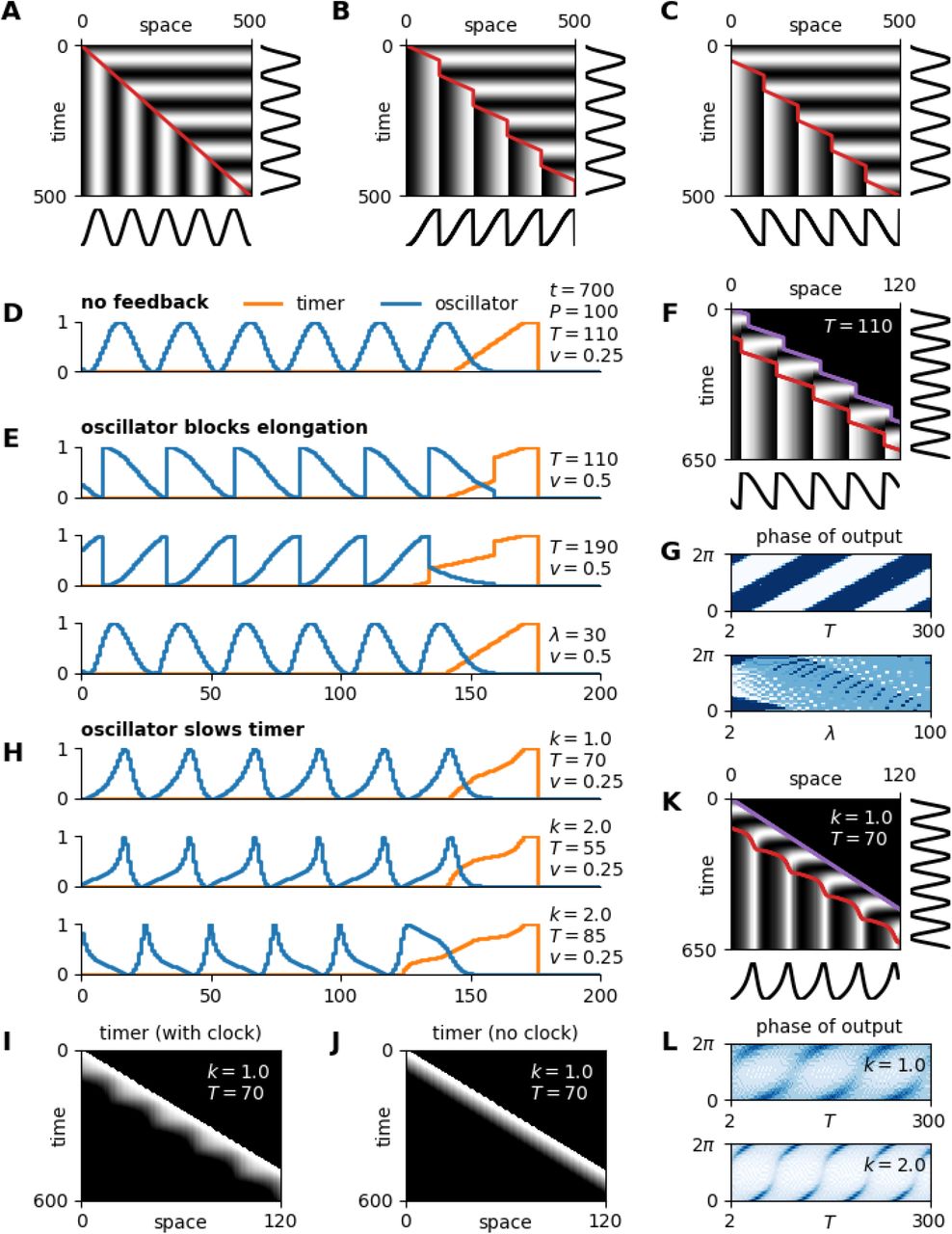
A symmetrical temporal pattern can only be transformed into a polarised spatial if the translation velocity varies over time. To illustrate the concept, suppose a wavefront is transcribing synchronous sinusoidal oscillations by freezing them in space (Fig 5A-C). If the wavefront velocity is constant (Fig 5A), the spatial output pattern is just the temporal input pattern scaled by the velocity. In other words, because the wavefront moves at a uniform rate, each section of the temporal pattern is given equal weight in the spatial output. If the wavefront velocity is variable, however, the output pattern will qualitatively change. If the wavefront moves faster or slower than average during some part of the oscillation cycle, the corresponding part of the input pattern will be stretched or compressed, respectively, in the output. If the wavefront pauses during part of the cycle, the corresponding section of the pattern will be skipped.

A-C: kymographs for a simple clock and wavefront system, with either a constant (A) or a variable (B,C) wavefront (red line) velocity. Temporal input and spatial output shown at right and bottom, respectively. D,E,H: example simulation output, for the model types and parameter values shown. F, K: simulation kymographs corresponding to the top rows of E and H, respectively. Purple line = embryo posterior; red line = anterior extent of the SAZ. G: output phase distributions for different timer durations (top, temporal model variant) or SAZ lengthscales (bottom, spatial model variant). I: kymograph of timer state, for the simulation shown in K. J: Equivalent to I, but with oscillator state maintained at 0. L: output phase distributions for different timer durations, when the oscillator’s effect on the timer is weak (top) or strong (bottom).
To extract a sawtooth pattern from the temporal signal, the wavefront would need to “transcribe” only half of the input pattern, stretch it to fill a whole segment length, and discard the rest – i.e., move at 2x speed for the first half of each oscillation cycle and pause for the second half (Fig 5B), or vice versa for reversed polarity (Fig 5C). (Note that the repeat length of the pattern is the same in all cases, but the lengthscale of the waves is doubled in Fig 5B,C as compared with 5A.) This patterning outcome requires that the wavefront velocity is strictly coordinated with both the oscillator period and the oscillator phase, suggesting that it could only occur in an embryo if there was feedback from the oscillator on the wavefront.
Sigificantly, pulsatile movement of the wavefront has been documented in vertebrates, and shown to be regulated by the segmentation clock [206–210]. In addition, zebrafish her1 gene expression has been described as showing a sawtooth pattern and a double-segment lengthscale as it arrests, rather than the expected sinusoidal wave [197], suggesting that the non-uniform wavefront dynamics do indeed result in oscillation polarisation.
I now modify the clock and wavefront model to show how these effects could arise. Consider a stripped-down version of the model that lacks the switch module (Fig 2C) and simply “freezes” the oscillator phase when the timer reaches 0, giving a clear readout of the transcribed pattern. With this basic set-up (Fig 5D), the wavefront moves at a constant velocity, the spatial output is isomorphic to the temporal input, and (as found earlier), neither the timer duration nor the oscillator frequency profile have any practical effect on the spatial output.
To affect the dynamics of the wavefront, the oscillator has to modulate either the elongation rate or the timer. Suppose first that the oscillator affects elongation: when the oscillator state in the posterior SAZ is below a threshold level (0.5) elongation proceeds as normal, but above this threshold elongation is suppressed. Axis extension now becomes coordinated with the segmentation clock (Fig 5F, purple line), as does the movement of the wavefront (Fig 5F, red line), and only half of the temporal input pattern is transcribed (Fig 5E,F, Movie 4). The phase range of the transcribed pattern depends on the amount that the oscillator state changes while a cell is relieved from the posterior signal but still within the SAZ, which is determined by the duration of the timer (Fig 5E, top vs middle and Fig 5G, top) as well as the period and the frequency profile (not shown). Interestingly, in the spatial variant of this model, where the timer is replaced by a PI field (recall Fig 3G), embryo elongation and wavefront velocity still show periodic dynamics, but the output pattern is hardly different from the temporal input (Fig 5E, bottom), except when the PI field is short (Fig 5G, bottom).
Suppose now that elongation rate remains constant but the oscillator affects the rate at which the timer state decreases. For example, let the timer rate be proportional to e−ko, where o is oscillator level and k is a parameter which determines the degree to which the timer can be slowed. Wavefront velocity now becomes decoupled from elongation rate (Fig 5K, compare the red and purple lines), in an oscillator-dependent manner (Fig 5I,J). Again, the spatial output pattern is qualitatively different from the temporal input generated by the oscillator (Fig 5K). The specific range of phase values that are recorded depends on both T and k (Fig 5H,L, Movie 5), as well as the period and frequency profile (not shown). In summary, any oscillator feedback on the wavefront could qualitatively affect the segmental pattern.
7 A clock and three timers
I now turn back to the clock and two timers model, and modify it to allow for axial variation and finite body length. Suppose a third timer (“timer 3”), representing Hox and/or gap gene dynamics, is added downstream of timer 1 (Fig 2D). Within the SAZ, timer 3 decreases from its initial state (1) to its ground state (0) at rate 1/T3. Outside the SAZ, timer 3 remains stable. As a result of TST, the timer 3 value of a mature segment provides a proxy measure of its axial position and could be used to specify its identity.
To modulate segment size and/or trigger segmentation termination, timer 3 should also affect the wave-front velocity, as previously discussed. This implies that it should modulate the elongation rate, and potentially timer 1.
Suppose the elongation rate depends on the state of timer 3, with the mapping between τ3 and v defined by a particular “growth profile” (e.g. Fig 6A -C). The profile can be of arbitrary shape but should fall to 0 when τ3 = 0, thereby terminating axis extension and segment addition. As intuitively expected, the segment size distribution produced by the system mirrors the growth profile (Fig 6A-C, Movie 6), and the final length of the axis (and therefore the final segment number) depends on the magnitude of T3 (Fig 6C).

A-C: example simulation output, for parameter values, growth profiles (A’-C’) and timepoints shown. t=∞ indicates the segment pattern will no longer change. D,E: summary statistics over time for simulations using the elongate rates (grey lines) shown at top. Results from the temporal (black) and spatial (purple) model variants are both shown. Brown dots show the segment size as a fraction of the SAZ size (T1 + P)/2 timepoints earlier. F: summary statistics over time for a simulation using the timer 1 rates (orange line) shown at top. Colours as in D,E. G: summary statistics over time for a simulation combining the the elongation rates (grey line) and timer 1 rates (orange line) shown at top. Note that in D-G, initial simulation stages (where τ1 > 0 in all cells and the SAZ grows rapidly) are not shown.
However, the precise way that the system responds to a growth profile (i.e., elongation rate variation) depends on whether the SAZ is patterned by temporal or spatial information (i.e., whether timer 1 is governed by T1 or λ, respectively). For example, suppose the changes in elongation rate are gradual (Fig 6D, Movie 7). With the temporal model, SAZ size will mirror the elongation rate, the SAZ will maintain a constant phase profile, and the SAZ will shrink and disappear after elongation halts. With the spatial model, the SAZ size will remain constant, the SAZ phase profile will vary dramatically, and the SAZ will be maintained after elongation halts, continuously accumulating additional stripes.
With the temporal model, there is also a longer time delay before the elongation rate affects the segment pattern. Note the moderate temporal offset in the comparison between elongation rate and SAZ size, and the larger offset in the comparison between elongation rate and segment size. This difference means that segment length is not proportional to current SAZ size, but is proportional to past SAZ size, as has been observed in zebrafish [45].
An abrupt change in elongation rate (Fig 6E, Movie 8), as might be produced by an experimental perturbation, reveals another difference between the temporal and spatial models. With the temporal model, there is a long delay (determined by T1) before the perturbation affects segment size, and the change, when it eventually occurs, is sudden. With the spatial model, segment size is affected immediately, and there is a smooth segment size adjustment over time.
If elongation rate is constant but timer 3 affects timer 1 (by modulating T1 for the temporal model, or λ for the spatial model), there are transient effects on segment size while the system adjusts (Fig 6F, Movie 9). With the temporal model, this is because the wavefront temporarily moves faster or slower than the elongation rate while the size of the SAZ is changing. With the spatial model it is because the frequency profile becomes transiently perturbed. With both models, the new “steady state” is associated with a new SAZ size and frequency profile.
If timer 3 acts on both v and T1, combinations of these effects are observed. For example, if both v and T1 increase then decrease over time (Fig 6G, Movie 10), humped profiles of SAZ length, segment length, and SAZ phase difference are all obtained (Fig 6G). Additional feedback effects would produce additional patterning dynamics. For example, if timer 3 reduced the initial state of timer 1 (as opposed to its timescale), the oscillation period in the posterior would decrease (as dictated by the frequency profile), as observed towards the end of segmentation or if Wnt levels are reduced [86, 104, 150, 172].
8 Three timers and no clock
Finally, I show how the clock and three timers model can be modified to produce simultaneous rather than sequential patterning. A kymograph of typical clock and three timers output is shown in Fig 7E. Note that the oscillator and timer 3 generate state differences between cells, timer 2 and the switch transduce these differences into stable fates, and timer 1 provides the temporal framework that coordinates these processes with each other.
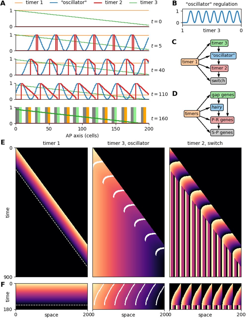
A: Simulation output at various timepoints, showing all modules. Same data as F. B: Mapping between timer 3 input state and “oscillator” output state. C,D: Comparison of model topology with the Drosophila segmentation network. P-R = pair-rule, S-P = segment-polarity. E,F: Kymographs comparing the clock and three timers model to the three timers and no clock model, using the same parameter values. Both time axes to scale. Orange = 1, black = 0. Dashed white line indicates when timer 1 reaches 0. White lines overlaid on timer 3 output (middle) mark oscillator peaks.
The final pattern is therefore governed by the dynamics of the oscillator and timer 3 in the posterior of the embryo: the oscillator generates a periodic pattern that is transduced into different segment polarity fates, and timer 3 generates a monotonic pattern that is transduced into region-specific differences. The states of these modules when the posterior signal is removed from a cell determine its ultimate fate. Thus, time is used to generate differences in o and τ3, and the system translates these into spatial patterns by TST. The mechanism is elegant, but not very efficient – the actual time that each segment is actively undergoing patterning is short, with a much longer time spent waiting around for anterior or posterior segments to undergo maturation. The process would finish much faster if segment patterning could be parallelised.
Suppose an embryo is initialised at its final length, and, in the absence of a PSC, timer 1 counts down in all cells simultaneously. Without axial elongation, spatial differences in o and τ3 are no longer generated automatically, and must be re-introduced by other means. Since the required timer 3 pattern is monotonic and the required oscillator pattern is not, it seems reasonable to assume that the timer 3 pattern is the easier to create de novo. I therefore build a montonic gradient of timer 3 state into the initial conditions, representing the early patterning of gap gene expression by maternal gradients in Drosophila [157]. To produce stripes of oscillator expression, I change the regulation of the oscillator module so that it no longer has autonomous dynamics, but instead responds to timer 3 state (Fig 3B,C). This input-output mapping represents the evolution of stripe-specific hairy enhancers regulated by gap genes [181, 211].
Simulating this model (Fig 7A, Movie 11) shows that it produces the same final output as the clock and 3 timers model, in just a fraction of the time (compare Fig 7E,F). The tissue-level dynamics are different, but the intracellular dynamics are preserved. Timer 3 gradually ticks down in each cell (albeit only through a fraction of its full dynamic range), meaning that its monotonic spatial pattern marches anteriorly across the tissue, dragging the “oscillator” pattern with it to produce spatial waves. Because these waves recapitulate the dynamical output of an intact oscillator, the stripe peaks are still able to generate temporal gradients of timer 2 expression in their wakes. Just as the timer 2 pattern is completed, timer 1 reaches its ground state, triggering the conversion of this pattern into stable segment-polarity expression.
Comparing the three timers and no clock model (Fig 7C) to the Drosophila segmentation hierarchy (Fig 7D) [1, 212] reveals that their structure is almost identical, except that the gap genes also provide considerable direct input into non-hairy pair-rule genes. In Drosophila, the pair-rule genes (timer 2) are patterned partially by stripe-specific enhancers (PI) [181] and partially by cross-regulatory dynamics (TST) [122, 123, 192], rather than purely by TST. The model could indeed be sped up even further if timer 3 additionally helped to establish timer 2, because most of the patterning time is taken up by timer 2 dynamics. Indeed, it is notable that gap gene-mediated patterning is most important for pair-rule genes expressed “earlier” in the pattern repeat (assuming a repeat stretches from one hairy stripe to the next), while cross-regulation dominates for those expressed “later”.
9 Discussion
In this article, I have used a simple modelling framework to explore the tissue-level consequences of interlinked cell-autonomous dynamical processes in the context of segmentation. I have compared the ramifications of temporal vs spatial regulation of the SAZ, considered the various spatial outputs that can be generated downstream of an oscillation, and examined the evolutionary relationship between sequential and simultaneous segment patterning. Here, I discuss the specific implications of each model, the developmental significance of TST, and the advantages and disadvantages of the “dynamical module” approach.
9.1 Temporal or spatial patterning of the SAZ?
SAZ patterning has been thought about in a number of different ways. One conceptual division concerns whether the anterior and posterior ends of the SAZ are functionally linked. In some models (usually informal), the anterior boundary of the SAZ is determined by the rate of tissue maturation, the posterior boundary of the SAZ is determined by the rate of axial elongation, and the two independent processes must be coordinated (“balanced”) to maintain an appropriate SAZ length [111, 150]. In others, the rate of axial elongation also determines the rate of tissue maturation [37, 140].
The “temporal” and “spatial” model variants I have investigated here are both of the latter type. However, the role played by elongation rate differs between them. In the spatial variant, the size of the SAZ and its maintenance over time are both independent of elongation; if elongation stops, tissue maturation stops and the SAZ remains the same size. In the temporal variant, SAZ size scales with elongation rate; if elongation stops, tissue maturation continues and the SAZ shrinks until it eventually disappears.
This difference has significant implications for segmentation dynamics, particularly when the elongation rate and/or other system parameters vary over time. Temporal patterning provides a mechanistic explanation for the scaling of SAZ size with embryo size [45] and predicts constant [42] or smoothly-varying [149] wave patterns, while spatial patterning does neither. In addition, temporal patterning is very sensitive to variation in elongation rate whereas spatial patterning buffers it; these properties could be advantages or liabilities depending on whether such variation plays instructive or destructive roles in the system. Finally, temporal patterning significantly reduces the interpretational burden of the cell (because its state trajectory can be partially autonomous), and also removes the expectation that the determination front should necessarily correspond with a particular signalling threshold [46].
The strict opposition between temporal (TST) and spatial (PI) patterning presented here is artificial; in reality, an SAZ will be patterned by both. Experiments that characterise cell state trajectories under a range of constant conditions could help quantify their relative contributions. Similar experiments combined with misexpression of (for example) Hox and gap genes would be informative about the mechanistic origins of axial variation.
9.2 From oscillations to polarisation
The problem of segment polarisation and the inadequacy of a two-state prepattern was recognised by Meinhardt even before the expression of any segment-polarity gene had been visualised [213, 214]. Here, I have demonstrated three strategies by which a sinusoidal temporal input can be used to specify a polarised spatial pattern: (1) using a timer network to calculate oscillation phase; (2) having the oscillator regulate the rate of elongation; and (3) having the oscillator regulate the rate of cell maturation.
The first strategy is consistent with, and inspired by, the cross-regulatory interactions between the pair-rule genes in Drosophila [1, 123], which likely evolved in a sequential segmentation context [92, 123, 215]. However, as yet relatively little is known about arthropod segmentation clocks and the way they regulate their downstream targets [1]. Characterising these networks in sequentially segmenting model species such as Tribolium (beetle) [14, 201], Oncopeltus (hemipteran bug) and Parasteatoda (spider) is a research priority.
A more general point illustrated by the timer strategy is that the phase relationship of linked dynamical processes will change along the SAZ if they do not share a common frequency profile. This has been discussed in the context of the vertebrate segmentation clock, which combines direct her /hes autorepression and indirect auto repression via Notch signalling. Modelling suggests that the time delays in the two feedback loops should scale similarly along the SAZ, to avoid the oscillations being extinguished [196, 216]. For other cross-regulating processes, altered phase relationships along the SAZ have been clearly documented, and the phenomenon appears to be functionally important for segment patterning [206, 217, 218].
The other two strategies involve generating a pulsatile rather than smooth progression of the wave-front, so that only certain phases of the oscillations are recorded. Rhythmic SAZ morphogenesis has been described in insects [66], where toll genes regulate convergent extension downstream of the clock [65]. In vertebrates, cell proliferation has been found to occur preferentially at the trough phase of an oscillation [148], providing another mechanism by which elongation and oscillation could be coordinated. her /hes oscillations have also been shown to delay cell differentiation in cultured cells [219], while wavefront progression appears to be modulated by the segmentation clock in zebrafish [207, 208]. Combined with the sawtooth arrest dynamics of zebrafish oscillations [197], these observations suggest that the oscillator frequency profile might play a functional role in patterning somite morphogenesis.
Finally, it is significant that the frequency profile plays an explicit role in all three of the polarisation mechanisms I have described. Progressively narrowing travelling waves (a consequence of the frequency profile) are one of the most visually striking features of segmenting systems, but in most segmentation models they lack an instructive function [37, 45, 89, 220].
9.3 From sequential to simultaneous
The final model (three timers and no clock) demonstrates the considerable dynamical and regulatory continuity between sequential and simultaneous modes of segmentation. The central idea is that regionalisation processes, ancestrally parallel to and independent of segment patterning, provided a rich source of spatial cues that could be exploited to compensate for the loss of autonomous oscillations and the SAZ framework [1, 123, 221]. Thus similar expression relationships are observed between gap genes and pair-rule genes in sequentially segmenting and simultaneously segmenting species, but stripe formation is only governed by gap inputs in the latter.
Importantly, the preservation of the regulatory machinery downstream of the “oscillator” means that the regulatory links between the regionalisation system (gap genes) and the segment patterning system (pair-rule genes) need not be extensive, so long as the ancestral gap gene expression dynamics are preserved. At minimum, the gap gene pattern need specify only the start location of each pattern repeat (white lines in Fig 7E), and cross-regulation will fill in the rest. In Drosophila, the regulatory links between the gap genes and pair-rule genes are considerably more far-reaching than this [181], and some of the presumed ancestral cross-regulation between the pair-rule genes must have been lost [123] Indeed, gene expression shifts are subtle in most of the embryo, and absent up to around the second or third pair-rule repeat [166, 188, 189]. However, expression shifts are larger and more extensive in other simultaneously segmenting species [182, 222–226], which may represent more “transitional” forms. Comparative analysis of pair-rule gene regulation in these species will be instructive.
9.4 Time-space translation in developmental systems
The central idea of TST is that spatial information can be specified by the combination of a timer and a velocity, because distance = velocity ∗ time. Many of the patterning mechanisms in this article depend on the intersection of a moving posterior signal (a velocity) with autonomous cellular processes (time). Most of the patterning burden falls on the latter, whose regulatory logic, rates, and time delays would be implicitly encoded in the sequences of enhancers, exons, and UTRs. Thus, the interaction between inherited information and a directional morphogenetic process enables a complex pattern to emerge from a simple initial state.
In the somitogenesis literature, it has sometimes been stated that the segmentation clock determines when patterning occurs, while the wavefront determines where patterning occurs [38, 111]. In reality, given that the frequency profile generates spatial waves from the oscillations, and that these may in turn feed back on the wavefront, the division of labour is not this distinct. It is more useful to think about spatial information being split between various different processes, and repeatedly redistributed between them.
The final model I present provides a particularly clear example. For one thing, the supposed temporal vs spatial roles of “clock” (oscillator) and “wavefront” (timer 1) have been reversed. More importantly, the spatial information in the system is twice converted between different forms. First, the initial spatial pattern of timer 3 combines with the temporal dynamics of timer 3 to produce posterior-to-anterior waves (distance/time = velocity). This results in waves of “oscillator” expression, which then combine with the temporal dynamics of timer 2 to produce the spatial inputs to the switch (velocity ∗ time = distance).
Thus, while there is an effective mapping between the timer 3 pattern at the beginning and the segment-polarity pattern at the end, the specific nature of the mapping depends on various dynamical rates. In Drosophila, this means that accurate and precise prediction of pair-rule gene outputs from gap gene inputs [227] is to be expected, but it need not imply that pair-rule gene regulation involves corresponding detail in signal decoding. As described in the previous section, the dynamics of patterning mean that only a subset of pair-rule stripes need to be positioned exactly, and selection on the gap gene system is likely to have adapted it specifically to this task [1].
9.5 Combining patterning strategies
In most of the models I have presented, the only intercellular signalling process is the Boolean posterior signal. The cells follow autonomous dynamical trajectories and produce coherent spatial patterns only because of their spatial ordering and temporal precision. This framework highlights the patterning capabilities of TST but is obviously incongruous with noisy, three-dimensional biology. In reality, the mechanisms presented here would be integrated with local cell communication, longer-range signalling, and morphogenetic feedback.
For example, Notch signalling-mediated self-organisation is required to counteract the oscillator desynchronisation produced by gene expression noise, division-induced expression delays, and cell rearrangement [35, 68, 228, 229]. Beyond simply preventing oscillations from deteriorating, the process also influences their period, amplitude, and frequency profile [31, 37, 118, 144, 230–234]. It will be necessary to study the interactions between self-organisation, PI, and TST mechanisms to properly understand the logic and reproducibility of developing systems.
Even the Drosophila blastoderm is a case in point. The establishment of the pattern of gap gene expression, which is impressively robust to variation in egg size and gene dosage [194, 235], seems to involve both PI and self-organisation mechanisms. The Bicoid concentration gradient is clearly instructive [236], but there is not a strict correspondence between Bicoid concentration and output gene expression to support strongly interpretational pattern formation [193, 194]. Indeed, diffusion of gene products between nuclei and cross-regulation between early gradients points to important reaction-diffusion effects [237–241]. Adding in the TST involved in segment patterning, it seems that all three patterning mechanisms are cooperating before complex morphogenesis has even begun.
9.6 The nature and evolution of dynamical modules
The “dynamical modules” of the models represent the expression dynamics of gene regulatory networks, potentially incorporating other autonomous processes such as signal decay. The focus of the models is on how different sets of dynamical processes might interact with or modulate each other, and how this could generate or transform spatiotemporal patterns.
There is an undeniable need for experimental and modelling studies that link the dynamical behaviours of networks to their topology and quantitative features [16, 62, 226, 242–246], something my study does not attempt to do. However, there are also advantages to using such a high level of abstraction. First, it focuses attention on the functional role of a dynamical behaviour, rather than its specific molecular implementation, making it easier to recognise general results. Second, a potentially complex process can be represented by a single parameter value (such as an effective timescale), rather than by a large number of regulatory interactions and rates, some of which may be experimentally inaccessible.
Beyond simple convenience, the dynamics of a process may be more conserved and/or functionally relevant than its mechanistic basis. Evolutionary systems drift [247] and local adaptation may cause the regulatory logic of homologous processes to diverge, even while their output is maintained by selection. See, for example, the differences in her /hes gene regulation across different vertebrate segmentation clocks, even though the genes’ oscillatory dynamics and down-stream functions are essentially unchanged [173, 202, 248–250]. At the same time, unrelated processes may share similar functions owing to convergent dynamics [251, 252] — different clock and wavefront systems (including arthropod segmentation and vertebrate somitogenesis) are a case in point [253, 254].
Finally, certain “modules” may be strikingly conserved across evolution, and perform intriguingly pleiotropic developmental roles. The temporal sequence of gap gene expression is seen not only in simultaneous and sequential segmentation as discussed here, but also in the patterning of neuroblasts [255–258]. Hes oscillations, too, are seen in the nervous system [259–261] and various other cellular contexts [219, 262, 263], while Hox gene dynamics are conserved across bilaterian AP axes [153, 162, 264] and reiterated in the vertebrate limb [265, 266]. Studying the origin, mechanistic basis, and evolutionary cooption/adaptation of dynamical modules is likely to provide insight into both micro- and macro-evolutionary change.
Supplementary Materials
Supplementary Document: model details.
Supplementary Movie 1: simulations corresponding to Fig 3A-D.
Supplementary Movie 2: simulations comparing temporal and spatial variants of clock and timer model.
Supplementary Movie 3: simulations corresponding to Fig 4E-H.
Supplementary Movie 4: simulations corresponding to Fig 5D,E.
Supplementary Movie 5: simulations corresponding to Fig 5D,H.
Supplementary Movie 6: simulations corresponding to Fig 6A-C.
Supplementary Movie 7: simulations corresponding to Fig 6D, temporal and spatial variants.
Supplementary Movie 8: simulations corresponding to Fig 6E, temporal and spatial variants.
Supplementary Movie 9: simulations corresponding to Fig 6F, temporal and spatial variants.
Supplementary Movie 10: simulation corresponding to Fig 6G.
Supplementary Movie 11: simulations corresponding to Fig 7A/F and Fig 7E.
Funding
This work was supported by an EMBO Postdoctoral Fellowship [EMBO ALTF 383-2018].
Acknowledgments
I thank Michael Akam, Matthew Benton, Rosa Martinez-Corral and Timothy Harden for comments on the manuscript.
Footnotes
↵* The mechanistic basis for the frequency profile is still un-clear, but seems to involve cell state dependent time delays [196]. Note that empirically characterised frequency profiles do not decrease smoothly to 0 as shown in Fig 3E [18, 115, 197], but the discrepancy is not important for my conclusions.
↵† This is known as “pair-rule” patterning, or double-segment periodicity. N.B., the “pair-rule gene” class of transcription factors are not universally expressed in pair-rule patterns, despite the name.
References
- 1.↵
- 2.↵
- 3.↵
- 4.↵
- 5.↵
- 6.↵
- 7.↵
- 8.
- 9.
- 10.↵
- 11.↵
- 12.
- 13.↵
- 14.↵
- 15.↵
- 16.↵
- 17.
- 18.↵
- 19.↵
- 20.
- 21.↵
- 22.↵
- 23.
- 24.↵
- 25.↵
- 26.↵
- 27.↵
- 28.↵
- 29.↵
- 30.↵
- 31.↵
- 32.↵
- 33.
- 34.
- 35.↵
- 36.↵
- 37.↵
- 38.↵
- 39.↵
- 40.
- 41.
- 42.↵
- 43.
- 44.↵
- 45.↵
- 46.↵
- 47.↵
- 48.↵
- 49.↵
- 50.
- 51.↵
- 52.↵
- 53.
- 54.↵
- 55.↵
- 56.↵
- 57.
- 58.
- 59.↵
- 60.↵
- 61.↵
- 62.↵
- 63.↵
- 64.
- 65.↵
- 66.↵
- 67.↵
- 68.↵
- 69.
- 70.
- 71.↵
- 72.
- 73.↵
- 74.↵
- 75.
- 76.
- 77.↵
- 78.
- 79.
- 80.
- 81.
- 82.
- 83.
- 84.↵
- 85.↵
- 86.↵
- 87.↵
- 88.↵
- 89.↵
- 90.
- 91.
- 92.↵
- 93.
- 94.↵
- 95.↵
- 96.
- 97.↵
- 98.↵
- 99.
- 100.↵
- 101.↵
- 102.
- 103.↵
- 104.↵
- 105.↵
- 106.↵
- 107.↵
- 108.↵
- 109.↵
- 110.↵
- 111.↵
- 112.
- 113.↵
- 114.↵
- 115.↵
- 116.↵
- 117.↵
- 118.↵
- 119.↵
- 120.
- 121.
- 122.↵
- 123.↵
- 124.↵
- 125.
- 126.
- 127.↵
- 128.↵
- 129.↵
- 130.↵
- 131.
- 132.↵
- 133.↵
- 134.↵
- 135.↵
- 136.↵
- 137.↵
- 138.
- 139.
- 140.↵
- 141.
- 142.↵
- 143.
- 144.↵
- 145.
- 146.
- 147.↵
- 148.↵
- 149.↵
- 150.↵
- 151.↵
- 152.
- 153.↵
- 154.
- 155.↵
- 156.↵
- 157.↵
- 158.↵
- 159.
- 160.↵
- 161.↵
- 162.↵
- 163.
- 164.↵
- 165.↵
- 166.↵
- 167.↵
- 168.↵
- 169.
- 170.↵
- 171.↵
- 172.↵
- 173.↵
- 174.↵
- 175.↵
- 176.↵
- 177.↵
- 178.↵
- 179.
- 180.
- 181.↵
- 182.↵
- 183.↵
- 184.↵
- 185.↵
- 186.↵
- 187.↵
- 188.↵
- 189.↵
- 190.
- 191.↵
- 192.↵
- 193.↵
- 194.↵
- 195.↵
- 196.↵
- 197.↵
- 198.↵
- 199.↵
- 200.↵
- 201.↵
- 202.↵
- 203.↵
- 204.↵
- 205.↵
- 206.↵
- 207.↵
- 208.↵
- 209.
- 210.↵
- 211.↵
- 212.↵
- 213.↵
- 214.↵
- 215.↵
- 216.↵
- 217.↵
- 218.↵
- 219.↵
- 220.↵
- 221.↵
- 222.↵
- 223.
- 224.
- 225.
- 226.↵
- 227.↵
- 228.↵
- 229.↵
- 230.↵
- 231.
- 232.
- 233.
- 234.↵
- 235.↵
- 236.↵
- 237.↵
- 238.
- 239.
- 240.
- 241.↵
- 242.↵
- 243.
- 244.
- 245.
- 246.↵
- 247.↵
- 248.↵
- 249.
- 250.↵
- 251.↵
- 252.↵
- 253.↵
- 254.↵
- 255.↵
- 256.
- 257.
- 258.↵
- 259.↵
- 260.
- 261.↵
- 262.↵
- 263.↵
- 264.↵
- 265.↵
- 266.↵


