Unpredictability vs. volatility and the control of learning

Abstract

Influential research has stressed the importance of uncertainty for controlling the speed of learning, and of volatility (the inferred rate of change) in this process. This framework recasts biological learning as a problem of statistical inference, to produce prominent computational models that have extensive correlates in brain and behavior and burgeoning applications to psychopathology. Here, we investigate a neglected feature of these models, which is that learning rates are jointly determined by the comparison between volatility and a second factor, unpredictability (reflecting moment-to-moment stochasticity rather than systematic change). For the organism, volatility and unpredictability both manifest as noisy experiences, but for learning, they should have opposite effects: learning should speed up as volatility increases but slow down as unpredictability increases. Like volatility, unpredictability can vary and must be estimated by the learner. Previous work has focused on half this picture, studying how organisms estimate volatility while unpredictability is assumed fixed and known. The question how the brain estimates unpredictability (and ultimately, a full account of volatility, uncertainty and learning rates, which all depend on it) remains unaddressed. We introduce a new learning model, in which both unpredictability and volatility are learned from experience. We show evidence from the behavioral and decision neuroscience literatures that the brain distinguishes these two similar types of noise, so as to produce seemingly contradictory behavior in different situations. Further, the model highlights the extent to which inferences about volatility and unpredictability are interdependent, such that disruptions of computations related to volatility can impact computations related to unpredictability, and vice versa. We argue that this interdependence is apparent in learning following amygdala damage, and may have important implications for ongoing attempts to connect volatility and uncertainty to psychopathology.

Introduction

Among the successes of computational neuroscience is a level-spanning account of learning and conditioning, which has grounded biological plasticity mechanisms (specifically, error-driven updating) in terms of a normative analysis of the problem faced by the organism (Courville et al., 2006; Daunizeau et al., 2010; Dayan and Long, 1998; Dayan et al., 2000; Gershman et al., 2010). These models recast learning as statistical inference: using experience to estimate the amount of some outcome (e.g., food) expected on average following some cue or action. This is an important subproblem of reinforcement learning, which uses such value estimates to guide choice. The statistical framing has motivated an influential program of investigating the brain’s mechanisms for tracking uncertainty about its beliefs, and how these impact learning (Behrens et al., 2007; Iglesias et al., 2013; McGuire et al., 2014; Nassar et al., 2012; Soltani and Izquierdo, 2019). This program has shed particularly light on the principles governing the rate of learning at each step – that is, the degree one should update one’s beliefs in light of each new outcome. The statistical analysis implies that the learning rate, like all Bayesian cue combination problems, should depend on how uncertain those (prior) beliefs were balanced against the statistical noisiness of the new evidence (the likelihood). Previous work has focused on the role of the prior uncertainty in this learning rate control. In this article, we focus attention on the second, relatively neglected half of this comparison, to ask how organisms assess the noisiness of outcomes, which we call unpredictability, during learning.

The connection between uncertainty and learning rate has inspired an influential series of hierarchical Bayesian inference models, elaborating a baseline model known as the Kalman filter (Behrens et al., 2007; Mathys et al., 2011; Piray and Daw, 2020). A key feature of these models is that learning occurs over multiple trials, so the updated posterior at one step becomes the prior at the next – with the important additional twist that uncertainty increases at each step due to the possibility that the true value has changed. The hierarchical models extend the Kalman filter to also estimate the rate of such change, called volatility. All else equal, when volatility is higher, the organism is more uncertain about the cue’s value (because the true value will on average have fluctuated more following each observation), and so the learning rate (the reliance on each new outcome) should be higher. A series of experiments have reported behavioral and neural signatures of these volatility effects, and also their disruption in relation to psychiatric symptoms (Behrens et al., 2007; Brazil et al., 2017; Browning et al., 2015; Cole et al., 2020; Deserno et al., 2020; Diaconescu et al., 2020; Farashahi et al., 2017; Iglesias et al., 2013; Katthagen et al., 2018; Lawson et al., 2017; Paliwal et al., 2019; Piray et al., 2019; Powers et al., 2017; Soltani and Izquierdo, 2019). However, volatility is only one of two noise parameters in the underlying Kalman filter; the second is unpredictability, which controls how noisy are each of the outcomes (the width of the likelihood) individually. This type of noise also affects the learning rate, but in the opposite direction: all else equal, when individual outcomes are more unpredictable, they are less informative about the cue’s true value and the learning rate, in turn, should be smaller.

Although unpredictability therefore plays an equally important and symmetric role as does volatility, the line of research that extends the Kalman filter hierarchically to investigate how organisms estimate volatility has simply assumed that unpredictability is fixed and known. Accordingly, the potential effects of unpredictability on learning and choice have been largely overlooked, and the question how the brain estimates unpredictability (and thus also volatility and uncertainty, which in the general case depend on it) remains unaddressed. In this study, we fill this gap by developing a hierarchical model that simultaneously infers both quantities during learning. We then study its behavior in reinforcement learning tasks and its relationship to previous studies.

The model sheds new light on experimental phenomena of learning rates in conditioning, and on two classic descriptive theories of conditioning in psychology that have been interpreted as predecessors of the statistical accounts. The theories of Mackintosh (Mackintosh, 1975) vs Pearce and Hall (Pearce and Hall, 1980) claim in apparent contradiction that animals pay, respectively, either more or less attention to cues that are more reliably predictive of outcomes. Although these two theories are described loosely in terms of “attention,” one of the key operational counterparts of such attention (and the one relevant to the current theory) is faster learning about those cues. Indeed, different experimental procedures seem to produce either faster or slower learning when outcomes are noisier, supporting either theory. This has led to long-lasting discussions and further descriptive models of attention hybridizing the two theories (Le Pelley, 2004; Le Pelley et al., 2016; Pearce and Mackintosh, 2010). Previous work with the statistical models has also proposed to resolve this conundrum by identifying the theories with different aspects of the broad term “attention,” and in particular by arguing that Mackintosh’s logic (less attention to poor predictors) applies not to learning rates but instead when making predictions on the basis of multiple, competing cues (Dayan et al., 2000). Here, motivated by the work on volatility, we focus strictly on learning rates for a single cue or action. In this case, we argue, seemingly contradictory Mackintosh-vs. Pearce-Hall-type effects (slower or faster learning under noise) can be explained by learning rate modulation due to inferred unpredictability vs. volatility, respectively. On this view, different effects will dominate in different experiments depending on which parameter the pattern of the noise suggests.

Indeed, a core question raised by our analysis is how the brain manages to distinguish volatility from unpredictability, and when it might confuse them. Although the learner’s estimates of them play opposite roles in learning – and thus, telling them apart is crucial to appropriately control learning – from the learner’s perspective, they both similarly manifest in noisier, less reliably predictable outcomes. Dissociating them is possible, because they have distinguishable effects on the more detailed temporal pattern of the noise, specifically the residual autocorrelation in the outcomes (covariation on consecutive trials). While unpredictability decreases autocorrelation, volatility increases it. Because this difference plays out over multiple trials, detecting it poses a challenge for many approximate inference techniques, which rely on simplifying the relationship between different observables. Our model instead tackles this using a sampling-based approximation. Finally, several novel implications of this analysis arise from the fact that observed noise can, to a first approximation, be explained by either volatility or unpredictability. This means that previous work apparently showing variation in volatility processing in different groups, such as patients (using a model and tasks that do not vary unpredictability), might instead reflect misidentified abnormalities in processing unpredictability. Relatedly, from the perspective of the learner inferring these two parameters, they should compete or trade off against one another to best capture observed noise, a phenomenon known as “explaining away” in Bayesian probability theory. This means that any dysfunction or damage that impairs detection of volatility, should lead to a compensatory increase in inferred unpredictability, and vice versa. We argue that this effect can be appreciated in studies of the amygdala’s role in modulating learning rates, suggesting it is specifically tied to detecting volatility rather than learning rate more broadly. The same sorts of reciprocal interactions also give rise to a richer and subtler set of possible patterns of dysfunction that may help to constrain ongoing attempts to identify symptoms of psychopathology, such as anxiety and schizophrenia, with altered processing of uncertainty.

Results

Model

We begin with the Kalman filter, which describes statistically optimal learning from data produced according to a specific form of noisy generation process. The model assumes that the agent must draw inferences (e.g., about true reward rates) from observations (individual reward amounts) that are corrupted by two distinct sources of noise: process noise or volatility and outcome noise or unpredictability (Figure 1ab). Volatility captures the speed by which the true value being estimated changes from trial to trial (modeled as Gaussian diffusion); unpredictability describes additional measurement noise in the observation of each outcome around its true value (modeled as Gaussian noise on each trial).

Figure 1.

Statistical difference between volatility and unpredictability. a-b) Examples of generated time-series based on a small and large constant volatility parameter given a small (a) or a large (b) constant unpredictability parameter are plotted. c) Given a surprising observation (e.g. a negative outcome), one should compute how likely the outcome is due to the unpredictability (left balloon) or due to the volatility (right balloon). Dissociating these two terms is important for learning, because they have opposite influences on learning rate. d) Structure of the (generative) model: outcomes were stochastically generated based on a probabilistic model depending on reward rate, unpredictability and volatility. Only outcomes were observable (the gray circle), and value of all other parameters should be inferred based on outcomes. The observed outcome is given by the true reward rate, x_t, plus some noise whose variance is given by the true unpredictability, u_t. The reward rate itself depends on its value on the previous trial plus some noise whose variance is given by the true volatility, v_t. Both volatility and unpredictability are dynamic and probabilistic Markovian variables generated by their value on the previous trial multiplied by some independent noise. The multiplicative noise ensures that these variables are positive on every trial. See Methods for the details of the model. e-f) It is possible to infer both volatility and unpredictability based on observed outcomes, because these parameters have dissociable statistical signatures. In particular, although both of them increase variance (e), but they have opposite effects on autocorrelation (f). In particular, whereas volatility increases autocorrelation, unpredictability tends to reduce it. Here, 1-step autocorrelation (i.e. correlation between trial t and t − 1) was computed for 100 time-series generated with parameters defined in b and c. Error-bars are standard error of the mean. Small and large parameters for volatility were 0.1 and 0.4 and for unpredictability were 1 and 4, respectively.

For this data generating process, if the true values (i.e., variances) of volatility and unpredictability, v_t and u_t are known, then optimal inference about the underlying reward rate is tractable using a specific application of Bayes rule, here called the Kalman filter (Kalman, 1960). The Kalman filter represents its beliefs about the reward rate at each step as a Gaussian distribution with a mean, m_t, and variance (i.e., uncertainty about the true value), w_t. The update, on every trial, is driven by a prediction error signal, δ_t, and learning rate, α_t. This leads to simple update rules following observation of outcome o_t: This derivation thus provides a rationale for the error-driven update prominent in neuroscience and psychology (Kakade and Dayan, 2002), and adds to these a principled account of the learning rate, α_t, which on this view should depend (Eq. 2) on the agent’s uncertainty and the noise characteristics of the environment. In particular, Eq. 2 shows that the learning rate is increasing and decreasing, respectively, with volatility and unpredictability. This is because higher volatility increases the chance that the true value will have changed since last observed (increasing the need to rely on the new observation), but higher unpredictability decreases the informativeness of the new observation relative to previous beliefs.

This observation launched a line of research focused on elucidating and testing the prediction that organisms adopt higher learning rates when volatility is higher (Behrens et al., 2007). But the very premise of these experiments violates the simplifying assumption of the Kalman filter – that volatility is fixed and known to the agent. To handle this situation, new models were developed (Mathys et al., 2011; Piray and Daw, 2020) that generalize the Kalman filter to incorporate learning the volatility v_t as well, arising from Bayesian inference in a hierarchical generative model in which the true v_t is also changing. In this case, exact inference is no longer tractable, but approximate inference is possible and typically incorporates Eqs. 1-4 as a subprocess.

This line of work on volatility estimation inherited from the Kalman filter the view of unpredictability as fixed and known. The premise of the current article is that all the same considerations apply to unpredictability as well: it must be learned from experience, may be changing, and its value impacts learning rate. Indeed, learning both parameters is critical for efficient learning, because they have opposite effects on learning rate: whereas volatility increases the learning rate, unpredictability reduces it (Figure 1c).

Learning these two parameters simultaneously is difficult because, from the perspective of the agent, larger values of either volatility or unpredictability result in more surprising observations: i.e., larger outcome variance (Figure 1e). However, there is a subtle and critical difference between the effects of these parameters on generated outcomes: whereas larger volatility increases the autocorrelation between outcomes (i.e. covariation between outcomes on consecutive trials), unpredictability reduces the autocorrelation (Figure 1f). This is the key point that makes it possible to dissociate and infer these two terms while only observing outcomes.

We developed a probabilistic model for learning under these circumstances. The data generation process arises from a further hierarchical generalization of these models (especially the generative model used in our recent work (Piray and Daw, 2020)), in which the true value of unpredictability u_t is unknown and changing, as are the true reward rate and volatility (Figure 1d). The goal of the learner is to estimate the true reward rate from observations, which necessitates inferring volatility and unpredictability as well.

As with models of volatility, exact inference for this generative process is intractable. Furthermore, this problem is also challenging to handle with variational inference, the family of approximate inference techniques used previously (see Discussion). Thus, we have instead used a different standard approximation approach that has also been popular in psychology and neuroscience, Monte Carlo sampling (Brown and Steyvers, 2009; Courville et al., 2006; Daw and Courville, 2008; Griffiths et al., 2006). In particular, we use particle filtering to track v_t and u_t based on data (Doucet and Johansen, 2011; Doucet et al., 2000). Our method exploits the fact that given a sample of volatility and unpredictability, inference for the reward rate is tractable and is given by Eqs 1-4, in which u_t and v_t are replaced by their corresponding samples (see Methods).

Learning under volatility and unpredictability

We now consider the implications of this model for learning under volatility and unpredictability.

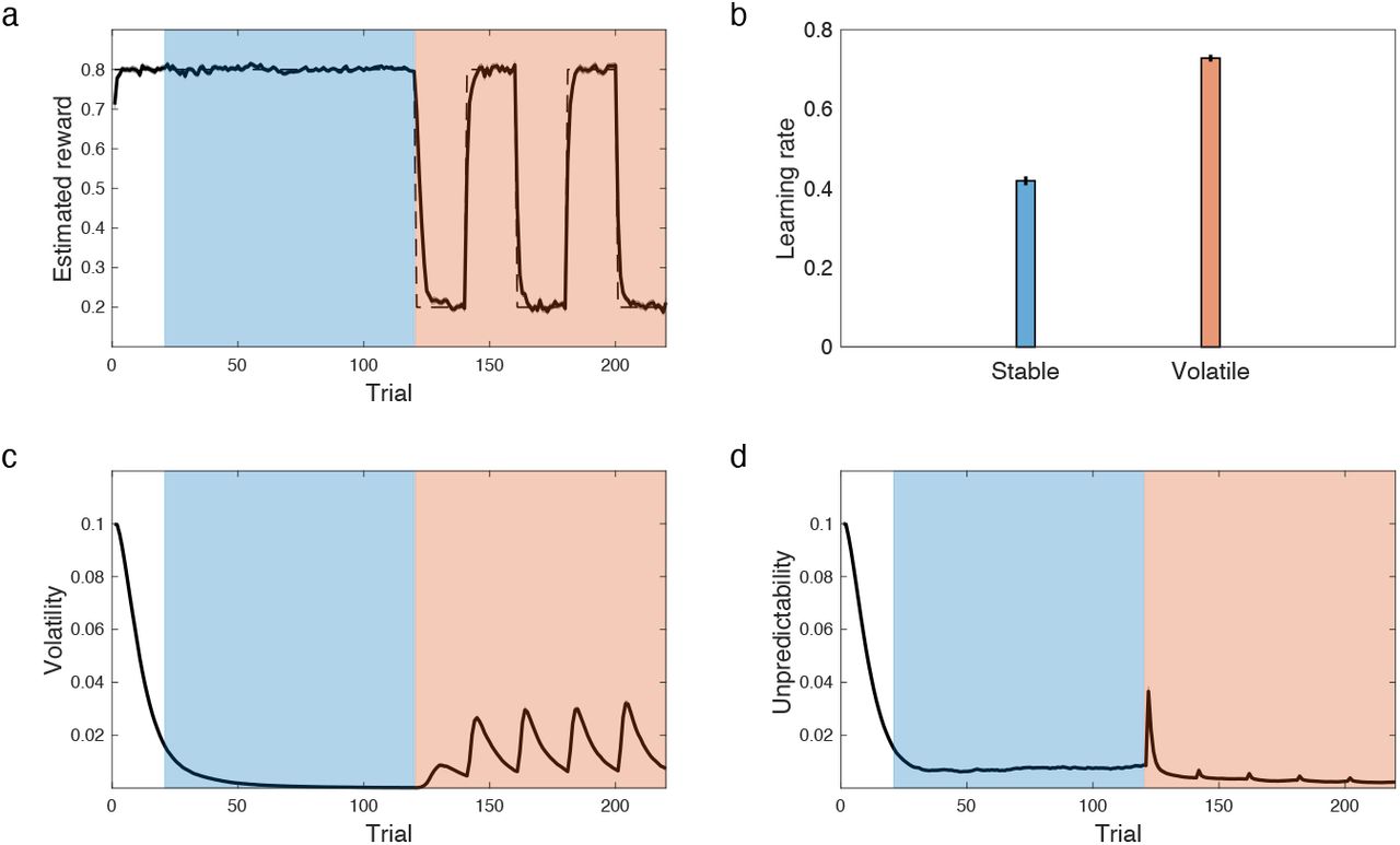
A series of studies has used two-level manipulations (high vs low volatility blockwise) to investigate the prediction that learning rates should increase under high volatility (Behrens et al., 2007, 2008; Browning et al., 2015; Pulcu and Browning, 2017). Here volatility has been operationalized by frequent or infrequent reversals (Figure 2a), rather than the smoother Gaussian diffusion that the volatility-augmented Kalman filter models formally assume. Nevertheless, applied to this type of task, these models detect higher volatility in the frequent-reversal blocks, and increase their learning rates accordingly (Behrens et al., 2007; Mathys et al., 2011; Piray and Daw, 2020). The current model (which effectively incorporates the others as a special case) achieves the same result (Figure 2).

Figure 2.

The model elevates its learning rate in volatile environments. a) Simulations of our model in the volatility learning paradigm, in which subjects undergo stable (bluish) and volatile blocks (orangish) of learning. Dashed and solid line show true reward and estimated reward by the model, respectively. b) learning rate is larger in the volatile block compared with the stable one, similar to those reported in humans. This is because the volatility term (c) increases more than the unpredictability term (d) in the volatile condition. Errorbars reflect standard error of the mean over 100 simulations and are, for some parameters, too small to be visible.

We next consider a variant of this type of task, elaborated to include a 2×2 factorial manipulation of both unpredictability alongside volatility (Figure 3; we also substitute smooth diffusion for reversals). Here both parameters are constant within the task, but they are unknown to the model. A series of outcomes was generated based on a Markov random walk in which the hidden reward rate is changing according to a random walk and the learner observes outcomes that are noisily generated according to the reward rate.

Figure 3.

Performance of the model in task with constant but unknown volatility and unpredictability parameters. a) Learning rate in the model varies by changes in both the true volatility and unpredictability. Furthermore, these parameters have opposite effects on learning rate. In contrast to volatility, higher unpredictability reduces the learning rate. b) Estimated volatility captures variations in true volatility (small: 0.5; large: 1.5). c) Estimated unpredictability captures variations in the true unpredictability (small: 2; large: 6). In (a-c), average learning rate, estimated volatility and unpredictability in the last 20 trials were plotted over all simulations (100 simulations). d-f) Learning rate, volatility and unpredictability estimates by the model for small true unpredictability. g-i) The three signals are plotted for the larger true unpredictability. Estimated volatility and unpredictability by the model capture their corresponding true values. In panels a-c, mean over the last 10 trials of each task has been plotted. Error bars reflect standard error of the mean over 100 simulations.

Figure 3 shows the model’s learning rates and how these follow from its inferences of volatility and unpredictability. As above, the model increases its learning rate in the higher volatility conditions; but as expected it also decreases it in the higher unpredictability conditions (Figure 3a). These effects on learning rate arise, in turn (via Eq. 2) because the model is able to correctly estimate the various combinations of volatility and unpredictability from the data (Figure 3bc).

Our model thus suggests a general program of augmenting the standard 2-level volatility manipulation to include a second manipulation, of unpredictability, and makes the novel prediction that higher unpredictability should decrease learning rate, separate from volatility effects. To our knowledge, unpredictability has largely not yet been manipulated in studies of learning in human decision neuroscience (see Discussion for a few exceptions); Analogous effects of unpredictability effects have been seen in another line of studies (Nassar et al., 2010, 2012, 2016), but to our knowledge, unpredictability has largely not yet been manipulated alongside volatility in studies of learning in human decision neuroscience. Thus we next consider related evidence from animal conditioning. In particular, we suggest, the predicted effects of unpredictability and volatility relate to two distinct lines of theory and data from this literature.

Unpredictability vs. volatility in Pavlovian learning

Learning rates and their dependence upon previous experience have been more extensively studied in Pavlovian conditioning. In this respect, a distinction emerges between two seemingly contradictory lines of theory and experiment, those of Mackintosh (1975) vs Pearce and Hall (1980). Both of these theories concern how the history of experiences with some cue drives animals to devote more or less “attention” to it. Attention is envisioned to affect several phenomena including not just rates of learning about the cue, but also other aspects of their processing, such as competition between multiple stimuli presented in compound. Here, to most clearly examine the relationship with the research and models discussed above, we focus specifically on learning rates for a single cue.

The two lines of models start with opposing core intuitions. Mackintosh (1975) argues that animals should pay more attention to (e.g., learn faster about) cues that have in the past been more reliable predictors of outcomes. Pearce and Hall (1980) argue for the opposite: faster learning about cues that have previously been accompanied by surprising outcomes, i.e. those that have been less reliably predictive.

Indeed, different experiments – as discussed below – support either view. For our purposes, we can view these experiments as involving two phases: a pretraining phase that manipulates unpredictability or surprise, followed by a retraining phase to test how this affects the speed of subsequent (re)learning. In terms of our model, we can interpret the pretraining phase as establishing inferences about unpredictability and volatility, which then (depending on their balance) govern learning rate during retraining. On this view, noisier pretraining might, depending on the pattern of noise, lead to either higher volatility and higher learning rates (consistent with Pearce-Hall) or higher unpredictability and lower learning rates (consistent with Mackintosh).

First consider volatility. It has been argued that the Pearce-Hall (1980) logic is formalized by volatility-learning models (Courville et al., 2006; Dayan et al., 2000; Piray and Daw, 2020). In these models, surprising outcomes during pretraining increase inferred volatility and thus speed subsequent relearning. Hall and Pearce (Hall and Pearce, 1982; Pearce and Hall, 1980) pretrained rats with a tone stimulus predicting a moderate shock. In the retraining phase, the intensity of the shock was increased. Critically, one group of rats experienced a few surprising “omission” trials at the end of the pretraining phase, in which the tone stimulus was presented with no shock. The speed of learning was substantially increased following the omission trials compared with a control group that experienced no omission in pretraining. Figure 4 shows a simulation of this experiment from the current model, showing that the omission trials lead to increased volatility and faster learning. Note that the history-dependence of learning rates in this type of experiment also rejects simpler models like the Kalman filter, in which volatility (and unpredictability) are taken as fixed; for the Kalman filter, learning rate depends only on the number of pretraining trials but not the particular pattern of observed outcomes.

Figure 4.

The model explains Pearce and Hall’s conditioned suppression experiment. a) The design of experiment (Hall and Pearce, 1982), in which they found that the omission group show higher speed of learning than the control group. b) Median learning rate over the first trial of the retraining. The learning rate is larger for the omission group due to increases of volatility (c), while unpredictability is similar for both groups. Errorbars reflect standard error of the median over 100 simulations.

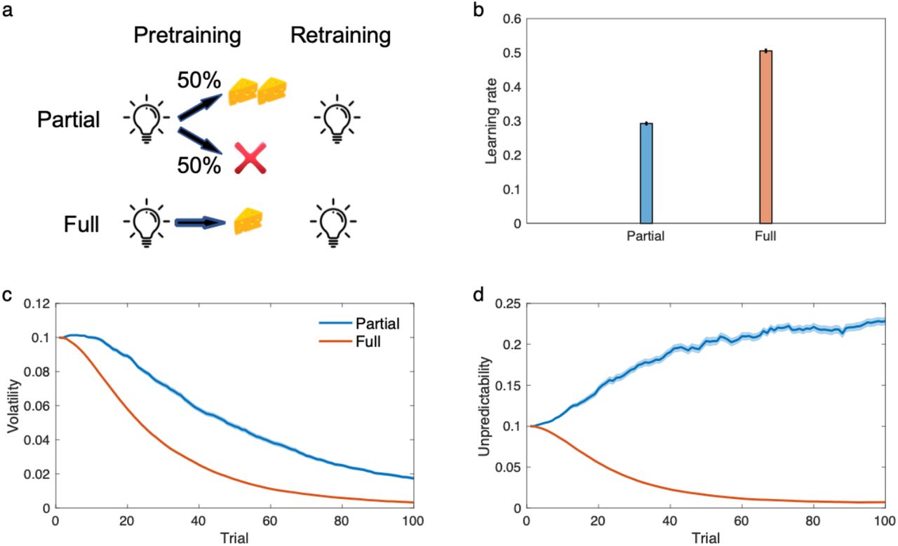
Next, consider unpredictability. Perhaps the best example of Mackintosh’s (1975) principle in terms of learning rates for a single cue is the “partial reinforcement extinction effect” (Gibbon et al., 1980; Haselgrove et al., 2004; Rescorla, 1999). Here, for pretraining, a cue is reinforced either on every trial or instead (“partial reinforcement”) on only a fraction of trials. The number of times that the learner encounters the stimulus is the same for both conditions, but the outcome is noisier for the partially reinforced stimulus. The retraining phase consists of extinction (i.e. fully unreinforced presentations of the cue), which occurs faster for fully reinforced cues even though they had been paired with more reinforcers initially. Our model explains this finding (Figure 5), because it infers larger unpredictability in the partially reinforced condition, leading to slower learning. Notably, this type of finding cannot be explained by models like which learn only about volatility (Behrens et al., 2007; Mathys et al., 2011; Piray and Daw, 2020). In general, this class of models mistake partial reinforcement for increased volatility (rather than increased unpredictability), and incorrectly predict faster learning.

Figure 5.

The model explains partial reinforcement extinction effects. a) The experiment consists of a partial condition in which a light cue if followed by reward on 50% of trials and a full condition in which the cue is always followed by the reward. b) Learning rate over the first trial of retraining has been plotted. Similar to empirical data, the model predicts that the learning rate is larger in the full condition, because partial reinforcements have relatively small effects on volatility (c), but it considerably increases unpredictability. Errorbars reflect standard error of the mean over 100 simulations and are, for some parameters, too small to be visible.

Note the subtle difference between the experiments of Figures 4 and 5. The surprising omission experiment involves stable pretraining prior to omission, then an abrupt shift, whereas pretraining in the partial reinforcement experiment is stochastic, but uniformly so. Accordingly, though both pretraining phases involve increased noise (relative to their controls) the model interprets the pattern of this noise as more likely reflecting either volatility or unpredictability, respectively, with opposite effects on learning rate. Overall, then, these experiments support the current model’s suggestion that organisms learn about unpredictability in addition to volatility. Conversely, the models help to clarify and reconcile the seemingly opposing theory and experiments of Mackintosh and Pearce-Hall, at least with respect to learning rates for individual cues. Indeed, although previous work has noted the relationship between Pearce-Hall surprise, uncertainty, and learning rates (Behrens et al., 2007; Dayan et al., 2000; Li et al., 2011; Piray and Daw, 2020; Piray et al., 2019), the current modeling significantly clarifies this mapping by identifying it more specifically with volatility, as contrasted against simultaneous inference about unpredictability. Relatedly, previous work attempting to map Mackintosh’s (1975) principle onto statistical models has focused on cue combination rather than learning rates (Dayan et al., 2000), which is a complementary but separate idea.

Interactions between volatility and unpredictability

The previous results highlight an important implication of the current model: that inferences about volatility and unpredictability are mutually interdependent. From the learner’s perspective, both volatility and unpredictability increase the noisiness of observations, and disentangling their respective contributions requires trading off two opposing explanations for the pattern of observations, a process known in Bayesian probability theory as explaning away. Thus, as in the experiment of Figure 5, models that neglect unpredictability tend to misidentify unpredictability as volatility and inappropriately modulate learning. Intriguingly, this situation might in principle arise in the laboratory, if some type of manipulation or damage selectively impacts inference about volatility or unpredictability. In that case, the model predicts a characteristic pattern of compensation, whereby learning rate modulation is not merely impaired but reversed, reflecting the substitution of volatility for unpredictability or vice versa: a failure of explaining away.

Such a pattern is evidently visible in the effects of amygdala damage on learning. The amygdala is known to be critical for associative learning (Averbeck and Costa, 2017; Phelps et al., 2014). Based on evidence from human neuroimaging work, single-cell recording in nonhuman primates and lesion studies in rats, different authors have proposed that the amygdala is involved in controlling learning rates (Averbeck and Costa, 2017; Costa et al., 2016; Holland and Gallagher, 1999; Homan et al., 2019; Li et al., 2011; Roesch et al., 2012).

Most informative from the perspective of our model are lesion studies in rats (Holland and Gallagher, 1993, 1999) that support an involvement specifically in processing of volatility, rather than learning rates or uncertainty more generally. These experiments examine a surprise-induced upshift in learning rate similar to the Pearce-Hall experiment from Figure 5. Lesions to the central nucleus of the amygdala attenuate this effect, suggesting a role in volatility processing. But in fact, the effect is not merely attenuated but reversed, consistent with our theory’s predictions in which volatility trades off against a (presumably anatomically separate) system for unpredictability estimation.

Figure 6 shows their serial prediction task and results in more detail. Rats performed a prediction task in two phases. A group of rats in the ‘consistent’ condition performed the same prediction task in both phases. The ‘shift’ group, in contrast, experienced a sudden change in the contingency in the second phase. Whereas the control rats showed elevation of learning rate in the shift condition manifested by elevation of food seeking behavior in the very first trial of the test, the amygdala lesioned rats showed the opposite pattern. Lesioned rats showed significantly smaller learning rate in the shift condition compared with the consistent one: a reversal of the surprise-induced upshift.

Figure 6.

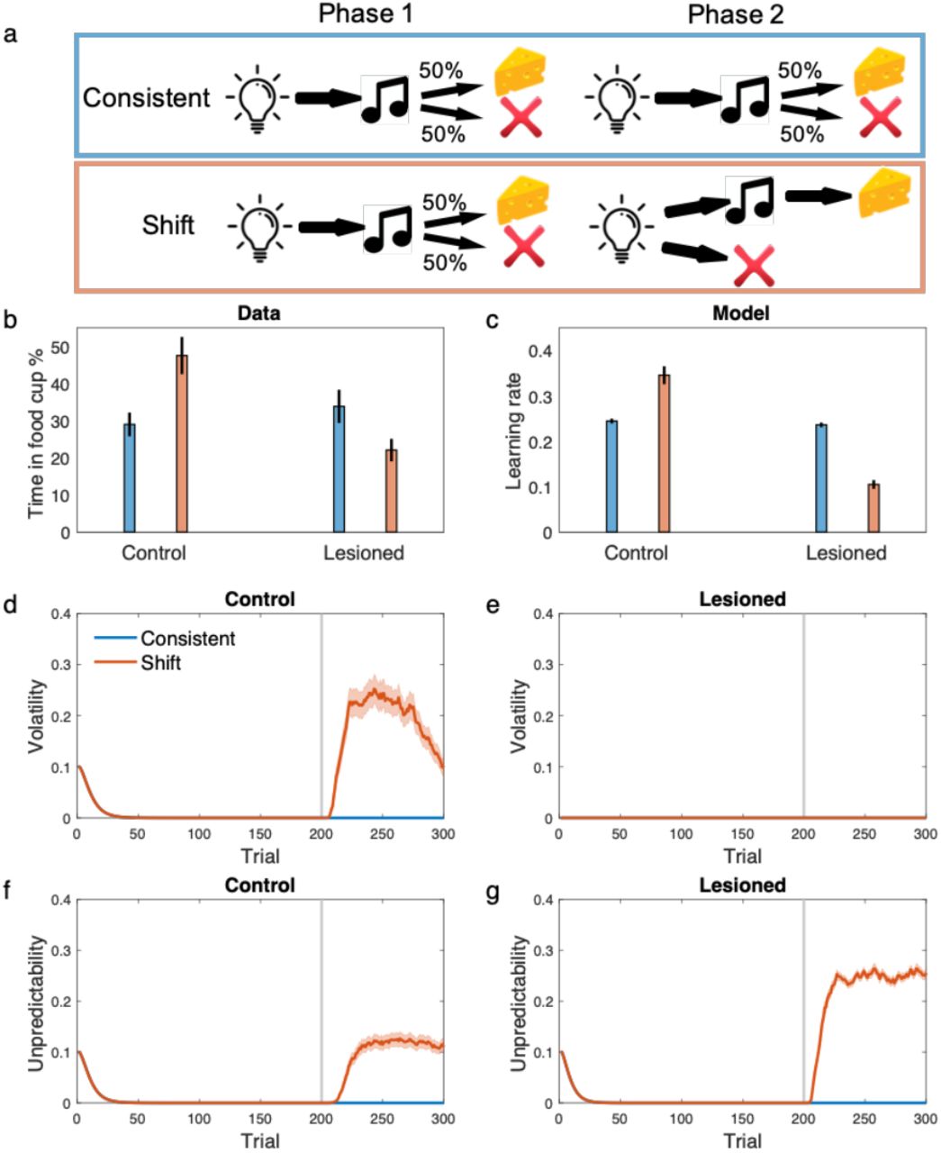
The model displays the behavior of amygdala lesioned rats in associative learning. a) The task used for studying the role of amygdala in learning by Holland and Galagher. Rats in the ‘consistent’ condition received extensive exposure to a consistent light–tone in a partial reinforcement schedule (i.e. only half of trials led to reward). In the ‘shift’ condition, however, rats were trained on the same light-tone partial reinforcement schedule in the first phase, but the schedule shifted to a different one in the shorter second phase, in which rats received light-tone-reward on half of trials and light-nothing on the other half. b) Empirical data showed that while the contingency shift facilitates learning in the control rats, it disrupts performance in lesioned rats. c) learning rate in the last trial of second phase shows the same pattern. This is because the shift increases volatility for the control rats (d) but not for the lesioned rate (e). In contrast, the contingency shift increases the unpredictability for the lesioned rats substantially more than that for the control rats, which results in reduced learning rate for the lesioned animals (f-g). The gray line shows the starting trial of the second phase. Data in (b) was original reported in (Holland and Gallagher, 1993) and reproduced here from (Holland and Schiffino, 2016). Errorbars reflect standard error of the mean over 100 simulations.

We simulated the model in this experiment. To model a hypothetical effect of amygdala lesion on volatility inference, we assumed that lesioned rats treat volatility as small and constant. As shown in Figure 6, the model shows an elevated learning rate in the shift condition for the control rats, which is again due to increases in inferred volatility after the contingency shift. For the lesioned model, however, surprise is misattributed to the unpredictability term as an increase in inferred volatility cannot explain away surprising observations (because it was held fixed). Therefore, the contingency shift inevitably increases unpredictability and thereby decreases the learning rate. Notably, the compensatory reversal in this experiment cannot be explained using models that do not consider both volatility and unpredictability terms.

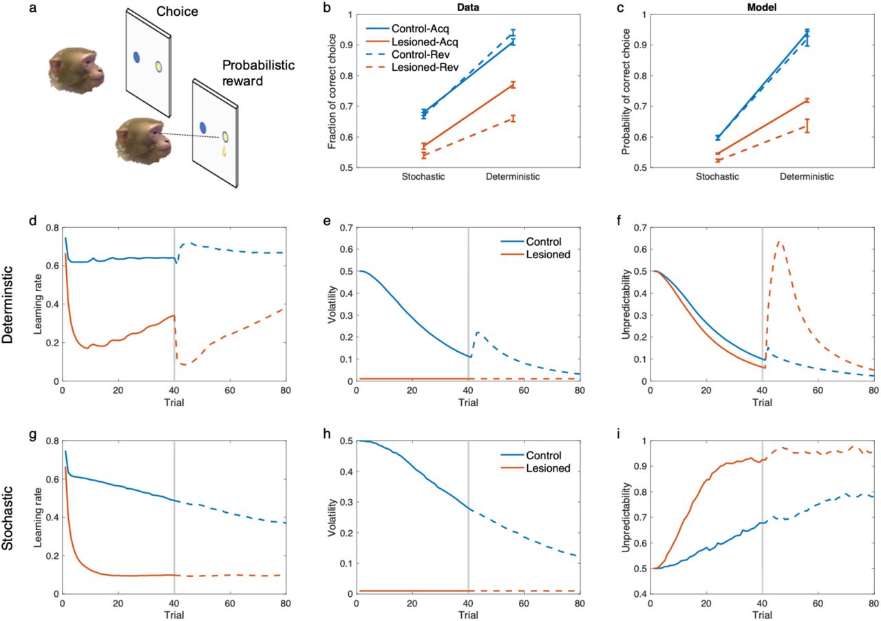
A similar pattern of effects of amygdala lesions, consistent with our theory, is seen in an experiment on non-human primates (Figure 7). In a recent report by Costa et al. (2016), it has been found that amygdala lesions in monkeys disrupt reversal learning with deterministic contingencies, moreso than a reversal task with stochastic contingencies. This is even though deterministic reversal learning tasks are much easier. Similar to the previous experiment, our model explains this finding because large surprises caused by the contingency reversal are misattributed to the unpredictability in lesioned animals (because volatility was held fixed), while control animals correctly attribute them to the volatility term. This effect is particularly large in the deterministic case because the environment is very predictable before the reversal and therefore the reversal causes larger surprises than those for the stochastic one. Similar findings have been found in a study in human subjects with focal bilateral amygdala lesions (Hampton et al., 2007), in which patients tend to show more deficits in deterministic reversal learning than stochastic one. Again, these experimental findings are not explained by a Kalman filter or models that only consider the volatility term.

Figure 7.

The model displays the behavior of amygdala lesioned monkeys in probabilistic reversal learning. a) The probabilistic reversal learning task by Costa et al. (2016). The task consists of 80 trials, in which animals chose one of the two stimuli by making a saccade to it and fixating on the chosen cue. A probabilistic reward was given following a correct choice. The stimulus-reward contingency was reversed in the middle of the task (on a random trial between trials 30-50). The task consists of different schedules, but we focus here on 60%/40% (stochastic) and 100%/0% (deterministic), which show the clearest difference in empirical data. b) Performance of animals in this task. In addition tothe general reduced performance by the lesioned animals, their performance was substantially more disrupted in the deterministic-than stochastic-reversal. c) Performance of the model in this task shows the same pattern. d-i) Learning rate, volatility and unpredictability signals for the deterministic (d-f) and stochastic task (g-i). Solid and dashed line are related to acquisition and reversal phase, respectively. Deterministic reversal increases the learning rate in the control animals due to increases in volatility, but not in the lesioned monkeys, in which it reduces the learning rate due to the increase of the unpredictability. The reversal in the stochastic task has very small effects on these signals, because unpredictability is relatively large during both acquisition and reversal. Errorbars reflect standard error of the mean over 100 simulations.

Overall, then, these experiments support the current model’s picture of dueling influences of unpredictability and volatility. Similar compensatory patterns might be expected in other situations where volatility or unpredictability may be impaired, such as psychiatric disorders. Relatedly, the current model helps to clarify the precise role of amygdala in this type of learning, relating it specifically to volatility-mediated adjustments.

Discussion

A central question in decision neuroscience is how the brain learns from the consequences of choices given that these can be highly noisy. To do so effectively requires simultaneously learning about the characteristics of the noise, as has been studied in a prominent line of work on how the brain tracks the volatility of the environment. Here we argue that work on this topic has largely neglected a key distinction between two importantly different types of noise: volatility and unpredictability. A statistically efficient agent should behave very differently when faced with these two types of noise. Previous work has focused on the prediction that volatility should increase the learning rate, because it signals that previous observations are less likely to remain relevant (Behrens et al., 2007; Iglesias et al., 2013). But another superficially similar type of noise, unpredictability, should instead decrease the learning rate, because it signals that individual outcomes are noisy and must be averaged over time to reveal the underlying reward rate. Efficient learning requires taking both these effects into account by estimating both types of noise and adjusting learning rates accordingly. To solve this problem, we built a novel probabilistic model for learning in uncertain environments that tracks volatility and unpredictability simultaneously. Computationally, this is possible because these two types of noise have dissociable observable signatures despite having similar effects on outcome variance. In particular, whereas volatility increases outcome autocorrelation (i.e. covariation on consecutive trials), unpredictability decreases it.

Our work builds directly on a rich line of theoretical and experimental work on the relationship between volatility and learning rates (Behrens et al., 2007; de Berker et al., 2016; Browning et al., 2015; Diaconescu et al., 2014; Farashahi et al., 2017; Iglesias et al., 2013; Khorsand and Soltani, 2017). There have been numerous reports of volatility effects on healthy and disordered behavioral and neural responses, often using a two-level manipulation of volatility like that from Figure 2 (Behrens et al., 2007; Brazil et al., 2017; Browning et al., 2015; Cole et al., 2020; Deserno et al., 2020; Diaconescu et al., 2020; Farashahi et al., 2017; Iglesias et al., 2013; Katthagen et al., 2018; Lawson et al., 2017; Paliwal et al., 2019; Piray et al., 2019; Powers et al., 2017; Pulcu and Browning, 2017; Soltani and Izquierdo, 2019). Our modeling suggests that it will be informative to drill deeper into these effects by augmenting this task to cross this manipulation with unpredictability so as more clearly to differentiate these two potential contributors. For example, in tasks that manipulate (and models that consider) only volatility, it can be seen from Equations 1-4 that the timeseries of several quantities all covary together, including the estimated volatility v_t, the posterior uncertainty w_t, and the learning rate α_t. It can therefore be difficult in general to distinguish which of these variables is really driving tantalizing neural correlates related to these processes, for instance in amygdala and dorsal anterior cingulate cortex (Behrens et al., 2007; Li et al., 2011). The inclusion of unpredictability (which increases uncertainty but decreases learning rate) would help to drive these apart.

Although volatility and unpredictability play symmetric roles in the Kalman filter, one practical reason this line of experiments has elided unpredictability thus far is that it has typically used binary rather than continuous outcomes. The underlying Kalman filter-based generative models assume observed outcomes are corrupted by real-valued Gaussian noise, whose variance is the unpredictability. However, the variance of binomial outcomes is entirely determined by their mean, so even though the underlying computational models approximate the likelihood distribution with a Gaussian, there is not independent experimental control of its variance, the unpredictability. Another related set of learning tasks has used continuous outcomes (McGuire et al., 2014; Nassar et al., 2010, 2012, 2016) (McGuire et al., 2014; Nassar et al., 2012, 2016) and could provide another foundation for factorial manipulations of the sort we propose. Indeed, a number of these studies (complementary to the volatility studies) included multiple levels of unpredictability and showed learning rate effects (Diederen and Schultz, 2015; McGuire et al., 2014; Nassar et al., 2010, 2012, 2016).

Although for the reasons discussed above, there is as yet little direct evidence from human reinforcement learning studies for our model’s predictions that learners should be simultaneously sensitive to outcome unpredictability and volatility, we report related evidence from unpredictability vs. volatility manipulations in Pavlovian learning and for compensatory effects in amygdala lesions suggesting a competitive relationship between the two sources of noise. Also, the effects of unpredictability vs volatility on learning rates are actually a case of (repeated) Bayesian cue combination, where unpredictability modulates the contribution of the likelihood and volatility (the chance of change from one trial to the next) modulates the contribution of the prior. Outside the learning context, but in noisy cue combination experiments more broadly, there is substantial evidence for effects of unpredictability alongside prior variance (i.e., the variance of the likelihood) on inference (Allen et al.; Cheng et al., 2007; Harris and Wolpert, 1998; Jazayeri and Shadlen, 2010; Kiani and Shadlen, 2009; Kording et al., 2007; Körding and Wolpert, 2004; Körding et al., 2007; Resulaj et al., 2009; Wolpert, 2007; Wolpert and Ghahramani, 2000). All this increases the plausibility that analogous effects should contribute importantly in learning as well.

An interesting feature of our model is the competition it induces between volatility and unpredictability to “explain away” surprising observations. This leads to a predicted signature of the model in cases of lesion or damage affecting inference about either type of noise: disruption causing neglect of one of the terms leads to overestimation of the other term. For example, if a module responsible for volatility learning were disrupted, the model would overestimate unpredictability, because surprising observations that are due to volatility would be misattributed to the unpredictability. This allowed us to revisit the role of amygdala in associative learning and explain some puzzling findings about its contributions to reversal learning.

One of the most promising aspects of the earlier work on volatility estimation, and one of the areas where a sharper understanding from the current model might have the most future impact, is in understanding mechanisms of pathological decision making in depressive and anxiety disorders (Gagne et al., 2018; Hartley and Phelps, 2012; Huys et al., 2015; Paulus and Yu, 2012). Abnormalities in uncertainty and inference, broadly, have been hypothesized to play a role in numerous disorders, including especially anxiety and schizophrenia. Abnormalities in volatility-related learning adjustments have also been reported in patients or people reporting symptoms of several mental illnesses (Brazil et al., 2017; Browning et al., 2015; Cole et al., 2020; Deserno et al., 2020; Diaconescu et al., 2020; Katthagen et al., 2018; Lawson et al., 2017; Paliwal et al., 2019; Piray et al., 2019; Powers et al., 2017; Pulcu and Browning, 2017). The current model provides a more detailed framework for better dissecting these effects, though this will ideally require a new generation of experiments manipulating both factors. Indeed, a basic finding from the current framework is that subtle variations in experimental design (e.g. different patterns of noise) will differentially engage volatility vs. unpredictability, with opposite effects on learning. This may provide a basis for beginning to explain why seemingly similar experiments have been reported to produce opposite effects, e.g. in studies of anxiety’s relation to learning rates (Aylward et al., 2019; Browning et al., 2015; Harlé et al., 2017; Homan et al., 2019; Huang et al., 2017; Piray et al., 2019).

The distinction between different types of noise may also help better to understand the details of different psychiatric disorders. It also seems plausible that some types of anxiety are particularly associated with abnormalities in unpredictability processing. Anxious people disproportionally focus on unlikely negative events and are intolerant of uncertainty (Browning et al., 2015; Gagne et al., 2018; Hartley and Phelps, 2012; Paulus and Yu, 2012). Recently, influences of anxiety on uncertainty has been tested in the context of volatility learning and its effects on learning rate (Browning et al., 2015; Piray et al., 2019). Anxious people are less sensitive to volatility manipulations in probabilistic learning tasks similar to Figure 2. Besides learning rates, this insensitivity to volatility has been observed in pupil dilation (Browning et al., 2015) and in neural activity in the dorsal anterior cingulate cortex, a region that covaried with learning rate in controls (Piray et al., 2019). In terms of our model, one explanation for this pattern is disruption not in volatility but in unpredictability: if unpredictability is systematically underestimated, the model misattributes unpredictability (which is present across both blocks) to volatility, which substantially dampens further adaptation of learning rate in blocks when volatility actually increases. This idea also explains reports that anxiety increases learning rates in tasks with probabilistic (i.e., high unpredictability) outcomes (Aylward et al., 2019; Huang et al., 2017), again because this unpredictability would be misattributed to volatility. In the extreme case, this effect would pin the learning rate near one, which (since in this case only the most recent outcome is considered) is equivalent to a win-stay/lose-shift strategy, which has itself been linked to anxiety (Harlé et al., 2017; Huang et al., 2017). Finally, misestimating unpredictability – moreso than volatility – also seems consonant with the idea that anxious individuals tend to fail to discount negative outcomes occurring by chance (i.e., unpredictability) and instead favor alternative explanations like self-blame (Beck, 1970).

More generally, this modeling approach, which quantifies misattribution of unpredictability to volatility and vice versa, might be useful for understanding various other brain disorders that are thought to influence processing of uncertainty and have largely been studied in the context of volatility in the past decade (Brazil et al., 2017; Cole et al., 2020; Deserno et al., 2020; Diaconescu et al., 2014; Lawson et al., 2017; Paliwal et al., 2019; Powers et al., 2017; Reed et al., 2020). As another example, positive symptoms in schizophrenia have been argued to result from some alterations in prior vs likelihood processing, perhaps driven by abnormal attribution of uncertainty (or precision) to top-down expectations (Stephan et al., 2006). But different such symptoms (e.g. hallucinations vs. delusions) manifest to at different levels in different patients. One reason may be that these relate to disruption at different levels of a perceptual-inferential hierarchy, i.e. with hallucination vs delusion reflecting involvement of more or less abstract inferential levels, respectively (Baker et al., 2019; Horga and Abi-Dargham, 2019; Wengler et al., 2020). In this respect, the current model may provide a simple and direct comparative test, since unpredictability enters at the perceptual, or outcome, level (potentially associated with hallucination) but volatility acts at the more abstract level of the latent reward (and may be associated with delusion; see Figure 1).

Our model also dovetails with a line of work in decision neuroscience focused on the brain systems underlying detection of sudden changes in the environment and the resulting adaptation of the learning rate (McGuire et al., 2014; Nassar et al., 2010, 2012, 2016). Although these changepoints are discrete events, rather than gradual diffusion, the problem of modulating learning to take account of the hazard rate for changes is analogous to volatility. Accordingly, work on the neural substrates of volatility and changepoint detection is highly relevant to either problem (see (Soltani and Izquierdo, 2019) for a recent review), whereas the brain systems specifically underlying unpredictability are less clear. The current work opens the way for the latter topic to be studied in the future. A related point is that another conceptual distinction arising from changepoint problems, between “expected” and “unexpected” types of uncertainty (Dayan and Yu, 2003; Yu and Dayan, 2005) is not quite the same as that between unpredictability and volatility. Formally, this is because the Yu and Dayan model arises from a Kalman filter augmented with additional discrete changepoints. As mentioned, the hazard rate of discrete change – giving rise to “unexpected uncertainty” – roughly tracks volatility. But with this subtracted, what is left as “expected uncertainty” is all of the uncertainty in the baseline Kalman filter (the posterior variance w_t in Eq. 4) which in our terms comprises contributions from both unpredictability and volatility. Finally, perhaps the most important difference with all this work is that the current model’s contributions are primarily focused on the problem of estimating the noise hyperparameters from experience, which has not been considered in the changepoint research.

Our work touches upon a historical debate in the associative learning literature about the role of outcome unpredictability (i.e., in our terms, noise) in learning. One class of theories, most prominently represented by Mackintosh (1975), proposes that attention is preferentially allocated to cues that are most reliably predictive of outcomes; whereas Pearce and Hall (1980) suggest the opposite: that attention is attracted to surprising misprediction. We address only a subset of the experimental phenomena involved in this debate (those involving learning rates for cues presented alone), but for this subset we offer a very clear resolution of the apparent conflict. Our approach and goals also differ from classic work in this area. A number of important models of attention in psychology also attempt to reconcile these theories by providing more phenomenological models that hybridize the two theories to account for various and often paradoxical experimental work (Haselgrove et al., 2010; Le Pelley, 2004; Le Pelley et al., 2016; Pearce and Mackintosh, 2010). Our goal is different and it is more descended from a tradition of normative theories that provide a computational understanding of psychological phenomena from first principles by first addressing what is the computational problem that the corresponding neural system is evolved to solve (Dayan et al., 2000; Marr, 1982).

In this study, we only modeled the effects of volatility and unpredictability on learning rate. However, uncertainty affects many different problems beyond learning rate, and a full account of how subjects infer volatility and unpredictability (and how these, in turn, affect uncertainty) may have ramifications for many other behaviors. Thus, there have been important statistical accounts of a number of such problems, but most of them have neglected either unpredictability or volatility, and none of them have explicitly considered the effects of learning the levels of these types of noise. These problems include cue- or feature-selective attention (Dayan et al., 2000); the explore-exploit dilemma (Daw et al., 2006; Gittins, 1979); and the partition of experience into latent states, causes or contexts (Gershman et al., 2010; Redish et al., 2007; Wilson et al., 2014). The current model, or variants of it, is more or less directly applicable to all these problems and should imply new predictions about the effects of manipulating either type of noise across many different behaviors.

Although the qualitative effects we report are robust over parameters, the behavior of the model depends on a number of constant parameters, notably update rate parameters for volatility and unpredictability. The update parameters lie between 0 and 1 and indicate the rate by which these values change over time. Thus, if either of these parameters is fixed at zero, the corresponding noise level always remains at its initial value. In our simulations, we have always assumed that these update rates are the same for both volatility and unpredictability. In fact, variations in the ratio of these two parameters produce interesting effects, for example temporary misattribution of unpredictability to volatility or vice versa. This can be particularly useful for modeling individual differences in learning and inference and to study its relation to psychopathological traits as it is common in computational psychiatry (Huys et al., 2016; Stephan et al., 2015; Wang and Krystal, 2014).

Finally, any probabilistic model relies on a set of explicit assumptions about how observations have been generated, i.e. a generative model, and also an inference procedure to estimate the hidden parameters that are not directly observable. Such inference algorithms typically reflect some approximation strategy because exact inference is not possible for most important problems, including our generative model (Figure 1). In previous work in this area, we and others have relied on variational approaches to approximate inference, which factors difficult inference problems into smaller tractable ones, and approximates the answer as though they were independent (Mathys et al., 2011; Piray and Daw, 2020). There is in fact a program of viewing such variational approximations as a central principle of brain function (Allen et al., 2019; Friston, 2010; Friston and Stephan, 2007). Interestingly, although one of the most promising successes of this approach in neuroscience has been in hierarchical Kalman filters with volatility inference, we found it difficult to develop an effective variational filter for the current problem, when unpredictability is unknown. This application may in fact represent a relatively difficult challenge for the broader mean-field variational program, in that the underlying issue is that distinguishing volatility from unpredictability requires considering mutual dependencies between the two variables over time, which interacts poorly with obvious variational strategies for factoring the problem to independent inference about volatility and unpredictability. In fact, among the most important questions for that program is what kind of factorizations over generative variables organisms use to solve inference problems efficiently. In this work, we have adopted a different method based on Monte Carlo sampling (which has also been argued by others to be central to brain function (Fiser et al., 2010; Orbán et al., 2016), in particular a variant of particle filtering that preserves many of the advantages of variational methods by incorporating exact conditional inference for a subset of variables (Doucet et al., 2000). The inference model employed here combines Kalman filtering for estimation of reward rate (Kalman, 1960) conditional on the volatility and unpredictability, with particle filtering for inference about these (Doucet and Johansen, 2011). One drawback of the particle filter, however, is that it requires tracking a number of samples on every trial. In practice, we found that a handful (e.g. 100) of particles results in a sufficiently good approximation.

Methods

Description of the model

Recall that outcome on trial t, o_t, in our model depends on three latent variables, the reward rate, unpredictability and volatility. The reward rate on trial t, x_t, has Markov-structure dynamics: where e_t is a (zero-mean) Gaussian noise with variance given by volatility. Therefore, we have: where z_t is the inverse of volatility, which is the preferred formulation here as it has been used in previous studies for its analytical plausibility (Piray and Daw, 2020). Outcomes were generated based on the reward rate and unpredictability according to a Gaussian distribution: where y_t is the inverse of unpredictability.

For volatility and unpredictability, we assumed a multiplicative noise on their inverse, which is an approach that has been shown to give rise to analytical inference when considered in isolation (but not here) (Gamerman et al., 2013; West, 1987). Specifically, the dynamics over these variables are given by where 0 < η_v < 1 is a constant and ϵ_t is a random variable in the unit range and a Beta-distribution given by: Note that the conditional expectation of z_t is given by z_t-1, because E[ϵ_t] = η_v. We assume a similar and independent dynamics for y_t parametrized by the constant η_u: In our implementation, we parametrized the model with λ_v = 1 − η_v and λ_u = 1 − η_u, respectively. This is because these parameters can be interpreted as the update rate for volatility and unpredictability, respectively. In other words, larger values of λ_v and λ_u result in faster update of volatility and unpredictability, respectively. Intuitively, this is because a smaller λ_v increases the mean of ϵ_t and results in a larger update of z_t. Since volatility is the inverse of z_t, therefore, smaller λ_v results in slower update of volatility. This has been formally shown in our recent work (Piray and Daw, 2020). In addition to these two parameters, this generative process depends on initial value of volatility and unpredictability, v₀ and u₀.

For inference, we employed a Rao-Blackwellised Particle Filtering approach (Doucet et al., 2000), in which the inference about z_t and u_t were made by a particle filter (Doucet and Johansen, 2011) and, conditional on these, the inference over x_t was given by the Kalman filter (Eqs 1-4). The particle filter is a Monte Carlo sequential importance sampling method, which keeps track of a set of particles (i.e. samples). The weights depend on the probability of observed outcome: where is the weight of particle l on trial t, and are estimated mean and variance by the Kalman filter (Eqs. 1-4), and and are volatility and unpredictability samples (i.e. the inverse of and ). For every particle, Eqs 1-4 were used to define and update and for every particle. Learning rate and estimated reward rate on trial t was then defined as the weighted average of all particles, in which the weights were given by . Particles were resampled if the ratio of effective to total particles fall below 0.5. We have used particle filter routines implemented in MATLAB.

Simulation details

In simulations related to Figures 1 and 3, timeseries were generated according to the Markov random walk with constant volatility and unpredictability. For Figure 2, outcome variance for generating data was assumed to be 0.01 and model parameters were λ_v = λ_u = 0.2. For Figure 3, we have assumed λ_v = 0.1 and λ_u = 0.1; v₀ = 1 (average over small and large true volatility) and u₀ = 4 (average over small and large true unpredictability). For simulations presented in Figure 4, the weak and strong shock was 0.3 and 1, respectively, plus a very small noise with variance of 10⁻⁶. Model parameters were similar to those for Figure 3. For simulations presented in Figure 5, model parameters were the same as those used for Figure 3 and the outcome variance was 0.01. For simulating the experiment in Figure 6, rewards were generated with a very small outcome variance, 10⁻⁶. Here, the model was trained to predict both the tone (give the light) and the reward (given the light) on every trial. Initial volatility and unpredictability were assumed to be 0.1 and λ_v = λ_u = 0.2. Volatility was assumed for the lesioned model to be small and fixed (0.01 for the reward; 10⁻⁷ for the tone). Figure 6b shows the average learning rate on the last trial of phase 2 (i.e. the first trial of the test) across tone and outcome and all simulations. Figure 6c-f shows volatility and unpredictability signals for the reward. For simulation of the reversal task in Figure 7, a small outcome variance similar, 10⁻⁶, was used for generating outcomes. Initial volatility and unpredictability were assumed to be 0.5 and λ_v = λ_u = 0.1. Volatility was assumed for the lesioned model to be small and fixed at 0.01. We have used softmax with a decision noise parameter as the choice model. We assumed that the decision noise parameter is 3 and 1 for the control and lesioned animals, respectively. These parameters were used to reproduce the general reduction of performance in lesioned animals, which is independent of the difference between the deterministic vs stochastic task in the two groups explained by our learning model. For all simulations, we have assumed initial mean and variance of the Kalman filter are 0 and 1, respectively. All simulations were repeated 100 times with 100 particles per simulation.

Simulation codes are publicly available at https://github.com/payampiray/unpredictability_volatility_learning.

Acknowledgments

We thank Sam Zorowitz and Guillermo Horga for helpful discussions. This work was supported by grants IIS-1822571 from the National Science Foundation, part of the CRNCS program, and 61454 from the John Templeton Foundation.