

Abstract
Antifragility is a recently coined word using to describe the opposite of fragility. Systems or organisms can be described as antifragile if they derive a benefit from systemic variability, volatility, randomness, or disorder. Herein, we introduce a mathematical framework to quantify the fragility or antifragility of cancer cell lines in response to treatment variability. This framework enables straightforward prediction of the optimal dose treatment schedule for a range of treatment schedules with identical cumulative dose. We apply this framework to non-small-cell lung cancer cell lines with evolved resistance to ten anti-cancer drugs. We show the utility of this antifragile framework when applied to 1) treatment resistance, 2) collateral sensitivity of sequential monotherapies, and 3) combination therapies.
Introduction
The response of living organisms to changes in environmental conditions (access to resources or abundance of hazards) may be described on a continuum scale from robust to fragile. In scarcity, fragile organisms are likely to go extinct, while only robust organisms survive. Robustness can occur at multiple scales. For example, functional redundancy describes robustness of an individual to a loss of function mutation1, while genotypic redundancy involves the robustness to potential variation that may evolve on the population level2. However, this continuum misses a key element. The fragile-robust continuum must be extended beyond robustness to a situation known as “antifragile”. These are organisms that not just tolerate, but in fact gain from large variability in environmental conditions.
There exist many systems which might be classified as antifragile. For example, evolution by natural selection can be viewed as an antifragile process. Through evolution by natural selection, fragile species undergo extinction, while only species which are robust to volatility will survive. The system as a whole evolves toward a more antifragile state, increasingly robust — indeed, antifragile — to future volatility3. In response to hazardous conditions, evolutionary processes may select for fast evolutionary life history strategies, increasing a species’ ability to withstand harsh conditions4. Robustness has long been considered a near-universal, fundamental feature of evolvable complex systems5.
The term “antifragile” was originally coined by market strategist Nassim Taleb to describe situations in which “some things benefit from shocks [and] thrive and grow when exposed to volatility, randomness, disorder.”6 He notes that “in spite of the ubiquity of the phenomenon, there is no word for the exact opposite of fragile,” and proposes naming it antifragile.” Taleb’s work was motivated by financial risk management where it is often intractable to calculate the risk of large-scale yet rare events, but it is relatively simple to predict the financial exposure should the rare event occur7. He, thus, proposed investment strategies which a priori presuppose market volatility and invest in such a way as to not only be resilient to, but to gain from, inevitable fluctuations in the market.
Is cancer antifragile?
Akin to financial shocks, cancer treatment causes dramatic perturbations to the environmental conditions in the tumor by inducing cell death, altering the vasculature and modulating the immune landscape. Moreover, through the treatment schedule the attending clinician has direct control over the timing and magnitude of these changes. The question of how to schedule treatment for optimal results has been a long standing question in cancer research, in which breakthroughs were often achieved through an integration of experimental work with theoretical models (see refs. 8–10 for detailed reviews). The first theory for treatment scheduling was proposed by Skipper et al11 in the 1960s, who based on in vitro experiments in leukemic cells concluded that cyctoxic agents kill a constant proportion of cells. In accordance with their “log-kill” hypothesis they found that administering drug at its maximum tolerated dose (MTD) as frequently as toxicity permitted was superior to daily low-dose treatments with similar or larger total doses12. However, while this aggressive approach in which the tumour environment undergoes extreme oscillations has been greatly successful in leukemias and has become one of the pillars of chemotherapy schedule design13, it has only had limited success in solid tumours (e.g. see ref. 14), in part due to treatment resistance.
Tumors are heterogeneous populations of cells with differing drug sensitivities depending on whether cells are cycling, or not15,16, and depending on the presence of geno- or phenotype, or environmentally mediated drug resistance. Investigations of “metronomic therapy” have shown, for example in an in vitro model of colorectal cancer17, that resistance may be better controlled through continuous low-dose treatment (see also 8, 9, 18–20). In contrast, the more recently developed “adaptive therapy”21–23 advocates more irregular schedules, which are driven by the tumor’s response dynamics. Adaptive therapy has been successfully applied in vivo in ovarian21 and breast cancer24, and in patients in the treatment of prostate cancer25.
The efficacy of uneven treatment protocols
In clinical practice, it is common to adhere to a fixed treatment protocol, where a constant dose is administered periodically (i.e. weekly; see figure 1A, purple). However, there are several notable examples where the tumor is more susceptible to a “volatile” treatment schedule, improving upon continuous therapy. A volatile (or synonymously an “uneven”) treatment schedule will have a high dose followed by a lower dose (see figure 1A, green). In some settings, it may be possible to temporarily increase the dose delivered by employing intermittent off-treatment periods. For example, one study recently demonstrated the feasibility of intermittent high dosing of tyrosine kinase inhibitors (TKI) in HER2-driven breast cancers, with concentrations of the drugs that would otherwise far exceed toxicity thresholds if administered continuously26. Incorporating the differential growth kinetics of drug-sensitive and drug-resistant EGFR-mutant cells into an evolutionary mathematical model, one recent study has found that intermittent high-dose pulses of erlotinib can delay the onset of resistance in EGFR-Mutant Non–Small Cell Lung Cancer (NSCLC)27, a result which has been confirmed in vivo28. Another preclinical mouse model of NSCLC indicated that weekly intermittent dosing regimens of EGFR-inhibitors (Gefitinib) showed significant inhibition of tumor load compared to daily dosing regimens with identical overall cumulative dose29. In humans, intermittent “pulsatile” administration of high-dose (1500 mg) erlotinib once weekly was found to be tolerable and effective after failure of lower continuous dosing in EGFR-mutant lung cancer30.

(A) A schematic of all dose schedules with equivalent mean dose,  , and a range of dose variance. (B,C) Example dose response curves: convex / fragile shown in B, and concave / antifragile shown in C. By Jensen’s inequality, the optimal kill is achieved by continuous, even treatment if convex (B), or uneven treatment if concave (C). (D) Optimal treatment depends on curvature. The curvature at a given dose c, may be cell line dependent (left). Curvature predicts optimal schedule (right).
In the following, we propose that the theory of antifragility provides a simple, graphical method to inform treatment scheduling. Drug response assays collect information on the response of the tumor to a range of drug doses. We will show that depending on the curvature of the drug-response relationship we can identify regions of “fragile” response in which schedules with little variability (e.g. metronomic schedules) do best, and regions of “antifragile” response in which schedules with large dose fluctuations are optimal. Subsequently, we provide theoretical as well as empirical evidence that antifragility depends on the degree of drug resistance in the tumour, and thus changes over the course of treatment. We demonstrate that as such antifragility provides a useful heuristic for informing resistance management plans, and we discuss how it can be extended to combination treatment to inform not only optimal sequencing but also scheduling of follow-up therapies.
Methods
The purpose of this manuscript is to utilize a “fragile-antifragile” framework of dose response with the goal of determining when this continuous administration can be improved upon. The objective of this framework is to determine the treatment schedule which maximizes tumor kill. In figure 1A, we compare a range of dose schedules with identical mean dose,  , and a changing dose variance, σ. The continuous schedule (purple schedule, “A”) is termed an even dosing schedule, while the high / low dose schedule (green schedule, “F”) is termed an uneven dosing schedule. There are three possible scenarios to distinguish. Firstly, even schedules perform better than uneven schedules. We will call such tumors (or cell lines) “fragile.” In other words, there is no clinical benefit derived from increased treatment volatility. Conversely, it may be that uneven schedules perform better, which we will define as an “antifragile” response. Finally, both uneven and even schedules may give identical response, which we will define as a linear response. Below, we quantify the fragile and antifragile regions for a range of cell lines, and determine the benefit derived from switching to an uneven schedule in antifragile regions.
Fragility predicts optimal treatment scheduling
In between dosing schedules “A” and “F,” there exists a range of treatment schedules (purple to green gradient; B, C, D, E in figure 1A) with identical mean dose and respective dose variance. In order to constrain each treatment schedule to an identical cumulative dose, we consider schedules which administer a pair of doses (which term a treatment “cycle”) of a high dose followed by a low dose:

 The dosing “uneveness” of a treatment schedule is given by σ, while the mean dose delivered is constant, c. Zero dosing uneveness (σ = 0) results in a continuous therapy of an identical dose each day. For example, we might compare an even schedule of 50mg daily to an uneven schedule (σ = 20mg) of 70mg followed by 30mg. The question of which is optimal is answered by directly considering the dose response curvature.
Convexity of dose response curves
Importantly, the concept of antifragility carries a precise mathematical definition: the convexity of the payoff surface31. We will define antifragility (or synonymously: convexity) as follows. Let the dose response, S(c), be a twice-differentiable function of dose, c. The tumor’s response to treatment is antifragile if, over a range of dose c ∈ [a, b], the curvature is negative:  . The converse implies a fragile response. For a form of this definition which more easily applicable to discrete data, we relax the assumption of differentiability and define response as antifragile if
  . Note: the dose response indicates percent survival, and therefore a lower value is desirable (more tumor kill).
If the curve is concave (fragile) and bends downwards, this means that the value of the dose response, S(c), is greater than the average of the response of a high and low dose,  . In this case, we should give the drug continuously at dose c (figure 1B; blue curve). Conversely, if the curve is convex and bends upwards, the value of the dose response is less than the high/low average, and the variable dosing schedule should be chosen (red, figure 1C). An explanation of this phenomena is found succinctly in Jensen’s Inequality32,33. If X is a random variable and f is convex over an interval in [a, b] then, the expected value (denoted by the symbol 𝔼) of the function is greater than or equal to the function evaluated at the expected value: 𝔼(f (x)) ≥ f (𝔼(x)). Visually, fragility is determined by the curvature of the dose response: concave curvature bending downward is fragile while convex curvature bending upward is antifragile. In the supplementary information, we showcase the predictive power of dose response curvature for fixed treatment schedules (fig. S1) as well as intermittent, probabilistic dosing schedules (fig. S2).

(A) The dose response function (f (c) = 1 − cβ) is fragile/concave for values of β < 1 (red curves), and antifragile/convex for values of β > 1 (blue curves). (B,C) Tumor dynamics are simulated under intermittent therapy (a dose of c′ + Δc, followed by a dose of c′ − Δc), colored by dose uneveness, Δc. Continuous therapy (i.e. Δc = 0) is shown in purple. Low uneveness (Δc → 0) schedules are optimal for fragile dose response curves in B while high uneveness (Δc >> 0) schedules are optimal for antifragile curves in C. (D) Schematic of treatment dosing administered.

(A) Dose uneveness, Δc is now a random variable, drawn once per cycle. (B) Similar to figure S1, tumor dynamics are simulated under intermittent therapy (a dose of c′ + Δc, followed by a dose of c′ = Δc) for N = 20 cycles (averaged over 100 tumors). Continuous therapy (i.e. Δc = 0) is shown in purple. Again, low unevenness (Δc → 0) schedules are optimal for a fragile dose response curve in (S1A) while high uneveness (Δc >> 0) schedules are optimal for an antifragile curve (S1A).
The optimal schedule is dependent on the cell line as well as the dose considered. In figure 1D one cell line is fragile at dose, c, while another cell line is antifragile. The curvature predicts the optimal dose schedule for each cell line (right). Below are the results of dose response assays for a treatment-naive H3122 ALK-positive non-small cell lung cancer (NSCLC) cell line, confronted to 4 ALK TKIs, and clinically relevant chemotherapeutic agents and heat shock protein inhibitors (full panel described in Table 1). Cell lines individually resistant to a panel of four first-line therapies (Ceritinib, Alectinib, Lorlatinib, Crizotinib) as well as six additional anti-cancer agents were assayed to determine cross-sensitivity. In the next section this data, repurposed from ref. 34, are used to quantify the change in fragile and antifragile regions for 1) treatment resistance, 2) collateral sensitivity, and 3) treatment combination.
Results
Dose response assays are often fit to the sigmoidal-shaped Hill function indicating the percent of cells which survive a given dose, c:
 where L is the minimal survival pro- portion observed, H is the maximum survival proportion observed and n is the Hill coefficient. An example Hill-function fit is shown for treatment-naive H3122 cells confronted to Alectinib in figure 2A. Typically, a Hill function has both antifragile
  and fragile
  regions.

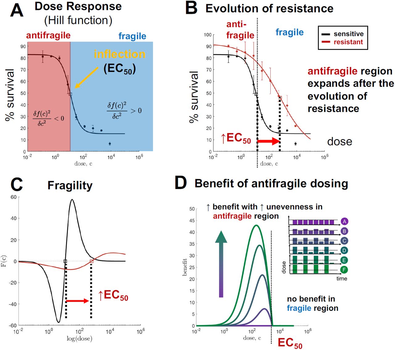
(A) Hill function best-fit (black) to HC122 treatment naive cells (circles with error bars). (B) Identical dose response assay, with evolved resistant cell line shown. (C) Fragility of naive and resistant lines, calculated from Hill function best fit. (D) Simulated percent benefit of uneven dosing schedules over continuous schedules.
Antifragility & resistance
These treatment-naive H3122 ALK-positive cell lines were exposed to a continuous 16 weeks of drug to create a drug-resistant population, termed “evolved-resistance” cell lines. Subsequently, resistant cell lines were assayed to the same treatment. After the evolution of resistance, the dose response curve shifts from left-to-right (figure 2B, red), resulting in an increased value of EC50. The dose-dependent fragility of both treatment-naive and resistant cells is shown in C.
Toxicity is a limiting factor when administering treatment in cancer patients. It may not be clinically feasible to continually increase the dose administered in the manner described in eqn. 2. In figure 2 we make the assumption that higher doses are exponentially less tolerable. Mathematically, this corresponds to a treatment cycle of (10c+σ, 10c−σ), or equivalently: plotting the curvature on a log-scale x-axis. In figure 2, the EC50 value represents the inflection point (on a log-scale) of the Hill function. Therefore, EC50 is the boundary line between the fragile region (where continuous therapy is optimal) and antifragile region (where uneven treatment is optimal).
Despite their ubiquity in cancer research, dose response assays are typically used to predict and measure differential response in first-order effects, (i.e. mean value of drug dose delivered) while second-order effects (i.e. convexity) are generally ignored. In clinical practice, doses are typically administered in the fragile region (where the dose is greater than the EC50), where continuous administration is optimal. However, figure 2 clearly shows that the antifragile regions expands after the evolution of resistance, indicating that a change in treatment schedule may be necessary. In D, the benefit to switching to an uneven schedule is shown. There is no benefit in the fragile region, but significant benefit in the low-dose antifragile region. Importantly, more unevenness is increasingly beneficial (shown by the color, with dosing schedules inset).
Fragility over time
When attempting control of a constantly evolving system, continuous monitoring and feedback is necessary to inform the timing of treatment decisions35. In figure 3, the rate of the loss of fragility and onset of antifragility is shown over time. H3122 cells under continuous exposure to Alectinib, are assayed every week for 10 weeks. Visually, treatment-naive cell lines (week 0) exhibit a convex, fragile curvature, which flattens out as cells are exposed to treatment. Although the dose response assay is only measured for three dose concentrations here, it is still possible to calculate a discrete measure of fragility.

(A) H3122 cells under continuous exposure to Alectinib, assayed every week for dose response at 3 concentrations (nM). (B) From A, the fragility can be directly calculated over time, with error shown for 3 biological replicates and 3 technical replicates. Note: due to an issue with data collection, week 5 is unfortunately omitted.
Antifragility & collateral sensitivity
One proposed solution to therapy resistance may lie in finding second-line therapies which have increased drug sensitivity to the resistant population of first-line treatment. This is known as collateral sensitivity, where the resistant state causes a secondary vulnerability to a subsequent treatment which was not previously present36. The antifragile-fragile framework can be extended to consider the optimal dose schedule for collaterally sensitive drugs. Here, we consider monotherapy of drug 1 administered until resistance evolves, then monotherapy of drug 2. As noted previously, cell lines were cultured in continuous exposure to a range of ten treatments (see table 1) to evolve resistance. Subsequently, evolved resistance cell lines were assayed to each of the ten treatments to examine potential collateral sensitivity34.
Figure 4A illustrates the magnitude and sign of fragility in response to Alectinib treatment for a treatment-naive (top), as well as the full range of evolved resistance cell lines. In each row, the antifragile region is colored red, and fragile colored blue. The black line shows the boundary line of treatment naive, with arrows indicating the shift after evolved resistance to ten other anti-cancer drugs. Here, all ten treatments show an expanded region of antifragility. In other words, any of these ten treatments would enlarge the antifragile response region for Alectinib.

(A) Magnitude and sign of dose response fragility. Vertical black line indicates the fragile-antifragile boundary for treatment-naive cells, and arrows indicate shift after evolved resistance to indicated treatment. (B) Collateral fragility: the shift for each pairwise sequence of treatments.
Likewise, every pairwise combination is shown in figure 4B, where a significant of sequential treatments are colored in red, indicating a potential improvement upon continuous therapy. The diagonal entries of this heatmap represent the shift of EC50 after evolved resistance to a single drug (as in the previous section). Seven of the ten drugs indicated an expansion of the antifragile (similar to figure 2).
Discussion
Over the past decades it has become increasingly clear that the benefit of a cancer therapeutic agent is determined not only by its molecular action but also by its schedule. However, because of the costs associated with clinical trials and the combinatorial size of the potential search space, optimal treatment strategies remain elusive. As a result, most therapies are administered in a fashion to maximize cell kill, meaning they are given as frequently as is logistically feasible (weekly for chemotherapies, daily for orally available targeted therapies) and at the maximum dose patients can safely tolerate. At the same time, translating into the clinic alternative schedules which have been shown to perform better in vitro, in vivo, and/or in silico has been challenging, and has failed on several occasions. For example, even though “bolus-dosing” of EGFR inhibitor for EGFR-Mutant NSCLC, in which daily low dose treatment is supplemented with a weekly high dose of therapy, was shown to better control therapy resistance than the standard-of-care continuous schedule in a mathematical model27, as well as in in vitro27 and in in vivo experiments28, it failed to do so in patients37.
One reason for this discrepancy is the fact that it is often difficult to understand why a given schedule is optimal. In this paper, we have shown how that the theory of antifragility, pioneered in financial risk management, provides a general tool to compare schedules in an intuitive yet formal fashion. In particular, we have demonstrated that the curvature of the dose response curve determines whether regimens should seek to maintain a constant treatment level, or should induce fluctuations between high and low periods of exposure. Importantly, this assessment can be made graphically and does not require specialist knowledge of complex optimization techniques. Moreover, it is easily generalizable as it can be applied to dose response curves obtained from any experimental or theoretical model system.
At the same time, antifragility is supported by a thorough mathematical foundation and we have illustrated how it may be quantified in order to allow formal comparison of different cell lines or therapeutic agents. We have shown that standard-of-care for TKI inhibitors in lung cancer (continuous administration of high doses) often are applied in so-called fragile regions, affirming the optimality of standard-of-care schedules. However, our results have also shown that this conclusion breaks down after 1) the evolution of resistance, and 2) the collateral sensitivity to a previous treatment. This suggests that treatment schedules are only “optimal” for limited periods of time, and will need to be adapted as the tumour changes in response to treatment.
Treatment adjustments to manage toxicity are commonplace in clinical practice, and work on so-called “adaptive therapy” has shown that adjustments based on tumour response are clinically feasible and beneficial25. This treatment paradigm attempts to capitalize on competition between tumor subclones21,38, by maintaining drug-sensitive cells in order to suppress resistant growth due the cost to resistance. There is recent evidence that cost of resistance may be environmentally driven, depending on availability of resources39, and may not be required for adaptive approaches to be effective40. We advocate for the further development of adaptive frameworks and believe that antifragility may provide useful metric to inform when and how the schedule should be modified. Adaptive approaches typically utilize drug holidays, attempting to re-sensitize tumors during drug relaxation periods. We propose to also monitor changes in fragility after drug is removed. For example, a study adaptively administering BRAF-MEK inhibitor treatment in BRAF-mutant melanoma found that drug holidays allowed for recovery of a transcriptional state associated with a low IC-50 value41. This re-sensitization of drug-sensitive phenotypes during drug holidays occurs only for one cell line, WM164, while a second line showed no re-sensitization (1205Lu). Visually, the dose response curves within this study are strikingly concave (antifragile) after evolved resistance, while only the WM164’s return to a convex, fragile state after drug holiday. Other adaptive approaches utilize dose modulation, adjusting the dose higher or lower dependent on tumor response. It is still an open question on how to design effective adaptive dose modulation42,43. The antifragility framework introduced here may provide a path forward to predicting whether “uneven” dose modulation may outperform continuous treatment.
While experimentally validating the link between the shape of the dose response curve and treatment scheduling will be the subject of future studies, evidence for our hypothesis can already be found in the literature. Aside from the just mentioned example in melanoma, the work by Chmielecki et al27 provides validation in NSCLC. The authors observe a concave (antifragile) dose response curve for partially or fully resistant tumour populations treated with erlotinib. As would be predicted by our hypothesis, subsequent experiments find that bolus dosing controls resistance for longer than continuous dosing27.
Clinicians have a “first-mover” advantage, enabling them to exploit cancer evolution by adopting more dynamic treatment protocols which integrate eco-evolutionary dynamics into clinical decision-making44. While it is difficult to calculate the patient-specific risk and timing of resistance, it is often more straightforward to predict the harm incurred if a line of treatment fails. As such, treatment regimens should be designed in such a way to minimize the impact of failure, and in fact ideally turn it into an advantage. The concept that cancer evolution may be clinically steered is gaining increasing traction, and work on collateral sensitivity has already shown that resistance to one agent may induce sensitive to another34. In addition, we have demonstrated that along with sensitivity also the optimal mode of treatment will change. Looking ahead we propose to extend the concept of antifragility to combination therapy and to investigate, for example, the effects of drug synergism and antagonism.
To conclude, we observe that environmental fluctuations have been shown to play a role not only in treatment response but in carcinogenesis in more general. One recent consensus statement introduced the concept of an “eco-index,” a measure of hazards (e.g. drug perfusion; infiltrating lymphocytes) and resources (e.g. concentration of ATP, glucose and other nutrients; degree of hypoxia; vascular density) within the tumor ecosystem45. For example, instability in microenvironmental resources may lead to selection of cancer cells with fast proliferation rates4,45. The role of environmental fluctuations on the evolutionary dynamics of competing phenotypes has been previously studied using mathematical models of spontaneous phenotypic variations in varied nutrient conditions46 and of the storage effect (buffered population growth and phenotype-specific environmental response)47. Likewise, the Warburg effect, high glycolytic metabolism even under normoxic conditions, may arise to meet energy demands posed by stochastic tumor environments48,49. As such, antifragility may provide a useful metric for viewing a tumor’s response to fluctuations in environmental conditions in more general.
Supplementary Information
To illustrate the efficacy of various fixed and random treatment dosing strategies, below we test therapeutic outcomes using a generalized model of tumor growth dynamics under treatment:
 where f (c), is the fractional kill rate induced by dose c, and g(n) is the untreated growth rate. Here we consider exponential growth, where g(n) = α. Note: fractional kill, f (c), is inversely related to cell survival: S(c) = 1 − f (c). This means that fragility is also inverted:
  . However, the naming convention is the same: antifragile dose response curves are those which benefit from uneven schedules. In the next section we will use this model to compare treatment schedules with identical cumulative dose.
Generalized tumor growth dynamics
Fixed dosing treatment schedules are simulated for two dose response functions: fragile (figure S1A; blue) and antifragile (figure S1A; red). Treatment is administered each day with varied dose unevenness (Δc) but identical mean dose  . For example, in figure S1B continuous therapy (zero dose unevenness) is shown in purple, with highly uneven schedule shown in green. Tumor size over time (subject to eqn. 4) is shown in figure S1C and D. Continuous therapy is ideal for fragile dose response (figure S1C) but inferior for antifragile dose response (figure S1D).
Next, we allow the dosing unevenness to be a random variable, drawn once per treatment cycle from a Gamma distribution (probability density function shown in figure S2A), defined as follows:

Note: the type of distribution here is not important; we choose Gamma to allow for skewed left and skewed right dosing schedules. Sample treatment schedules are shown in figure S2B, where low unevenness (approximating continuous therapy) schedules shown in purple and highly uneven in green.
The Gamma distribution is increasingly skewed right as the shape parameter, k, increases. Tumor size dynamics averaged over 10 treatment schedules for each value of k. Again, continuous therapy is ideal for fragile dose response (panel C) but inferior for antifragile dose response (panel D).
Acknowledgments
The authors gratefully acknowledge funding from the Physical Sciences Oncology Network (PSON) at the National Cancer Institute, U54CA193489, as well as the Cancer Systems Biology Consortium (CSBC) grant from the National Cancer Institute (grant no. U01CA23238). Authors are also supported by the Moffitt Cancer Center of Excellence for Evolutionary Therapy.


