

Abstract
The computation of tautomer rations of druglike molecules is enormously important in computer-aided drug discovery, as over a quarter of all approved drugs can populate multiple tautomeric species in solution. Unfortunately, accurate calculations of aqueous tautomer ratios—the degree to which these species must be penalized in order to correctly account for tautomers in modeling binding for computer-aided drug discovery—is surprisingly difficult. While quantum chemical approaches to computing aqueous tautomer ratios using continuum solvent models and rigid-rotor harmonic-oscillator thermochemistry are currently state of the art, these methods are still surprisingly inaccurate despite their enormous computational expense. Here, we show that a major source of this inaccuracy lies in the breakdown of the standard approach to accounting for quantum chemical thermochemistry using rigid rotor harmonic oscillator (RRHO) approximations, which are frustrated by the complex conformational landscape introduced by the migration of double bonds, creation of stereocenters, and introduction of multiple conformations separated by low energetic barriers induced by migration of a single proton. Using quantum machine learning (QML) methods that allow us to compute potential energies with quantum chemical accuracy at a fraction of the cost, we show how rigorous relative alchemical free energy calculations can be used to compute tautomer ratios in vacuum free from the limitations introduced by RRHO approximations. Furthermore, since the parameters of QML methods are tunable, we show how we can train these models to correct limitations in the underlying learned quantum chemical potential energy surface using free energies, enabling these methods to learn to generalize tautomer free energies across a broader range of predictions.
Introduction
The most common form of tautomerism, prototropic tautomerism describes the reversible structural isomerism involving the sequential processes of bond cleavage, skeletal bond migration and bond reformation in which a H+ is transferred [1]. According to the IUPAC Gold Book, tautomers can be defined by the general equilibrium shown below in which X, Y, and Z are any of C, N, O, or S:

Numerous chemical groups can show prototropic tautomerism. Common examples include keto-enol (shown in Figure 2), amide/imidic acid, lactam/lactim, and amine/imine tautomerism [2].
Tautomerism influences many aspects of chemistry and biology
Tautomerism adds a level of mutability to the static picture of chemical compounds. How chemists think about and represent molecules is still largely influenced by the work of Kekulé and Lewis from the dawn of the 20th century [3]. The widespread usage of notating and representing chemical structure as undirected graphs with atoms as nodes and bonds as edges (and bond types annotated as edge attributes like single, double and triple bond) dominates the field of chemistry (with the notable exception of quantum chemistry) [4]. Tautomers make a satisfying description of chemical identity difficult in such a framework, since they can instantaneously change their double bond pattern and connectivity table if confronted with simple changes in environment conditions or exist as multiple structures with different connection table and bond pattern at the same time [5].
The change in the chemical structure between different tautomeric forms of a molecule is accompanied by changes in physico-chemical properties. By virtue of the movement of a single proton and the rearrangement of double bonds, tautomerism can significantly alter a molecule’s polarity, hydrogen bonding pattern, its role in nucleophilic/electrophilic reactions, and a wide variety of physical properties such as partition coefficients, solubilities, and pKa [6, 7].
Tautomerism can also alter molecular recognition, making it an important consideration for supramolecular chemistry. To optimizing hydrogen bond patterns between a ligand and a binding site tautomerismn has to be considered. One of the most intriguing examples is the role that the tautomeric forms of the four building blocks of deoxynucleic acids played in the elucidation of biologically-relevant base pairings. The now well known Watson-Crick base pairing is only possible with guanine and cytosine in their amino (instead of imino) form and adenine and thymine in their lactam (instead of lactim) form. Watson and Crick struggled in their first attempts to get the tautomeric form of guanine right, delaying their work for a couple of weeks [2]. In the end, they concluded: “If it is assumed that the bases only occur in the most plausible tautomeric forms … only one specific pair of bases can bond together” [8]. The significance of this anecdote should not be underestimated. In a theoretical study of all synthetic, oral drugs approved and/or marketed since 1937, it has been found that 26% exist as an average of three tautomers [9]. While tautomerism remains an important phenomena in organic chemistry, it has not gained much appreciation in other scientific fields and there is little reason to doubt that such mistakes might repeat themselves in different settings [5].
The typical small energy difference between tautomers poses additional challenges for protein-ligand recognition. Local charged or polar groups in the protein binding pocket can shift the tautomer ratio and result in dominant tautomers in complex otherwise not present in solution [4]. For this reason the elucidation of the dominant tautomer in each environment is not enough — without the knowledge about the ratio (i.e. the free energy difference) between tautomeric forms in the corresponding phase a correct description of the experimental (i.e. macroscopic) binding affinity might not be possible. To illustrate this one might think about two extreme cases: one in which the tautomer relative solvation free energy is 10 kcal/mol and one in which it is 1.0 kcal/mol. It seems unlikely that the solvation free energy difference of 10 kcal/mol will be compensated by the protein binding event (therefore one could ignore the unlikely other tautomer form), but a tautomer solvation free energy difference of 1 kcal/mol could easily be compensated. Examples for this effect — changing tautomer ratios between environments — are numerous for vacuum and solvent phase. One example is the neutral 2-hydroxypyridine(2-HPY)/2-pyridone(2-PY) tautomer. The gas phase internal energy difference between the two tautomers is circa 0.7 kcal/mol in favor of the enol form (2-HPY), while in water an internal energy difference of 2.8 kcal/mol was reported in favour of 2-PY. In cyclohexane, both tautomer coexist in comparable concentration while the 2-PY is dominant in solid state and polar solvents [10].
The example above assumed two tautomeric forms — if there were multiple tautomeric forms, each with small free energy differences, using a single dominant tautomer in solvent and complex may still represent only a minor fraction of the true equilibrium tautomer distribution.
The study of tautomer ratios requires sophisticated experimental and computational approaches
The experimental study of tautomer ratios is highly challenging [11]. The small free energy difference and low reaction barrier between tautomers—as well as their short interconversion time—can make it nearly impossible to study specific tautomers in isolation. Also, tautomer ratios can be highly sensitive to pH, temperature, salt concentration, solvent and environment [9]. The majority of available quantitative tautomer data is obtained from NMR and UV-vis spectroscopy, in combination with chemometric methods [5]. Recently, efforts have been made to collect some of the experimental data and curate these in publicly available databases, specifically Wahl and Sander [12] and Dhaked et al. [13].
In the absence of a reliable, cheap, and fast experimental protocol to characterize tautomeric ratios for molecules, there is a need for computational methods to fill the gap. And — even if such a method exists — predicting tautomer ratios of molecules that are not yet synthesized motivates the development of theoretical models. Computational methods themselves have a great need for defined tautomer ratios. Most computational methods use data structures in which bond types and/or hydrogen positions have to be assigned a priori and remain static during the calculation, introducing significant errors if an incorrect dominant tautomer is chosen [14]. This is true for a wide variety of methods including molecular dynamics/Monte Carlo simulations (and free energy calculations based on them), quantum chemical calculations (heat and energy of formation, proton affinities, dipole moments, ionization potentials (e.g. Civcir [15])), virtual screening [16], QS/PAR, docking, many molecular descriptors, and pKa/logD/logP calculations [9].
In the last 20 years, a multitude of different studies (see Nagy [17, 18] for a good overview) have been conducted using a wide variety of methods ranging from empirical (e.g. Milletti et al. [16]), force field based [19] to quantum chemical calculations [20] to investigate tautomer ratios in solution (or, more generally, proton transfer).
The third round of the Statistical Assessment of the Modeling of Proteins and Ligands (SAMPL2) challenge included the blind prediction of tautomer ratios and provided an interesting comparison between different computational methods [21]. Most of the 20 submissions were using implicit solvent models and ab initio or DFT methods to evaluate the free energy differences [21]. Typically, such calculations use a thermodynamic cycle to assess the relative solvation free energy (as shown in Figure 1). The Gibbs free energy is calculated in vacuum and the transfer free energy added using a continuum solvation model to obtain the free energy in aqueous phase. The difference between the free energy in aqueous phase is the relative solvation free energy. However, as stated in Martin [22], “In summary, although quantum chemical calculations provide much insight into the relative energies of tautomers, there appears to be no consensus on the optimal method”. For the 20 tautomer pairs investigated in the SAMPL2 challenge (this includes 13 tautomer pairs for which tautomer ratios were provided beforehand) the three best performing methods reported an RMSE of 2.0 [23], 2.5 [24] and 2.9 kcal/mol [25]. While these results are impressive it also shows that there is clearly room for improvement. And, maybe even more importantly, the SAMPL2 challenge showed the need for investigating a wider variety of tautomer transitions to draw general conclusions about best practice/methods for tautomer predictions [21]. The excellent review of Nagy concluded that tautomer relative free energies are sensitive to “the applied level of theory, the basis set used both in geometry optimization and […] single point calculations, consideration of the thermal corrections […] and the way of calculating the relative solvation free energy” [17]. We’d like to add “quality of 3D coordinates” to these issues and discuss them in the following.

A typical quantum chemistry protocol calculates the free energy in aqueous phase  as the sum of the free energy in gas phase (
 ; calculated using the ideal gas RRHO approximation) and the standard state transfer free free energy (
 ; obtained using a continuum solvation model). The relative solvation free energy
  is then calculated as the difference between
  for two tautomers.
Standard approaches to quantum chemical calculations of tautomer ratios introduce significant errors
The relative solvation free energy  can be calculated from the standard-state Gibbs free energy in aqueous phase of the product and educt of the corresponding tautomer reaction. The free energy in aqueous phase of each tautomer
  is calculated as the sum of the gas-phase free energy
  and the standard state transfer free energy
  expressed as
 for a given conformation k and shown as a thermodynamic cycle in Figure 1.
The standard state gas phase free energy  of conformation k at temperature T is defined as
 with Ek as the electronic energy in the gas phase for a given conformation k, ϵZ PE,k the zero point energy (ZPE) correction,
  the thermal contribution to the Gibbs free energy for conformer k at temperature T and D the degeneracy of the ground electronic state in the standard state at 1 atm [26].
The standard-state Gibbs free energy is calculated using a quantum chemistry estimate for the electronic energy and, based on its potential energy surface, a statistical mechanics approximation to estimate its thermodynamic properties. While the accuracy of the electronic energy and the transfer free energy ΔGS is dependent on the chosen method and can introduce significant errors in the following we want to concentrate on the approximations made by the thermochemical correction to obtain the gas phase free energy: the rigid rotor harmonic oscillator approximation and the use of single or multiple minimum conformation/s to generate a discret partition function.
Rigid rotor harmonic oscillator can approximate the local configurational integral
A commonly used approach for the ZPE and thermal contributions is based on the ideal gas rigid rotor approximation (RRHO), assuming that the molecule is basically rigid and its internal motions comprise only vibrations of small amplitude where the potential energy surface can be approximated as harmonic around a local energy minimum. This assumption leads to an analytical approximation that describes the local configuration space around a single minimum based on the local curvature of the potential energy surface (Figure 2). The RRHO partition function QRRHO is assumed to be separable in the product of translational Qtrans, rotational Qrot, and vibrational Qvib terms. Using these approximations thermodynamic properties can be calculated using the molecule’s geometry, frequencies/normal modes, and electronic state [27].

The enol and keto form of a molecules (in the enol form: 1-(cyclohex-3-en-1-yl)ethen-1-ol) is shown and the main conformational degrees of freedom highlighted. The middle panel shows how the use of a local and harmonic approximation to the partition function can approximate the overall potential energy landscape, if all relevant minimum conformations are enumerated. The lower panel shows the probability density resulting from the harmonic approximations, with solid colored regions the difference between the true and approximated probability density resulting from anharmonicity and/or bonded terms that would better be modeled using a hindered/free rotor.
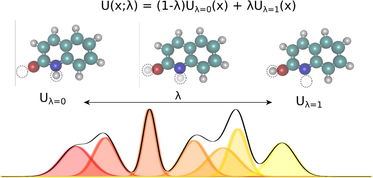
Linearly interpolating between two potential energy functions using the alchemical parameter λ enables the sampling of bridging distributions between the physical endstates representing the two tautomers. Here, non interacting dummy atoms—indicated by the empty circle at each endstate—are included to facilitate this transformation. In this work, we present the application of this concept to calculate relative free energies of tautomer pairs in vacuum.
Errors are introduced because the harmonic oscillator approximation assumes that, for each normal mode, the potential energy associated with the molecule’s distortion from the equilibrium geometry has a harmonic form. Especially low-frequency torsional modes would be more appropriately treated as hindered internal rotations at higher temperatures. This can lead to a significant underestimate of the configurational entropy, ignoring the contributions of multiple energy wells [28]. The correct treatment of such low-frequency modes in the analytical rotational entropy part of the RRHO partition function can add considerable computational cost, since the numerical solution requires the calculation of the full torsion potential (periodicity and barrier heights). Given that errors in the partition function are multiplicative and molecules may have several low-frequency torsional modes it is of interest to minimize their contribution to the final result [29].
Multiple local configurational integrals can be used to construct a discrete partition function
The free energy and all other standard thermodynamic properties of a system in a given thermodynamic ensemble are accessible through its partition function Q integrated over all possible conformations x [27]
 where u(x) denotes the reduced potential energy at coordinate set x. Given N local energy minima, the partition function can be approximated as a sum of N local integrals qk [30]. The local partition function qk restricted to energy well k can be written as
 with Q(k)RRHO as the RRHO partition function at the local minimum conformation kmin. The partition function Q can be approximated as a sum of contributions from the system’s predominant low-energy conformations.
The standard state free energy G° of a molecule can then be calculated from the molar thermodynamic functions (in detail described in e.g. [27]) for each of the minimum conformations separately and combined as follows
 to obtain a weighted free energy k [26, 31]. The free energy obtained in equation 5 mitigates the short-comings of the RRHO approach to model torsion with periodicity of 1 since — as long as the different minimas of the torsion are generated as conformations — these are included in the sum over all conformations.
Alchemical relative free energy calculations with machine learning potentials can compute true tautomer free energy differences, including all classical statistical mechanical effects
Limitations of the ideal gas RRHO approximation to the free energy and ZPE correction, challenges in enumeration of local minima, and the consistent treatment of internal/external rotational symmetry, as well as approximations in the continuum solvent model can lead to errors in the free energy that are difficult to detect and correct. The use of molecular dynamics simulations, explicit solvent molecules, and a rigorous classical treatment of nuclear motion to sample independent conformations from an equilibrium distribution can overcome the above mentioned challenges. To describe solvation free energies of tautomer pairs this would require computationally prohibitive QM/MM calculations in which the molecule of interest is treated quantum mechanically and the solute treated with molecular mechanics.
One of the most exciting developments in recent years has been the introduction of fast, efficient, accurate and transferable machine learning potentials (QML) (e.g. ANI [32], PhysNet [33], and SchNet [34]) to model organic molecules. QML potentials can be used to compute QM-based Hamiltonians and—given sufficient and appropriate training data—are able to reproduce electronic energies and forces without loss of accuracy but with orders of magnitude less computational cost than the QM methods they aim to reproduce. QML potentials have been successfully applied to molecular dynamics (MD) and Monte Carlo (MC) simulations [35]. Here, we present the application of a machine learning potential for the calculation of alchemical free energies for tautomer pairs in the gas phase.
We begin by investigating the accuracy of a current, state of the art approach to calculate tautomer ratios. We are using a popular DFT functional (B3LYP) and basis sets (aug-cc-pVTZ and 6-31G(d)) [36–40] for the calculation of the electronic energy and the continuum solvation model (SMD [41]) to model the transfer free energy. We are investigate its performance on a large set of diverse tautomer pairs spanning both different tautomer reactions, size and functional groups. We have selected a subset of 468 tautomer pairs from the publicly available Tautobase dataset [12] and performed quantum chemical geometry optimization, frequency calculation, single point energy, and thermochemistry calculations in gas and solvent phase using B3LYP/aug-cc-pVTZ and B3LYP/6-31G(d). This should significantly add to the canon of tautomer ratio studies.
Furthermore we are investigating the effect of a more rigorous statistical mechanics treatment of the gas phase free energies. To analyse this we calculate relative vacuum free energies between tautomer pairs  using (1) alchemical relative free energy calculations and (2) multiple minimum conformations in combination with the RRHO approximation (as used in the quantum chemistry approach). To enable a direct comparison between the two approaches we are using a QML potential for both approaches.
Since we are interested in relative solvation free energies we investigate the possibility to optimize the QML parmaters to include crucial solvent effects. The framework we have developed to perform alchemical relative free energy calculations for tautomer pairs enables us to obtain a relative free energy estimate that can be optimized with respect to the QML parameters. We are using a small training set of experimentally obtained relative solvation free energies  and importance sampling to obtain reweighted
  with the optimized parameters.
Here we report the first large scale investigation of tautomer ratios using quantum chemical calculations and machine learning potentials in combination with alchemical relative free energy calculations spanning a large chemical space and  values.
Standard quantum chemistry methods predict tautomer ratios with a RMSE of 3.1 kcal/mol for a large set of tautomer pairs
Calculating free energy differences between tautomer pairs in solution  is a challenging task since its success depends on a highly accurate estimate of both the intrinsic free energy difference between tautomer pairs as well as of their different contributions to the transfer free energy.
We calculated the relative solvation free energy  for 468 tautomer pairs (460 if the basis set 6-31G(d) was used) and compared the results with the experimentally obtained relative solvation free energy
  values in Fig 4. The full results for all methods are given in Figure S.I.1. Three quantum chemistry approaches were used to calculate these values:
B3LYP/aug-cc-pVTZ/B3LYP/aug-cc-pVTZ/SMD: Generating multiple conformations, optimizing with B3LYP/aug-cc-pVTZ in gas phase and solution phase (using the SMD continuum solvation model) and calculating
 as the difference of the free energy in aqueous phase for the individual tautomers. The free energy in aqueous phase is calculated as the sum of the free energy in gas phase (evaluated on the in gas phase optimized conformation) and the difference between the single point energy in gas phase (gas phase conformations) and solvent (solvent phase conformation) calculated on the B3LYP/aug-cc-pVTZ level of theory. The individual free energies in aqueous phase for conformation k are weighted to obtain the final . Conformations were filtered based on heavy atom and heteroatom hydrogens root means square displacement of atoms (RMSD) (described in detail in the Methods section). This approach will be abbreviated with B3LYP/aug-cc-pVTZ/B3LYP/aug-cc-pVTZ/SMD in the following. The RMSE between and for the dataset is 3.4 [3.0;3.7] kcal/mol (the quantities [X;Y] denote a 95% confidence interval).
B3LYP/aug-cc-pVTZ/B3LYP/6-31G(d)/SMD Generating multiple conformations, optimizing with B3LYP/aug-cc-pVTZ in gas phase and solution phase (using the SMD continuum solvation model) and calculating
as the difference between the free energy in aqueous phase for the individual tautomers. The free energy in aqueous phase is then calculated as the sum of free energy in gas phase (evaluated on the gas phase conformation) and the difference between the total energy in gas phase (evaluated on the gas phase conformation) and solvent phase (evaluated on the solvent phase conformation) on the B3LYP/6-31G(d) level of theory. The individual free energy in aqueous phase values for conformation k are then weighted to obtain the final . Conformations were filtered based on heavy atom and heteroatom hydrogens RMSD. The RMSE between and for the QM dataset is 3.1 [2.7;3.4] kcal/mol. This approach will be subsequently called B3LYP/aug-cc-pVTZ/B3LYP/6-31G(d)/SMDB3LYP/aug-cc-pVTZ/SMD Generating multiple conformations, optimizing with B3LYP/aug-cc-pVTZ in solution phase (using the SMD solvation model) and calculating relative solvation free energy
directly as the difference between the free energy in aqueous phase (and on the solution phase geometry). In this case, the free energy in aqueous phase is not obtained through a thermodynamic cycle, but the frequency calculation and thermochemistry calculations are performed with the continuum solvation model [42]. The individual free energy in aqueous phase for conformation k are averaged to obtain the final . Conformations were filtered based on heavy atom and heteroatom hydrogens RMSD. The RMSE between and is 3.3 [3.0;3.7] kcal/mol. This approach will be subsequently called B3LYP/aug-cc-pVTZ/SMD.


 with a RMSE of 3.1 kcal/mol.
The direction of the tautomer reaction is chosen so that the experimentally obtained relative solvation free energy  is always positive. Panel A shows
  as the difference between the sum of the gas phase free energy and transfer free energy for each tautomer plotted against the experimental relative solvation free energy
  . B3LYP/aug-cc-pVTZ is used for the gas phase geometry optimization and single point energy calculation and the ideal gas RRHO approximation for the thermal corrections. The transfer free energy is calculated on B3LYP/aug-cc-pVTZ optimized geometries (for solvation phase with SMD as the continuum solvation model) using B3LYP/6-31G(d) and SMD. Values in quadrant II indicate calculations that assign the wrong dominant tautomer species (different sign of
  and
and  ). Red dots indicate tautomer pairs with more than 10 kcal/mol absolute error between
  and
and  . These are separately shown in Table S.I.1. In Panel B, the top panel shows the kernel density estimate (KDE) and histogram of
  and
and  . The red line indicates zero free energy difference (equipopulated free energies). In the lower panel the KDE of the difference between
  and
and  is shown. MAE and RMSE are reported in units of kcal/mol. Quantities in brackets [X;Y] denote 95% confidence intervals. The Kullback-Leibler divergence (KL) was calculated using
  .
.
Tautomer pairs with absolute errors above 10 kcal/mol are shown.
The relative solution free energies  calculated with B3LYP/aug-cc-pVTZ/B3LYP/6-31G(d)/SMD are shown in Figure 4. The following discussion will concentrate on the results obtained with the best performing method (B3LYP/aug-cc-pVTZ/B3LYP/6-31G(d)/SMD). The results for all other methods are shown in the Supplementary Material Section.
The protocol used to obtain the results described above did not explicitly account for changes in internal rotors (only changes in the point group were accounted for). The results including changes in internal rotors are shown in Figure S.I.2 — the results are overall worse.
The best performing quantum chemistry method shows very good retrospective performance on the SAMPL2 tautomer set
Some of the tautomer pairs deposited in the Tautobase dataset were also part of the SAMPL2 challenge, specifically 6 out of 8 tautomer pairs of the obscure dataset (1A_1B, 2A_2B, 3A_3B, 4A_4B, 5A_5B, 6A_6B) and 8 out of 12 tautomer pairs of the explanatory dataset (7A_7B, 10B_10C, 10D_10C, 12D_12C, 14D_14C, 15A_15B, 15A_15C, 15B_15C) [21]. Comparing these molecules with the results of the SAMPL2 challenge— specifically with the results of the 4 participants with the best overall performance ([25], [43], [24], and [23])—helps assess the quality of the chosen approach. Since all four mentioned participants employed different methods, we will briefly describe the best performing methods of these publications for which results are shown in Table 1. The references to the methods used below are not cited explicitly, these can be found in the publications cited at the beginning of the following paragraphs.
All values are given in kcal/mol. The calculations for Klamt and Diedenhofen [25] were performed with MP2+vib-CT-BP-TZVP, for Ribeiro et al. [24] with M06-2X/MG3S/M06-2X/6-31G(d)/SM8AD, Kast et al. [23] with MP2/aug-cc-pVDZ/EC-RISM/PSE-3, and Soteras et al. [43] with MP2/CBS+[CCSD-MP2/6-31+G(d)](d)/IEF-MST/HF/6-31G). On this subset the presented approach was the second best method based on the total RMSE. Bracketed quantities [X,y] denote 95% confidence intervals.
Klamt and Diedenhofen [25] used BP86/TZVP DFT geometry optimization in vacuum and the COSMO solvation model. Free energy in solvation was calculated from COSMO-BP86/TZVP solvation energies and MP2/QZVPP gas-phase energies. Thermal corrections (including ZPE) were obtained using BP86/TZVP ZPE.
Ribeiro et al. [24] calculated the free energy in solution as the sum of the gas-phase free energy and the transfer free energy. The gas phase free energy was calculated using M06-2X/MG3S level of theory and the molecular geometries optimized with the same method. The corresponding transfer free energy were computed at the M06-2X/6-31G(d) level of theory with the M06-2X/MG3S gas-phase geometries using the SM8, SM8AD, and SMD continuum solvation models (Table 1 shows only the results with SM8AD, which performed best).
Kast et al. [23] optimized geometries in gas and solution phase (using the polarizable continuum solvation model PCM) using B3LYP/6-311++G(d,p). Energies were calculated with EC-RISM-MP2/aug-cc-pVDZ on the optimized geometries in the corresponding phase. The Lennard-Jones parameters of the general Amber force field (GAFF) were used.
Soteras et al. [43] used the IEF-MST solvation model parameterized for HF/6-31G(G) to obtain transfer free energy values. Gas phase free energy differences were obtained by MP2 basis set extrapolation using the aug-cc-pVTZ basis set at MP2/6-31+G(d) optimized geometries. Correlation effects were computed from the CCSD-MP2/6-31+G(d) energy difference [44].
The approach used in this work (B3LYP/aug-cc-pVTZ/B3LYP/6-31G(d)/SMD) performs well compared to the four approaches described above. For the total set of investigated tautomer pairs our approach has a RMSE of 2.2 [1.4,2.9] kcal/mol, making it the second best performing approach only outperformed by Kast et al. [23].
Interestingly to note is the difference in RMSE between the explanatory and blind dataset. Approaches that perform well on the blind data set are performing worse on the explanatory set and vice versa. This is to a lesser extent also true for our chosen approach—B3LYP/aug-cc-pVTZ/B3LYP/6-31G(d)/SMD performs worse for the explanatory tautomer set (RMSE of 2.5 [1.5,3.6] kcal/mol) than on the blind tautomer set (RMSE of 1.3 [0.7,1.7]), but in comparison with the other four approaches, it is consistently the second best approach.
Interesting to note are the three tautomer reactions 15A_15B, 15A_15C and 15B_15C from the explanatory data set. The absolute error for B3LYP/aug-cc-pVTZ/B3LYP/6-31G(d)/SMD are 5.24, 1.9, 2.8 kcal/mol. It appears that the used approach has difficulty to model 15B correctly, showing larger than average absolute errors whenever 15B is part of the tautomer reaction. Most likely the hydroxyl group in 15B is critically positioned and sensitive to partial solvent shielding by the phenyl ring, something that has been observed before [23].
The discrepancy between the different approaches (ours included) for the tautomer set show that it seems highly difficult to propose a single method for different tautomer pairs that performs consistently with a RMSE below 2.0 kcal/mol. This issue is made substantially worse by the many different ways methods can be used/combined and errors can be propagated/compensated during  calculations. While we believe that a RMSE of 3.1 kcal/mol is a good value for the chosen approach, especially when compared to the results of the SAMPL2 challenge, it is by far not a satisfying result. The accuracy, compared to the cost of the approach, is not justifiable and there is still a dire need for more accurate and cheaper methods to obtain relative solvation free energies for tautomer pairs.
The molecules with the highest absolute error between the calculated and experimental tautomer free energies in solution have common substructures
5 out of the 6 molecules with highest absolute error between experimental  and calculated relative solvation free energy
  (above 10 kcal/mol) have common scaffolds (values and molecules shown in the Supplementary Material Table S.I.1). molDWRow_1668, 1669, 1670 are all based on 5-iminopyrrolidin-2-one with either nitrogen, oxygen or sulfur on position 4 of the ring. molDWRow_1559 and molDWRow_853 both have methoxyethylpiperidine as a common substructure.
For the three analogues based on 5-iminopyrrolidin-2-one we want to note that the experimental values are estimated results based on a three-way tautomeric reaction [45]. While this might point to the unreliability of  , we can not draw any definitive conclusions here without repeating the underlying experiment.
Including multiple minimum conformations seems to have little effect on the accuracy of relative solvation free energies
The three approaches described above (B3LYP/aug-cc-pVTZ/B3LYP/6-31G(d)/SMD, B3LYP/aug-cc-pVTZ/B3LYP/aug-cc-pVTZ/SMD and B3LYP/aug-cc-pVTZ/SMD) consider multiple conformations to obtain the relative solvation free energy  . Obtaining the global minimum conformation is an important and well established task in quantum chemistry calculations. Figure 4 shows the free energies in gas phase difference between the highest and lowest energy minimum conformation for the molecules from the dataset generated with B3LYP/aug-cc-pVTZ/B3LYP/6-31G(d)/SMD. While the majority of the molecules have only a single minimum conformation, for molecules with multiple minima the difference in the free energy in gas phase emphasises the need and justifies the cost for a global minimum conformation search.
While the scientific community agrees on the importance of the global minimum for property calculations, the importance of considering multiple conformations for relative solvation free energy calculations has not been well established (e.g. [46]). The additional cost of frequency calculations (especially if an analytical Hessian is not available) on conformations other than the lowest energy one adds substantially to the overall cost of these calculations. If a single, minimum energy conformation is sufficient to obtain a good estimate for the free energy in gas phase a lot of computational time could be saved.
Figure 6 shows the results for the relative solvation free energies using the Boltzmann average over multiple minimum conformations plotted against the single global minimum conformation. The results indicate that using multiple minimum conformations do not significantly change the final result compared to using a single, global minimum structure. Only 12 tautomer pairs show an absolute error larger than 1 kcal/mol in the relative solvation free energy  between the two approaches. Much more relevant than including multiple conformations is locating the global minimum conformation (as clearly shown by Figure 5).

For each molecule, the number of minima Nconf is plotted against the difference between the corresponding highest and lowest obtained free energy in gas phase value. The majority of molecules have only a single minimum; molecules with multiple minima show substantial free energy differences between the minimum conformations highlighting the need for a global minimum search.

These results are based on the calculations with B3LYP/aug-cc-pVTZ/B3LYP/6-31G(d)/SMD. A shows the relative solvation free energy  obtained with multiple minima (m.m.) plotted against the global, single minimum (s.m.) relative solvation free energy
  . B shows the KDE and histogram of the difference between s.m.
  and m.m.
  . The comparison indicates that there is little benefit using multiple minimum structures over a single, global minimum considering the high costs of the former.
The quantum machine learning (QML) potential ANI1x can reproduce single-point energy differences between tautomers with high accuracy
The ANI family of machine learning potentials [32] were trained on a large dataset that spans conformational and configurational space and has shown astonishing accuracy and transferability in the prediction of molecular total energies. But ANI was not trained on tautomer species of molecules making an investigation in potential modelling errors of the neural net potential necessary.
To approach this question we calculated molecular total energies E with ANI1x and ω B97X/6-31G(d) on molecular conformations optimized with ω B97X/6-31G(d) for all tautomers in investigation. The difference between the total energies for a single tautomer (i.e.  and for tautomer pairs (i.e.
 ) are shown in Figure 7. Tautomer pairs were excluded if one of them failed to converge to a minimum conformation during the optimization resulting in the removal of 21 tautomer pairs.

The difference between ANI1x and omega B97x/6-31G(d) (the quantum chemical method ANI1x was trained on) for single point energy calculations and single point energy differences of tautomer pairs are shown. 21 molecules for which the energy minimization failed were excluded from the analysis.
Single point energy calculations were performed using ANI1x with a RMSE of 1.5 [1.3,1.6] kcal/mol and a MAE of 1.0 [0.9,1.1] kcal/mol. 11.6 % (81/696) of single point energy calculations had a difference greater than 2 kcal/mol to the reference QM level of theory.
The difference between two single point energy calculations with ANI1x and its reference QM level of theory for the tautomer pairs had a slightly higher RMSE of 1.8 [1.6,2.1] kcal/mol and a MAE of 1.3 [1.2,1.5] kcal/mol. 22.1% (77/348) of tautomer pairs had a difference greater than 2 kcal/mol to the reference QM level of theory. There seems to be a small quantity of error compensation—a MAE of 1.3 [1.2,1.5] kcal/mol is in accordance with the expected error propagation for uncorrelated measurements.
Alchemical relative free energy calculations with quantum machine learning potentials can rigorously capture classical statistical mechanical effects
Alchemical relative free energy calculations were performed for 354 tautomer pairs using 11 alchemical intermediate λ states in vacuum.
In the following, we will compare the relative free energies obtained using alchemical free energy calculations with the multiple minima, RRHO approximation using the same potential energy function (ANI1ccx) to assess potential errors in the thermochemistry corrections. We will also show how a small number of experimentally obtained relative solvation free energies between tautomer pairs can be used to incorporate crucial solvent effects and recover relative solvation free energies by importance weighting and QML parameter optimization from alchemical relative free energy calculations in vacuum.
RRHO ANI1ccx calculations show significant deviations from the alchemical relative free energy calculations
In the limit of infinite sampling alchemical relative free energy calculations approach the exact free energy difference. Alchemical relative free energy calculations can be used to quantify the error that a discrete partition function in the form of multiple minimum conformations and harmonic treatment of all bonded terms (including torsions and internal rotators) introduce—if the same electronic energy function is used for both calculations.
Since the simulation time of the individual lambda states for the alchemical relative free energy calculations were relatively short (200 ps) we ran multiple (5) experiments with randomly seeded starting conformations and velocities to detect systems for which the simulation time was clearly insufficient. In the following we will only use systems that had a standard deviation of less than 0.3 kcal/mol for the 5 independent relative free energy calculations. Applying this filter resulted in the removal of 65 tautomer pairs whose alchemical free energy calculations had not converged.
Results shown in Figure 8 for one of the 5 independent calculations indicate the average error that every relative free energy calculation based on the RRHO approximation introduces, regardless of the accuracy of the actual potential to model electronic energies. The mean absolute error of 0.9 kcal/mol should not be underestimated. Results shown in Table 1 would be significantly improved if an error of 0.9 kcal/mol could be compensated by running a protocol that samples the relevant conformational degrees of freedom to obtain an exact partition function.
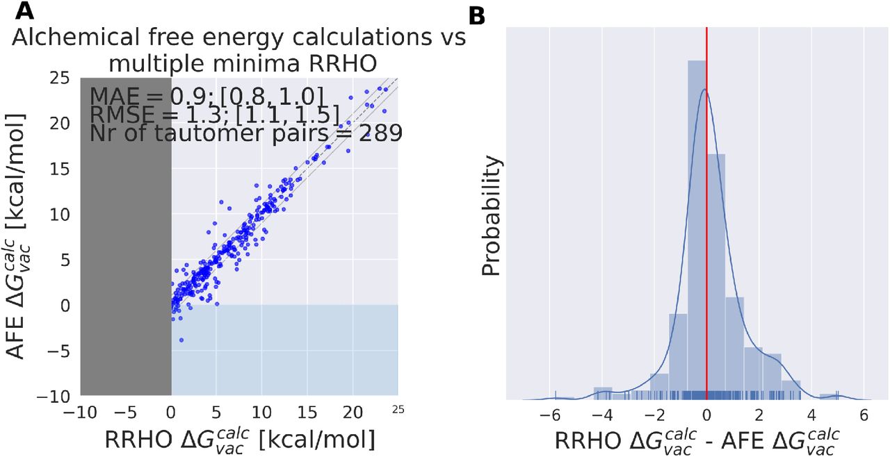
ANI1ccx is used for the calculation of relative gas phase free energies  using alchemical relative free energy calculations and single point energy calculations on multiple minimum conformations and thermochemistry corrections based on the RRHO approximation (RRHO). Results are shown for a single A shows a scatter plot between the two approaches and B the KDE and histogram of the difference between the two approaches. Error bars are shown in red on the alchemical relative free energy estimates, these were obtained from the MBAR estimate of the relative free energy (see Methods section).
For 12 (out of 289) tautomer pairs the multiple minima RRHO approximation introduces errors of more than 3 kcal/mol (molecules are shown in Figure 9). Most molecules shown have high conformational degrees of freedom and it seems unlikely that a naive conformational enumeration (like we used with a conformer generator) will detect all of them – this might contributed to the observed error. That is certainly true for molDWRow_113, 116, 565, 554, 403, 1674.
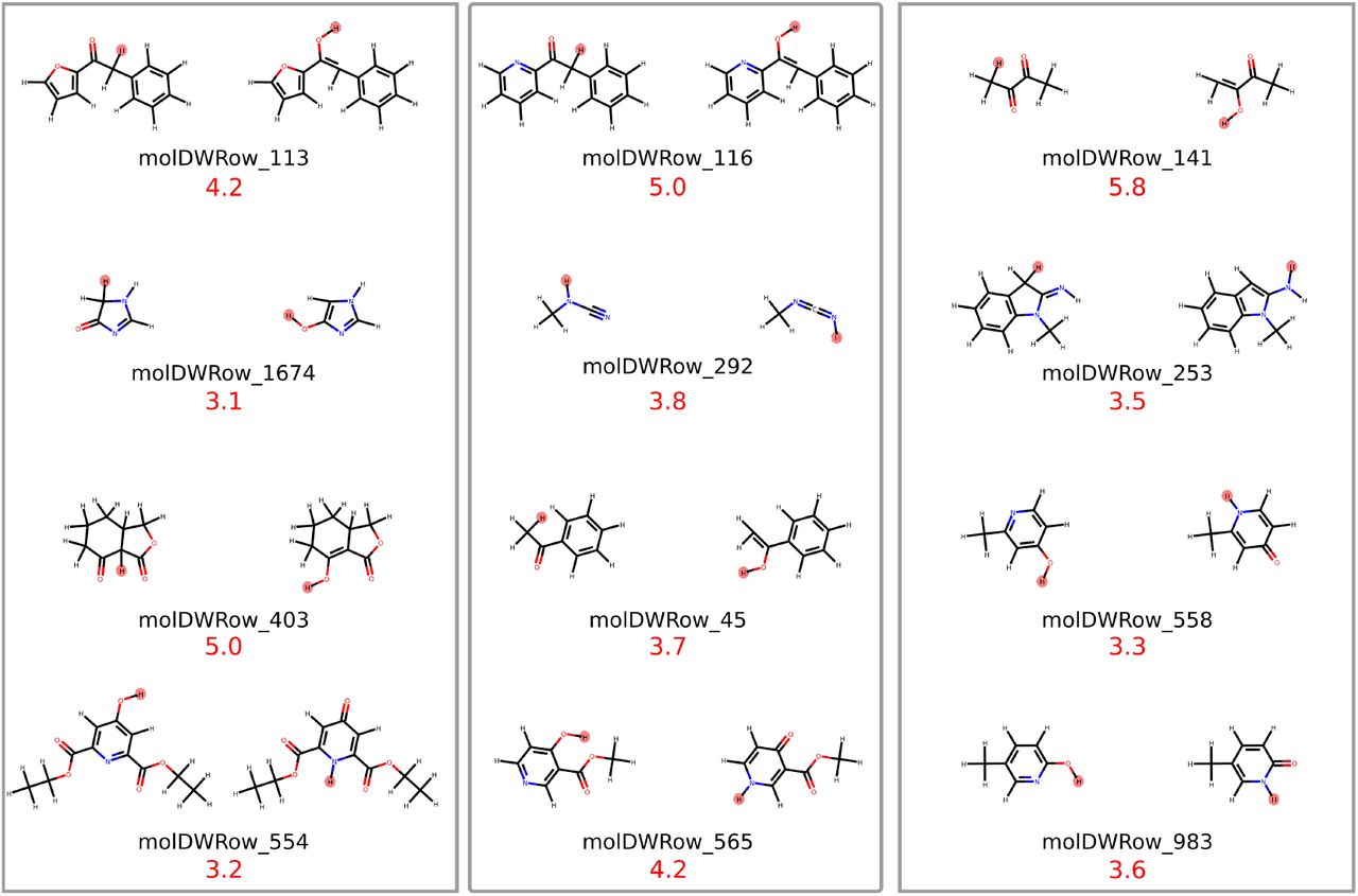
Absolute error is shown in red (value in kcal/mol) The hydrogen that changes position is highlighted in red.
QML potentials can be optimized to reproduce experimental relative solvation free energies
The aim of this section is to show that we can use optimized QML parameters to include solvent effects and perform importance weighting from vacuum simulations. The term relative gas phase free energy  is still used here, even though we aim to model relative solvation free energies
  .
.
Since the alchemical relative free energy calculations were performed in vacuum, a comparison with the experimental relative solvation free energies  showed a high RMSE of 6.4 [5.9,6.8] kcal/mol, as expected from the well-known impact of solvation effects on tautomer ratios [47].
Defining a loss function L as the mean squared error (MSE) between the relative calculated  and experimental
  free energies it is possible to minimize the loss with respect to the neural net parameters θ defining the ANI potential.
Using importance weighting, a new free energy estimate can be calculated with the optimized QML parameters (θ*) using the modified potential energy function without resampling the equilibrium distributions. Hereby, the accuracy of this estimate depends on the variability of the importance weights — the equilibrium distribution defined by the optimized QML parameters need to be fairly similar to work well (e.g. [48]). The used protocol is described in more details in the Methods section.
Figure 10 shows the obtained relative free energy estimates with the optimized QML parameters. The best performing QML parameters on the validation tautomer set were obtained after just two epochs of optimization (each including a single parameter optimization update per tautomer pair). Using validation-based early stopping the optimized QML parameters were used to calculate relative gas phase free energies  on an independent test set (71 tautomer pairs) show in Figure 10 B. The RMSE on the test set after optimization was decreased from 6.6 [5.4,7.8] kcal/mol to 3.1 [2.2,.8] kcal/mol, comparable to the performance of B3LYP/aug-cc-pVTZ/B3LYP/6-31G(d)/SMD.

 enables ANI1ccx to include crucial solvation effects and good estimates for relative solvation free energies can be obtained by importance weighting from vacuum simulations using the improved QML parameters.
A shows the training (green) and validation (purple) set performance (RMSE) as a function of epochs. Validation set performance was plotted with a bootstrapped 95% confidence interval. The best performing parameter set (evaluated on the validation set – indicated as the intersection between the two red dotted lines) was selected to compute the RMSE on the test set. Figure B shows the distribution of  for the tautomer test set (71 tautomer pairs) with the native ANI1ccx (θ) and the optimization parameter set (θ*). The Kullback-Leibler divergence (KL) was calculated using
  for the native ANI1ccx and
  for the optimized parameter set.
Figure 10 B shows the distribution of  . The Kullback-Leibler divergence (KL) was calculated using
  for the native ANI1ccx and
  for the optimized parameter set. The KL value for
  shows that overall the optimized parameter set is able to reproduce the distribution of the experimental solvation free energies closely.
These results highlight the incredible potential of differentiable energies w.r.t input parameters, making the powerful optimization of the parameters easily accessible.
Discussion & Conclusion
In this work we use a state of the art density functional theory protocol and continuum solvation model to calculate tautomer ratios for 460 tautomer pairs using three different approaches to model the solvent contributions. The best performing method uses B3LYP/aug-cc-pVTZ and the rigid rotor harmonic oscillator approximation for the gas phase free energies (calculated on B3LYP/aug-cc-pVTZ optimized geometries). The transfer free energy was calculated using B3LYP/6-31G(d)/SMD on geometries optimized in their respective phase (with B3LYP/aug-cc-pVTZ). This approach performs with a RMSE of 3.1 kcal/mol.
One possible source of error — independent of the method used to calculate the electronic energy and model the continuum electrostatics — are the thermochemical corrections used to obtain the standard state free energy. Typically, a analytical expression for the partition function is used that is based on the rigid rotor harmonic oscillator approximation. To obtain rigorous relative free energy estimates we implemented an alchemical relative free energy workflow using the ANI family of neural net (QML) potentials [32]. The method was implemented as a python package and is available here: https://github.com/choderalab/neutromeratio.
Using the same potential for the calculations based on the RRHO and performing alchemical relative free energy calculations we show that the RRHO approximation introduces a mean absolute error of circa 1 kcal/mol on the investigated tautomer data set. These errors can be attributed to anharmonicity in bonded terms, difficulties to enumerate all relevant minimum conformations, inconsistencies in combining shallow local energy wells as well as the inconsistent treatment of internal and external symmetry numbers.
The calculated alchemical free energies obtained using the methods implemented in the “‘Neutromeratio’” package can be optimized with respect to the parameters of the QML potential. Using a small set of experimentally obtained relative solvation free energies we were able to show that we can significantly improve the accuracy of the calculated free energies on an independent test set.
What should be noted here: the experimental values are relative solvation free energies, while we calculate relative gas phase free energies. The optimization routine on the experimental relative solvation free energies adds crucial solvent effects to the accurate description of the vacuum potential energy. The ANI family of QML and comparable QML potentials have opened the possibility to investigate tautomer ratios using relative free energy calculations without prohibitive expensive MM/QM schemes.
Obtaining accurate free energy differences between tautomer pairs in solvent remains an elusive task. The sublet changes and typically small difference in internal energies between tautomer pairs require an accurate description of electronic structures. Furthermore, solvent effects have a substantial effect on tautomer ratios; consequently, a proper descriptor of solvation is essential. The change in double bond pattern typically also induce a change in the conformational degrees of freedom and, related, in the conformation and rotational entropy. But — despite all of these challenges — we remain optimistic that further developments in fast and accurate neural net potentials will enable improved and more robust protocols to use relative free energy calculations to address these issues.
Code and data availability
• Input files, results and setup scripts: https://github.com/choderalab/neutromeratio
Author Contributions
Conceptualization: JDC, JF, and MW; Methodology: JDC, JF, and MW; Software: JF, and MW; Investigation: JF, and MW; Writing–Original Draft: JDC, JF, and MW; Writing–Review&Editing: JDC, JF, and MW; Funding Acquisition: JDC and MW; Resources: JDC and MW; Supervision: JDC and MW.
Funding
JF acknowledges support from NSF CHE-1738979 and the Sloan Kettering Institute. MW acknowledges support from a FWF Erwin Schrödinger Postdoctoral Fellowship J 4245-N28. JDC acknowledges support from NIH grant P30 CA008748, NIH grant R01 GM121505, NIH grant R01 GM132386, and the Sloan Kettering Institute.
Disclosures
JDC is a current member of the Scientific Advisory Board of OpenEye Scientific Software and a consultant to Foresite Laboratories. The Chodera laboratory receives or has received funding from multiple sources, including the National Institutes of Health, the National Science Foundation, the Parker Institute for Cancer Immunotherapy, Relay Therapeutics, Entasis Therapeutics, Silicon Therapeutics, EMD Serono (Merck KGaA), AstraZeneca, Vir Biotechnology, Bayer, XtalPi, Foresite Laboratories, the Molecular Sciences Software Institute, the Starr Cancer Consortium, the Open Force Field Consortium, Cycle for Survival, a Louis V. Gerstner Young Investigator Award, and the Sloan Kettering Institute. A complete funding history for the Chodera lab can be found at http://choderalab.org/funding
Detailed methods
Experimental data
The full dataset considered for this study was obtained from the DataWarrior File deposited in https://github.com/WahlOya/Tautobase (commit of Jul 23, 2019), described in detail in [12]. The dataset was sourced from the tautomer codex authored by P.W. Kenny and P.J. Taylor [45].
From the dataset a subset of tautomer pairs were considered that
were measured/calculated/estimated in aqueous solution
had a logK value between +/−10
had a numeric logK value
had no charged species
did not contain iodine
only a single hydrogen changed its position
476 of the 1680 deposited tautomer pairs had these properties. We added two tautomer pairs from the SAMPL2 challenge (Tautomer pair 2A_2B and 4A_4B) [21]. 478 unique tautomer pairs were considered for further analysis. Unique tautomer pairs means that the combination of the two tautomers has to be unique, not the individual molecule. In the following we will use an identifier containing the row number entry from the original DataWarrier file to identify molecules in the dataset, e.g. molDWRow_200 describing the tautomer pair at row number 200 in the original DataWarrior file.
The logK value was converted to free energy differences with  ln K. The free energy difference of the tautomer pairs obtained from the Tautobase are subsequently referenced as
  in contrast to the calculated values which are called ΔGcalc. While we call all values deposited in the Tautobase
  we want to point out that some of these values are estimated or calculated.
A closer inspection of some of the outliers identified incorrectly drawn structures in the database (Row entry: 1260,1261,1262,1263,1264,514,515,516,517,1587) – these 10 tautomer pairs were subsequently removed from all further analysis. Removing these 10 tautomer pairs resulted in 468 tautomer pairs. Additionally, 8 tautomer pairs (Row entry: 989, 581, 582, 617, 618, 83, 952, 988) were removed from calculations performed with the basis set 6-31G(d) dataset containing bromide since there are no parameters available.
For calculations that involved ANI we had to remove tautomer pairs from the dataset that contained elements not included in the ANI training set (only C,N,H,O) resulting in 369 tautomer pairs. Furthermore, all molecules with a stereobond that changed its position in both tautomers were removed (this affected 15 tautomer pairs: molDWRow_1637, molDWRow_510, molDWRow_513, molDWRow_515, molDWRow_517, molDWRow_518, molDWRow_787, molDWRow_788, molDWRow_789, molDWRow_810, molDWRow_811, molDWRow_812, molDWRow_865, molDWRow_866, molDWRow_867).
The subset of the Tautobase used for the QM calculations can be obtained here as list of SMILES (468 tautomer pairs): https://github.com/choderalab/neutromeratio/blob/master/data/b3lyp_tautobase_subset.txt. The subset of the Tautobase used for the QML calculations can be found here as list of SMILES (354 tautomer pairs): https://github.com/choderalab/neutromeratio/blob/master/data/ani_tautobase_subset.txt. The distribution of the experimental solvation free energies for both datasets are shown in 11.
Generating molecular conformations
The input tautomer pairs were specified as SMILES strings. 3D conformations were generated with the chemoinformatics toolkit RDKit (version 2019.09.2) which uses the distance geometry approach to generate conformations while enforcing chirality/stereochemistry [49, 50] For each molecule 20 conformations were initially generated. The number of conformations was reduced to 10 if the average root mean square deviation (RMSD) of atoms of the 20 conformations was below 0.5 Angstrom, and further reduced to 5 conformations if below 0.2 Angstrom.
RMSD calculations and filtering of conformations
For each molecule, pairwise RMSD between conformations were calculated using RDKit. Starting with a random conformation, if the RMSD to any other conformation of the molecule was below 0.1 the conformation is discarded, otherwise added to the list of unique conformations. The RMSD was calculated between heavy atoms and the hydrogen of selected chemical moieties including primary alcohols, imines, primary/secondary amines, cyanamides and thiols.
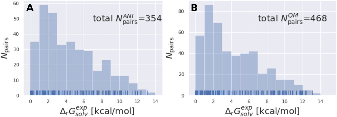
The tautomer dataset shows a wide variety of solvation free energies  . A shows the ANI-Tautobase subset that was used for the QML calculations and B shows the QM-Tautobase subset used for the QM calculations. The full dataset considered for this study was obtained from the DataWorrier File deposited at https://github.com/WahlOya/Tautobase (commit of Jul 23, 2019), described in detail in [12]. The selection criteria for both datasets are described in detail in Detailed methods section.
Quantum mechanical calculations
Orca and continuum solvation models for tautomer free energy calculations
Quantum mechanical calculations were performed using the quantum chemical software orca 4.0.1.2 [51].
Geometric optimization was performed with the standard options of orca, redundant internal coordinates and the BFGS optimizer using B3LYP/aug-cc-pVTZ [36–38] in vacuum and with a continuum solvation model. The universal solvation model based on solute electron density (SMD) was used as continuum solvation model [41].
Frequency calculations were performed with the numerical Hessian computed using the central differences approach. If a conformation had negative frequencies (imaginary modes) after the geometry optimization it was excluded from further analysis. Single point calculations were performed on the optimized geometries using B3LYP/aug-cc-pVTZ and B3LYP/6-31G(d) [39, 40] in vacuum and in the continuum solvation model. A damping dispersion correction was applied (orca keyword D3BJ) [52].
Thermal corrections were computed at standard state (298.15 K and 1 atm pressure) using the ideal gas molecular partition function and the rigid-rotor harmonic oscillator (RRHO) approximation. Since there is a volume change in the standard state from the gas phase (1 atm) to the solvent phase we indicate each phase either with ‘*‘ (gas phase standard state) or with ‘o’ (solution standard state). Low-lying vibrational frequencies (below 15 cm-1) were treated by a free-rotor approximation [53] – this method is also sometimes called rigid-rotor quasi harmonic oscillator.
The rotational symmetry number was obtained from the point group of the tautomer using the point group module of Jmol and visual inspection [54].
The Gibbs free energy in gas phase  was then obtained by adding thermal corrections
  (and ϵZ PE,k) to the electronic energy Ek for a given coordinate set (k).

The degeneracy D was estimated by calculating the graph automorphism of the molecule. The implementation of the VF2 algorithm for graph isomorphism of networkx (https://networkx.github.io/documentation/stable/citing.html) was used. Nodes were defined to match if element and hybridization matched, edges were identical if bond order matched.
SMD is used to model the molecules in aqueous environment. The standard-state transfer free energy is then defined as
 with ΔG∗→° as standard-state adjustments (specifically, the correction of changing the volume from the gas phase to the solute phase with a constant value of 1.89 kcal/mol), ΔGENP describes the electronic (E), nuclear (N) and polarization (P) components of the free energy and ΔCDS free energy changes associated with solvent cavitation (C), changes in dispersion (D) and changes in local solvent structure (S) [41]. The relative solvation free energy was computed as the difference in the free energies of both tautomer species.
Another possible way to calculate a relative solvation is to carry out the electronic structure calculation in the continuum solvation reaction field and using the ideal gas molecular partition function in combination with the RRHO approximation to obtain directly a free energy in aqueous phase. The free energy in aqueous phase is calculated using
 where ψsol is the polarized wave function in solution, Hg the gas phase Hamiltonian, and V the potential energy operator associated with the reaction field. The bracket term describes the electronic energy, while GNES is associated with non-electrostatic contributions (dispersion-repulsion and solvent structural terms) to the solvation energy and GT,K are the thermal correction calculated directly in the continuum solvation model [55].
We calculated the relative solvation free energy  for 468 tautomer pairs using three approaches. Generating multiple conformations, optimizing with B3LYP/aug-cc-pVTZ in gas phase and solution phase (using the SMD solvation model) and calculating the free energy in aqueous phase
  as the sum of the free energy in gas phase (evaluated on the gas phase conformation) and the transfer free energy using the B3LYP/aug-cc-pVTZ level of theory. The individual Gsolv,k for conformation k are then Boltzmann averaged to obtain the final Gsolv. The difference between the free energy in aqueous phase Gsolv for both tautomers is then the relative solvation free energy
Generating multiple conformations, optimizing with B3LYP/aug-cc-pVTZ in gas phase and solution phase (using the SMD solvation model) and calculating the free energy in aqueous phase  as the sum of the free energy in gas phase (evaluated on the gas phase conformation) using B3LYP/aug-cc-pVTZ and the transfer free energy using the B3LYP/6-31G level of theory. The individual Gsolv,k for conformation k are then Boltzmann averaged to obtain the final Gsolv. The difference between the free energy in aqueous phase Gsolv for both tautomers is then the relative solvation free energy
  .
.
Generating multiple conformations, optimizing with B3LYP/aug-cc-pVTZ in solvent phase (using the SMD solvation model) and calculating  directly as the difference between the IG-RRHO free energy calculated in solution (and on the solution phase geometry). The individual free energy in aqueous phase Gsolv,k for conformation k are Boltzmann averaged to obtain the final Gsolv.
Single point energy calculations with psi4
The electronic structure calculation was performed using the ωB97X density functional and the 6-31G(d) basis set with the quantum chemical program psi4 [56]. Geometric optimization was performed using redundant internal coordinates and BFGS Hessian updates. Using the optimized geometry electronic structure calculations were performed with machine learning potential ANI1x [32] as implemented in torchANI.
ASE thermochemistry corrections
For each molecule 100 conformations were generated. ANI1ccx was used to calculate the electronic energy. The conformations were minimized using the BFGS optimizer as implemented in scipy. Frequency and thermochemistry calculations were performed using the optimized geometry. Thermal corrections were calculated for 298 K and 1 atm using the IG-RRHO approximation as implemented in the atomic simulation environment (ase) [57]. The relative free energy in gas phase ΔGvac was then calculated as the difference between  of the tautomer pair.
Relative alchemical free energy calculations
Relative alchemical free energies were calculated using a single, hybrid topology approach for gas phase and solvation phase. The topology of each tautomer pair only differed in the position of a single hydrogen (bonds and bonded types were not specified). The hybrid topology (the superset of the two topologies) differed therefore by one hydrogen from each of the physical endstates.
As default, the coordinates of the hybrid topology were generated by using the coordinates of tautomer 1 (as defined in the initial tautomer database). If a tautomer isomerismn created or removed a cis/trans stereobond, the initial coordinates were taken from the topology with the stereobond present (therefore sometimes changing the direction of the tautomer reaction).
The coordinates of the added, non-interacting hydrogen were obtained by randomly sampling 100 hydrogen positions around its new bonded heavy atom and subsequently using the lowest energy position. The physical endstates (representing the two tautomer states, each with an additional non-interacting (dummy) hydrogen) were connected via 11 intermediate (lambda) states.
Energy and forces were calculated using ANI1ccx and ANI1x as implemented in torchani https://github.com/aiqm/torchani). The energy as well as the resulting force was linearly scaled along the alchemical path as a function of lambda with

Before each simulation, initial coordinates were minimized using BFGS optimizer as implemented in scipy. Coordinates were sampled using Langevin dynamics at 300 K with a collision rate of 10 ps−1 and a 0.5 fs time step using the BAOAB integrator [58]. Initial velocities were obtained from a Maxwell-Boltzmann distribution at the simulation temperature.
200 ps simuation time was used to obtain smaples from each lambda state Simulation The gas phase simulations were repeated 5 times with randomly seeded initial velocities (and coordinates).
All bonds involving hydrogens were restrained throughout the simulation at each lambda states using a flat bottom potential well with harmonic walls. The restraint was defined as
 with H as the Heaviside step function,
  as the difference between the reference bond length
  and the current bond length ri,j and rfb as half of the well radius. For all heavy atom pairs
  was set to 1.3 Angstrom and rfb to 0.3 Angstrom. For C-H/O-H/N-H bond pairs
  was set to 1.09/0.96/1.01 Angstrom and rfb to 0.4 Angstrom.
Relative alchemical gas phase free energies  were calculated using MBAR as implemented in the pymbar package [59]. To remove correlated snapshots from the MBAR analysis the time series functions of pymbar were used to detect the equilibrated region of the trajectory. 300 uncorrelated snapshots were considered for the MBAR analysis for each lambda state.
Neural net parameter optimization based on experimental relative solvation free energies
The tautomer data set was split into a test set (71 tautomer pairs), validation set (57 tautomer pairs) and training set (226 tautomer pairs). Gradient updates were performed on the training set, the best model was validated based on the RMSE on the validation set and used to evaluate the model performance on the test set.
Neural net parameters were optimized using a routine modified from the TorchANI tutorial1. To limit the capacity to overfit, only the weights and biases of the final layer of each of the 8 pretrained ANI-1ccx models were optimized for each of the atom nets (one net per element). As in the TorchANI tutorial, the weight matrices were updated using the Adam optimizer with decoupled weight decay, and the bias vectors were updated using Stochastic Gradient Descent (SGD). The weight decay rate was set to 10−6.
The model was trained by minimizing the MSE loss between calculated and experimental relative free energies. The per molecule pair (m) loss function l is defined as
 with
with  as the experimental and
  as the calculated relative free energy value for molecule m at parameters θ.
  is a function of the individual energies per lambda state, which are a function of the input parameters θ and the coordinate set. The overall loss is then

The perturbed relative free energy  required for computing l(m; θ) is calculated by importance sampling, or “reweighting” the original MBAR estimate from the original pre-trained parameters θ* to the current parameters θ. To compute this estimate efficiently at arbitrary θ, we first collect configuration samples at a reference value θ* (corresponding to the original parameters of the pretrained ANI-1ccx model) for each intermediate value λ. For each configuration sample x, we compute the reduced potential u(x,λ;θ*), to form the N × M matrix of inputs to MBAR. (Where N is the total number of snapshots, M is number of λ windows.) MBAR equations are solved to yield a vector of reduced free energies
  , where m indexes the intermediate λ values. The relative free energy prediction implied by the model parameters θ* is then
  .
.
To compute relative free energies at a new value of the parameters θ, we need to compute u(x, λ = 1; θ) and u(x, λ = 0; θ) for all configurations x. The optimization routine evaluates the gradient of the loss function L w.r.t. θ by automatic differentiation and updates the parameters.
300 uncorrelated snapshots per λ state were used for the MBAR estimate and importance sampling for the vacuum simulations.
Supplementary Information

Each of the three blocks show the QM calculations done with different level of theory indicated by the title in the plots in column A. In each block the top penal shows the results obtained with multiple minimum conformations, the bottom penal shows the results obtain with a single conformation. Column D shows the difference between the multiple minimum and single minimum approach and E show the the number of minimum conformations against the difference between the lowest and highest energy for each tautomer. These results were obtained without the additional structure symmetry correction.

Each of the three blocks show the QM calculations done with different level of theory indicated by the title in the plots in column A. In each block the top penal shows the results obtained with multiple minimum conformations, the bottom penal shows the results obtain with a single conformation. Column D shows the difference between the multiple minimum and single minimum approach and E show the the number of minimum conformations against the difference between the lowest and highest energy for each tautomer. These results were obtained with structure symmetry correction.
Acknowledgments
MW, JF and JDC are grateful for discussions from the Tautomer Consortium, specifically Paul Czodrowski, Brian Radak, Woody Sherman, David Mobley, Christopher Bayly and Stefan Kast as well as input from Adrian Roitberg and Olexandr Isayev. This work was only possible through the time and effort Thomas Sander and Oya Wahl invested in curating the open tautomer database (Tautobase). Further, MW is grateful for the support of Thierry Langer, who donated significant computational resources to perform much of the calculations/simulations and Oliver Wieder, for helpful discussions.
Footnotes
Results section notation clarified, updated title of Figure 4 and updated error bars on Figure 8. Notation of free energy terms clarified.
↵1 https://aiqm.github.io/torchani/examples/nnp_training.html
References
- [1].↵
- [2].↵
- [3].↵
- [4].↵
- [5].↵
- [6].↵
- [7].↵
- [8].↵
- [9].↵
- [10].↵
- [11].↵
- [12].↵
- [13].↵
- [14].↵
- [15].↵
- [16].↵
- [17].↵
- [18].↵
- [19].↵
- [20].↵
- [21].↵
- [22].↵
- [23].↵
- [24].↵
- [25].↵
- [26].↵
- [27].↵
- [28].↵
- [29].↵
- [30].↵
- [31].↵
- [32].↵
- [33].↵
- [34].↵
- [35].↵
- [36].↵
- [37].
- [38].↵
- [39].↵
- [40].↵
- [41].↵
- [42].↵
- [43].↵
- [44].↵
- [45].↵
- [46].↵
- [47].↵
- [48].↵
- [49].↵
- [50].↵
- [51].↵
- [52].↵
- [53].↵
- [54].↵
- [55].↵
- [56].↵
- [57].↵
- [58].↵
- [59].↵


