

1 Abstract
Collective dynamics in multicellular systems such as biological organs and tissues plays a key role in biological development, regeneration, and pathological conditions. Collective dynamics - understood as population behaviour arising from the interplay of the constituting discrete cells - can be studied with mathematical models. Off- and on-lattice agent-based models allow to analyse the link between individual cell and collective behaviour. Notably, in on-lattice agent-based models known as cellular automata, collective behaviour can not only be analysed through computer simulations, but predicted with mathematical methods. However, classical cellular automaton models fail to replicate key aspects of collective migration, which is a central instance of collective behaviour in multicellular systems.
To overcome drawbacks of classical on-lattice models, we introduce a novel on-lattice, agent-based modelling class for collective cell migration, which we call biological lattice-gas cellular automaton (BIO-LGCA). The BIO-LGCA is characterised by synchronous time updates, and the explicit consideration of individual cell velocities. While rules in classical cellular automata are typically chosen ad hoc, we demonstrate that rules for cell-cell and cell-environment inter-actions in the BIO-LGCA can also be derived from experimental single cell migration data or biophysical laws for individual cell migration. Furthermore, we present elementary BIO-LGCA models of fundamental cell interactions, which may be combined in a modular fashion to model complex multicellular phenomena. Finally, we present a mathematical mean-field analysis of a BIO-LGCA model that allows to predict collective patterns for a particular cell-cell interaction. A Python package which implements various interaction rules and visualisations of BIO-LGCA model simulations we have developed is available at https://github.com/sisyga/BIO-LGCA.
Author summary Pathophysiological tissue dynamics, such as cancer tissue invasion, and structure formation during embryonic development, emerge from individual inter-cellular interactions. In order to study the impact of single cell dynamics and cell-cell interactions on tissue behaviour, one needs to develop space-time-dependent agent-based models (ABMs), which consider the behaviour of individual cells. Typically, in agent-based models there is a payoff between biological realism and computational cost of corresponding model simulations. Continuous time ABMs are typically more realistic but computationally expensive, while rule- and lattice-based ABMs are regarded as phenomenological but computationally efficient and amenable to mathematical analysis. Here, we present the rule- and lattice-based BIO-LGCA modelling class which allows for (i) rigorous derivation of rules from biophysical laws and/or experimental data, (ii) mathematical analysis of the resulting dynamics, and (iii) computational efficiency.
3 Introduction
Systems biology and mathematical modelling is rapidly expanding its scope from the study of single cells to the analysis of collective behaviour in multicellular tissue- and organ-scale systems. In such systems, individual cells may interact with their environment (hapto- and chemotaxis, contact guidance, etc.) or with other cells (cell-cell adhesion, contact inhibiton of locomotion, etc.) and produce collective patterns exceeding the cells’ interaction range. To study collective behaviour in such systems theoretically and/or computationally, a mathematical model must be decided upon as a first step. Continuous models describe the average behaviour of the cellular population. Their lack of resolution at the individual level makes them inappropriate to study the role of individuals in collective behaviour. Agent-based models, on the other hand, are particularly suited to the study of collective behaviour in multicellular systems, as they resolve individual cell dynamics, and thus allow for the analysis of large-scale tissue effects of individual cell behaviour.
In the context of multicellular tissue dynamics, various agent-based models have been developed to analyse tissue dynamics as a collective phenomenon emerging from the interplay of individual biological cells. In these models, cells are regarded as separate, individual units, contrary to continuum methods, which neglect the discrete individual cell nature, and where tissue dynamics is derived from conservation and constitutive laws, drawing parallels to physical systems. Since agent-based models represent individual biological cells, distinct cell phenotypes can be taken into account, which may be fundamental for the organisation at the tissue level. For example, it has been shown that cell-to-cell variability plays a key role in tumour progression and resistance to treatment [1]. Moreover, with the advance of high performance computing, agent-based models can be used to analyse in vitro systems at a 1:1 basis even for large cell population sizes.
Agent-based models can be classified into on-lattice and off-lattice or “lattice-free” models depending on whether cell movement is restricted to an underlying lattice (see [2] for references). While lattice-free models are typically very detailed in their biophysical description, they are often too complex for mathematical analysis, while lattice models are normally very abstract and phenomenological, thus facilitating their analysis, but making biological data integration at the model definition level challenging.
In lattice models, either (i) a lattice site may be occupied by many biological cells (e.g., [3]), (ii) a site may be occupied by at most one single biological cell (e.g., [4]), or (iii) several neighbouring lattice sites may represent a single biological cell (e.g., [5]). In probabilistic lattice models, the interacting particle system (IPS) is an important example, proliferation, death, and migration of biological cells are modeled as stochastic processes. Model types (i) and (ii) can mimick volume exclusion effects, (iii) can qualitatively capture cell deformation and compression, while each of the three approaches can describe the effects of mechanical forces of one cell on its neighbour, or on a group of neighbouring cells to some extent.
Lattice models are equivalent to cellular automata, which have been introduced by J. v. Neumann and S. Ulam in the 1950s as models for individual (self-)reproduction [6]. A cellular automaton consists of a regular spatial lattice in which each lattice node can assume a discrete, typically finite number of states. The next state of a node solely depends on the states in neighbouring sites and a deterministic or stochastic transition function. Cellular automata provide simple models of self-organising systems in which collective behaviour emerges from an ensemble of many interacting “simple” components - being it molecules, cells or organisms [7, 8, 9, 10].
However, when modeling collective migration phenomena, classic CA and IPS models have major drawbacks which are due to the strict volume exclusion and asynchronous update in such models. Most importantly, they fail to produce collective movement at unit density, since this density implies a “jammed state” due to volume exclusion. These are for example the “traffic jams” in [11]. However, a fluidized state at unit density is important in epithelia. Furthermore, asynchronous update may lead to oscillating density spikes. For example in an IPS model for persistent motion in a crowded environment, cells at the invasion front detach and leave gaps behind that are subsequently filled by following cells [12]. This is an artefact of models with asynchronous update as in reality invasion can happen while cells stay connected all the time. Moreover, classic CA models consider only cell position and not explicitly cell momentum, complicating the modeling of collective cell migration mediated primarily through changes in momentum, rather than density.
The lattice-gas cellular automaton (BIO-LGCA) introduced here, on the other hand, is a cellular automaton in which lattice sites are updated synchronously, and which explicitly considers individual cell velocities. These features make the BIO-LGCA appropriate for modeling collective migration phenomena where cell interactions result in directional changes of velocity, and where high cell densities do not hamper movement. Table 1 presents an overview of on-lattice cell-based models.
Comparison of on-lattice cell-based models with respect to time representation, computational efficiency, migration modelling capacity, and availability of analytic methods. CA: cellular automaton, BIO-LGCA: biological lattice-gas cellular automaton, IPS: interacting particle system, CPM: cellular Potts model; for details see also [2].
The structure of the paper is as follows: we first formally define the BIO-LGCA model class. Then, we construct biophysical BIO-LGCA rules from microscopic Langevin models for selected cases of single and collective cell migration. Subsequently, we demonstrate how to generate data-driven BIO-LGCA rules from experimental single cell migration data (Fig. 1). Furthermore, we show that, in specific cases, the biophysical and the data-driven approaches converge to the same functional form. For this case, we present several simple, but biologically relevant model examples. We end with a critical discussion of the BIO-LGCA modelling framework.

BIO-LGCA modelling: The key question is to extract the interaction rules underlying a particular collective behaviour in a population of cells. Appropriate BIO-LGCA interaction rules can be chosen ad hoc, extracted from experimental single cell migration data, or derived from biophysical equations for single cell migration.
4 Definition
A BIO-LGCA is defined by a discrete spatial lattice  , a discrete state space
  , a neighbourhood
  and local rule-based dynamics.
4.1 Lattice
The regular lattice  consists of nodes
  . Every node has b nearest-neighbours, where b depends on the lattice geometry. Each lattice node
  is connected to its nearest neighbours by unit vectors ci, i = 1, …, b, called velocity channels. In addition, a variable number a ∈ ℕ0 of rest channels (zero-velocity channels) cj = 0, b < j ≤ a + b, is allowed (Fig. 2). The parameter K = a + b defines the maximum node capacity.

Lattice and neighbourhood in the BIO-LGCA: example of square lattice (left). The node state is represented by the occupation of velocity channels (right); in the example, there are four velocity channels c1, c2, c3, c4, corresponding to the square geometry of the lattice, and one “rest channel” c0. Filled dots denote the presence of a cell in the respective velocity channel; right: von Neumann neighbourhood (green) of the red node.
4.2 Neighbourhood
The set  , the neighbourhood template, defines the nodes which determine the dynamics of the node
  . Throughout this work, the neighbourhood will be assumed to be a von Neumann neighbourhood (Fig. 2), defined as
  , but other neighbourhood choices are possible. In general,
  , specifies the set of lattice nodes which determine the dynamics of the state at node
  . 1
. 1
4.3 State space
The state space in LGCA is defined through the occupation numbers sj ∈ {0, 1}, j = 1, …, K. These occupation numbers represent the presence (sj = 1) or absence (sj = 0) of a cell in the channel cj within some node. Then, the configuration of a node is given by the state vector

This reflects an exclusion principle which allows not more than one cell at the same node within the same channel simultaneously. As a consequence, each node  can host up to K cells, which are distributed in different channels.
It is possible to consider more than one cell phenotype in the BIO-LGCA model. In this case each phenotype is indexed by σ ∈ Σ ⊂ ℕ. Then, the configuration vector is given by
 where | · | denotes the cardinality of a set. Each node will be able to support up to |Σ|K cells.
Two useful quantities for a given node are the total number of cells at the node n(s) and the momentum/node flux J(s), defined as
 where nσ(s) is the σ number of cell phenotypes.
4.4 Dynamics
In general, in cellular automata a new lattice configuration is created according to a local rule that determines the new state of each node in terms of the current states of the node and the nodes in its neighbourhood. In order to determine a new lattice configuration, the local rule is applied independently and simultaneously at every node rof the lattice. Mathematically, in probabilistic cellular automata, the local rule can be interpreted as a transition probability P (s → s′) to replace a current configuration s with a new node configuration s′.
In a BIO-LGCA, local rules are composed of a particular combination of operators for stochastic reorientation  , phenotypic switching
  , and stochas-tic cell birth and death
  , as well as a deterministic propagation operator
  (see figure 3). The propagation and reorientation operators together define cell movement, while phenotypic switching allows cells to stochastically and reversibly transition between phenotypes. In a BIO-LGCA, the stochastic oper-ators are applied sequentially to every node, such that the transition probability can be expressed as
 where
where  are the transition probabilities of the corresponding operator. In this way, a post-interaction node configuration s′ is defined as the resulting node configuration after subsequent application of the stochastic operators, i.e.
  . Subsequently, the deterministic propagation operator
  is applied: cells in velocity channels at the node, i.e. moving cells, are translocated to neighbouring nodes in the direction of their respective velocity channels. The time step increases once the propagator operator has been applied. Accordingly, the dynamics of the BIO-LGCA can be summarized in the stochastic microdynamical equation


Operator-based dynamics of the BIO-LGCA: Propagation  , reorien-tation
  , phenotypic switch
  , and birth/death operators
  (top); conservation laws maintained by the different operators (middle); sketches of the operator dynamics (bottom), see text for explanations.
5 BIO-LGCA rule derivation
In classical cellular automata, transition probabilities are typically chosen ad hoc. Here, we show that BIO-LGCA rules can also be rigorously derived from known biophysical equations of motion, and from experimental data reflecting the mean behaviour of individual cells. In the following, we disregard birth/death processes and phenotypic transitions. For the corresponding BIO-LGCA model specified exclusively by transition probabilities for reorientation, we first present a method to derive the BIO-LGCA transition probabilities from a Langevin model describing single-cell migration [13] and then a method where the the transition probabilities are derived from average observations, while the internal dynamics of the cells are assumed to be unknown [14]. In certain cases, independent of the particular method chosen for rule derivation, the functional form of the transition probabilities will be the same (Fig. 4).

Rule generation in BIO-LGCA models: The transition probability defining the BIO-LGCA interaction rule can be derived from experimental data and biophysical equations of motion (for explanation see text).
5.1 Reorientation dynamics derived from biophysical equations of motion
In the field of cell migration, different types of cell migration have been described by a set of stochastic differential equations governing the motion of discrete cells in an overdamped situation, e.g in a highly viscous medium. The corresponding off-lattice model is known as self-propelled particle model (SPP), and the stochastic differential equations encoding individual cell motion (as introduced in [15]) are Langevin equations, where a stochastic variable θm describes the orientation of the m-th cell in the system which moves with a constant speed v0 ∈ ℝ+ and orientation θm (t) ∈ [0, 2π) varying according to some potential and influenced by noise. Its equations of motion read [16]:

 where xm ∈ ℝd is the cell’s spatial position, v(θm) ∈ ℝd is a unit vector pointing in the direction of the cell’s displacement, γ ∈ ℝ+ is a relaxation constant, and ξm(t) is a white noise term with zero mean and correlation 〈ξm (t1) ξn (t2)〉 = 2Dθδ(t2 − t1) δm,n. The heart of the model is the potential U({xk}, {θk}) : ℝNd[0, 2π)N ⟼ ℝ, where N is the number of cells within the central cell’s neighbourhood of interaction. This potential encodes all the biophysical mechanisms that dictate the cell’s reorientation. The reorientation potential typically only depends on the orientations of neighbouring cells, though a dependence on cell positions is also possible [17].
The probability density function of the stochastic variable θm governed by the aforementioned Langevin equations is given by the corresponding Fokker-Planck equation

If we assume fast relaxation times for the solution of the Fokker-Planck equation, then one can take the p.d.f. of the steady state, P (θm), as the probability of cell m to have an orientation θm.
The next step is to relate this probability to a node configuration probability. For this, we identify θm with the argument of the unit vector pointing towards the direction of the cell’s displacement, i.e. θm = arg(vm), so that the probability can be expressed as P(θm) = P(vm).
Given that the velocity is constant and the direction of motion is totally defined by the orientation of the cell, we can identify the (instantaneous) cell displacement v(θm) by an occupied velocity channel in the BIO-LGCA, cm, as it fully determines the translocation of the cell during the propagation step. Due to the velocity discretization in the BIO-LGCA, cells in the Langevin model with an orientation arg(cm) − a ≤ θ ≤ arg(cm) + b; a, b ∈ ℝ, are described in the LGCA model as occupying velocity channel cm (Fig. 5). The probability of occupying velocity channel cm in the BIO-LGCA can then be calculated as


Sketch of velocity discretization in BIO-LGCA models from a bio-physical off-lattice Langevin model.
We now assume that we can choose the integration interval [arg(cm)−a, arg(cm)+ b], such that, by the mean value theorem,
 where K = a + b is the size of the integration interval. We shall asume that K is identical for all velocity channels.
If we further assume that the occupation of velocity channels is uncorrelated, then the probability to transition to a post-reorientation configuration  follows a multinomial distribution:
 where the Kronecker delta ensures mass conservation, and
  is the normalisation factor which has the following form:

If the drift term in Eq. 3 is non-zero, we can further simplify before plugging in the interaction potential. With non-zero drift, we have for the steady state:
 which, after integration, yields the following:
 where β = γ/Dθ. Inserting this into Eq. 4 and absorbing the integration constant C0 in the partition function Z, one obtains the following expression:
 where
where  is the normalisation constant in which the integration constant has been absorbed.
In order to account for possible discrepancies between the original Langevin model and the derived BIO-LGCA model (Fig. 6), it is important to emphasise the assumptions made during the derivation:
The relaxation time of the Fokker-Planck solution is smaller than the BIO-LGCA time step.
P(arg(cm)) is the mean value of P (θm) in the interval [arg(cm) − a, arg(cm) + b].
The size of the integration interval, K, is identical for all velocity channels.
The occupation probabilities of all velocity channels are uncorrelated.

Comparison of Langevin ABM model and BIO-LGCA simulations in the density (ρ) vs interaction sensitivity (β) parameter space (from [13]).
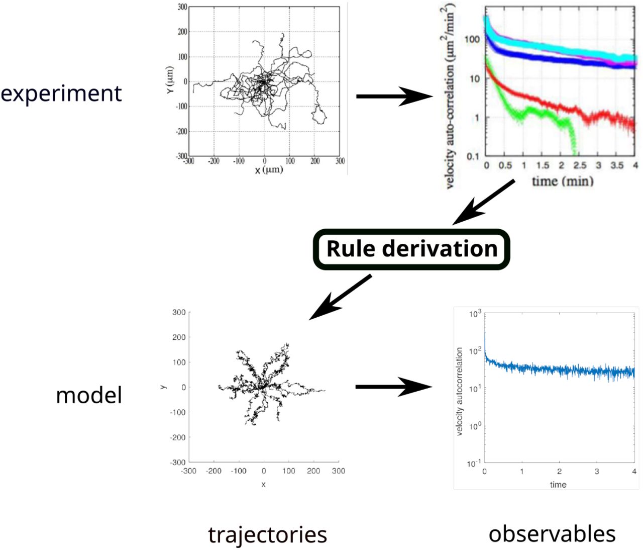
BIO-LGCA modelling with data-driven rules. First, an experiment is performed and data (here: migration trajectories) are gathered. Second, the data is processed and a characteristic observation is selected (here the observation is the velocity autocorrelation function). Third, a BIO-LGCA model is constructed by deriving rules from the experimental observations (see Fig. 4), and data (trajectories) are gathered from simulations. The model can be validated by showing that it reproduces experimental observations (here, the velocity autocorrelation function). Experimental plots of D. discoideum trajectories (top) were adapted from [19]. BIO-LGCA simulation plots of single-cell trajectories (bottom) were produced by the authors from a BIO-LGCA model obtained from experimental plots as described within the main text.
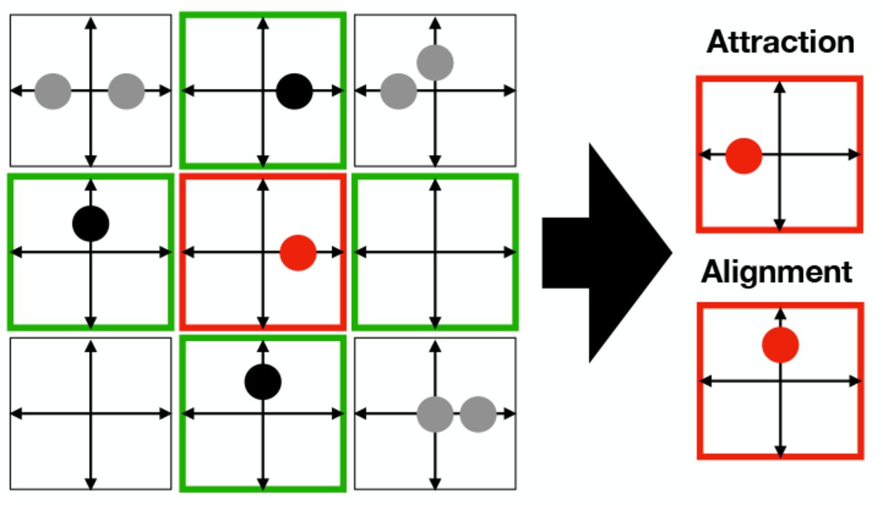
Basic interactions with neighbourhood impact; node configuration (red) before and after application of stochastic interaction rule: cell-cell attraction (top), cell alignment (bottom).
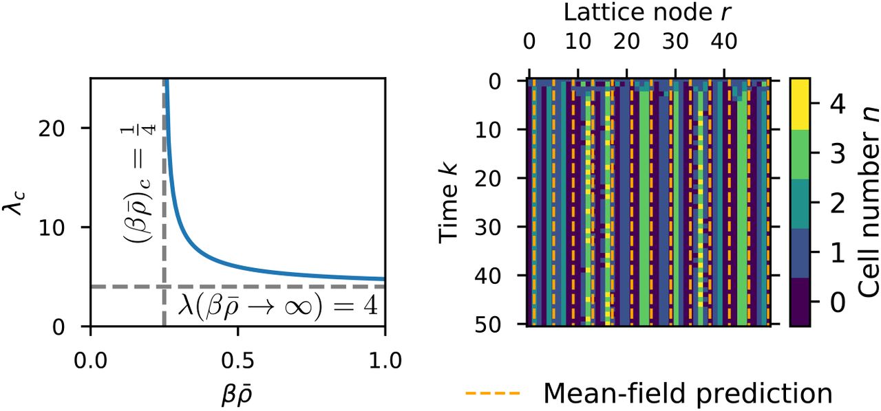
Pattern formation in the LGCA aggregation rule. Left: critical wave length obtained from the mean-field analysis. The critical wave length diverges for  , and
, and  Right: emergence of a periodic pattern from a homogeneous initial state. The horizontal distance of the orange dashed lines is equal to the critical wave length predicted by mean-field analysis. Parameters: β = 100,
  , a = 2.
Collective migration
Let’s now consider the case where the reorientation potential is of the form
 that is, the reorientation potential depends only on the cosine of the orientation of the central cell, whose amplitude and shift may depend on the positions and/or orientations of all cells within the neighbourhood of interaction (including the central cell) only through the amplitude (C) and shift (φ) of the cosine writfunction. Using trigonometric identities, the reorientation potential can then be rewritten as
 where G({xk}, {θk}) is called the local director field, whose norm and argument are, respectively, ‖G({xk}, {θk})‖ = C({xk}, {θk}) and arg[G({xk}, {θk})] = φ ({xk}, {θk}). Substituting Eq. 10 in Eq. 8, and using the linearity of the internal product, the transition probability of the reorientation operator is
 where
where  is the local director field of the neighbourhood configuration, and J(s) is the node flux, as described previously.
In general, whenever the reorientation potential can be expressed as
 with n ∈ ℕ, the argument of the exponential in the transition probability can be expressed as an internal product of two vectors. In the specific case of n = 2, using trigonometric functions, one can arrive at the transition probability
 where N(s) is the local nematic alignment vector, and is defined as

Thus, the reorientation probabilities have the same general form whenever the interaction potential is conservative and consists of a pairwise comparison between the angles and/or positions of neighbouring cells.
5.2 Data-driven rules
Due to the complexity of inter- and intracellular processes, it is not uncommon to have little knowledge about biophysical mechanisms mediating single and collective cell migration. Typically, there is partial to no knowledge of the intracellular processes underlying experimental observations, such as signalling pathways. In this case, statistical methods can be used to derive reorientation rules needed to define appropriate BIO-LGCA models.
Suppose that an experimental observation is the only known information about a single or collective cell migration process, with no knowledge about the underlying mechanisms driving such process. These observations are typically averages of a time-dependent quantity (called the observable). The reorientation probabilities of the corresponding BIO-LGCA model should be chosen such that the mean of the observable function matches the experimental observation. For example, a common observable is the comparison between the initial cell velocity v0, and the velocity at a later time t, vt, expressed as v0 vt. The corresponding experimental observation is called the velocity autocorrelation function, defined as g(t) = 〈v0 · vt〉.
However, this is not enough to completely determine the probability distribution. Take, for example, a zero-mean observation. Most symmetric distributions centered about zero will fulfill the observation. Which functional form of the probabilities to choose, then? We can actually exploit the lack of information on the mechanistic nature of the process to our own advantage. The maximum caliber (and maximum entropy) formalism [18] dictates to maximise entropy (a measure of the lack of information contained in a probabilistic model) while restricting probabilities to reproduce the experimental observation. This translates into optimising the following functional
 where PΓ is the probability of a cellto follow a certain spatial trajectory Γ, β(j) and λ are Lagrange multipliers,
  is the value of the observable at the time step k depending on the state of the lattice
  , and Ek is the value of the observation at the time step k, which is the average of the observable obtained from experimental data. The first term of the functional is the entropy, which we want to maximise. The second term restricts the resulting probabilities to match the experimental observation. Since we assume the observation, Ek to be a time-dependent function, then a Lagrange multiplier β(k) is needed for every time step k. The last term guarantees the normalisation of probabilities, which requires and additional Lagrange multiplier, λ.
The optimisation of this functional yields an optimal value for the path probabilities  , where the value of β(j) is such that
  .
.
If the process is Markovian, then one may decompose the path probability into individual channel occupation probabilities for each time step k, as
 where the observable is dependent on the occupancy of the i-th channel of the node and conditioned to a certain configuration of its interaction neighbourhood. For example, if the observation is the autocorrelation function g(t) = 〈v0 · vt〉, where vt denotes the normalized velocity of a cell at the time t, determined from experimental data, then the corresponding channel occupation probabilities are found to be
 where z is the normalisation constant for the transition probability, d is the dimension of space, and
  is the initial orientation of the cell.
If we assume independence among cells within the same node, we arrive at a reorientation probability of the form

Note that, if both observation and observable are time-independent, then the Lagrange multiplier β(k) = β is also time independent, and the transition probabilities are given by


6 BIO-LGCA rules for single and collective cell migration
Now that the BIO-LGCA framework has been defined and data- and equation-based methods for rule derivation have been described, we present key examples of transition probabilities corresponding to reorientation operators, which model important elementary single-cell and collective behaviours. Note that several of these examples’ probabilities have the general form of Eq. 11.
6.1 Single cell migration
Random walk
Random walks are performed by cells such as bacteria and amoebae in the absence of any environmental cues. Random walk of cells can be modeled by a reorientation operator with the following transition probabilities:

This rule conserves mass, i.e. cell number.
Chemotaxis
Chemotaxis describes the dependence of individual cell movement on a chemical signal gradient field. Accordingly, spatio-temporal pattern formation at the level of cells and chemical signals can be observed. Chemotactic patterns result from the coupling of different spatio-temporal scales at the cell and the molecular level, respectively.
To mimick a chemotactic response to the local signal concentration, we define the signal gradient field
 where
where  . Chemotaxis can be modeled through a reorientation operator with transition probabilities given by
 where β is the chemotactic sensitivity of the cells.
With large probability, cells will move in the direction of the external chemical gradient Gsig.
Haptotaxis
We consider cell migration in a static environment that conveys directional information expressed by a vector field

A biologically relevant example is haptotactic cell motion of cells responding to fixed local concentration differences of adhesion molecules along the extracellular matrix (ECM). In this example, the local spatial concentration differences of integrin ligands in the ECM constitute a gradient field that creates a “drift” E[20].
The transition probabilities associated to the reorientation operator, given a vector E ∈ ℝ2, is given by
 where E ∈ ℝ2.
In this case, cells preferably move in the direction of the external gradient E.
Contact guidance
We now focus on cell migration in environments that convey orientational, rather than directional, guidance. Examples of such motion are provided by neutrophil or leukocyte movement through the pores of the ECM, the motion of cells along fibrillar tissues, or the motion of glioma cells along fiber track structures. Such an environment can be represented by a second rank tensor field that encodes the spatial anisotropy along the tissue. In each point, the corresponding tensor informs the cells about the local orientation and strength of the anisotropy and induces a principal (local) axis of movement. Thus, the enviroment can again be represented by a vector field

Contact guidance can be modeled through a reorientation operator with transition probabilities defined as

6.2 Collective cell migration
Several kinds of organisms, as well as biological cells, e.g. fibroblasts, can align their velocities globally through local interactions. Here, we introduce a reorientation operator where the local director field is a function of the states of several channels and nodes, reflecting the influence of neighbouring cells during collective cell migration.
 where
where  is the local cell momentum This particular reorientation probability triggers cell alignment [21].
6.3 Attractive interaction
Biological cells can interact via cell-cell adhesion, through filpodia cadherin interaction, for example. Agent attraction/adhesion can be modeled with a reorientation operator with the following probability distribution.
 where
where  is the density gradient field.
This reorientation probability favors cell agglomeration. A similar rule has been introduced in [22].
7 Mean-field analysis
We here demonstrate the mean-field analysis of the BIO-LGCA for the example of the attractive interaction eq. (24). This analysis allows to predict collective behaviour. In particular, we calculate the critical sensitivity βc, such that aggregation occurs for β > βc, while a homogeneous initial conditions is stable for β < βc. Under “mean-field” we here understand that we neglect correlations between the occupation numbers of different channels and that we approximate the mean value of any function f of a random variable X by the function evaluated at the mean value of the random variable, i.e. 〈f(X)〉 ≈ f(〈X〉). As we are interested in the onset of aggregation from a homogeneous initial state with low density  and weak interaction β ⪡ 1 we can linearize the transition probabilities. We further assume that there is at most one cell at each node and therefore only consider single-cell transitions (n = 1). For the partition function Z we then obtain
 due to the symmetry of the lattice. For the single-cell transition probability we obtain

Since the transition probability only depends on the number of cells on the neighbouring nodes, but not on their distribution on the channels, we analyze the mean local density

According to the propagation rule the cell number n(r, k + 1) is given by

We calculate the expected value under the mean-field assumption in terms of numbers of cells n(r) at node  , and the number of cells
  in the neighbourhood of
  as
as

As in the low-density regime  , we can use the single-cell transition probability eq. (26) and the factorizing probability distribution under our meanfield assumption to obtain

To proceed, we assume a one-dimensional lattice, where b = 2, c1,2 = ± 1 with a rest channels to obtain the finite-difference equation (FDE)

This FDE can be analyzed by means of linear stability analysis. To do this, we first rewrite eq. (31) in terms of the density difference Δρ(r, k) := ρ(r, k + 1) ρ(r, k), which we linearize around the steady state for a small perturbation of the form 


We now apply the discrete Fourier transform
 and obtain the mode-dependent FDE

 using 2cosx = eix + e−ix and cos2x = 2cos2 x − 1. Note that the system becomes unstable when the r.h.s. of the equation is larger than 0, meaning the perturbation grows, while it is stable with a decreasing perturbation if it is smaller than 0. To find the dominant Fourier mode q that maximizes the r.h.s. we assume an infinite lattice L → ∞ so that we can define the quasicontinuous wave number
  and use the derivative with respect to κ to calculate the maxima of the bracket on the r.h.s. of eq. (36),


Note that we divided by sin κ here, neglecting the trivial solutions κ = 0, π. Clearly the solution  is only valid for
  it is the dominant wave number in this case. This in turn allows us to define the critical parameter combination
  . We can also calculate the dominant wave length in dependence of
  as
as  , which diverges at
  and approaches λc → 4 for
  .
.
8 Discussion
In contrast to “continuumsystems” and their canonical description with partial differential equations, there is no standard model for describing interactions of discrete objects, particularly interacting discrete biological cells. In this paper, the BIO-LGCA is proposed as a lattice-based model class for a spatially extended system of interacting cells. The BIO-LGCA idea can be expanded to multispecies models with different cell phenotypes where cell phenotypes may differ in their migration or interaction behaviours reflected in the specific interaction rule (cp. also [23]). It is also possible to extend the BIO-LGCA idea to heterogeneous populations and environments, e.g. cells which differ in their adhesivities and/or which interact with a heterogeneous non-cellular environment [24, 25]. BIO-LGCA models are appropriate for low and moderate cell densities. For higher densities e.g. in epithelial issues, cell shape may mat-ter and other models, such as the Cellular Potts model, may be better choices (see [2, 26] for reviews of on- and off-lattice models). It is also important to be aware of lattice artefacts inherent to the spatial discretization considered in every cellular automaton model, e.g. the checkerboard artefact (cp. [27]). In two spatial dimensions, the hexagonal lattice possesses less artefacts than the square lattice. A major advantage of BIO-LGCA models compared to other on-and off-lattice cell-based models for interacting cell systems, such as interacting particle systems, e.g. [28, 29], asynchronous cellular automata, e.g. [30, 31, 32], further cell-based models [33] or systems of stochastic differential equations [34], is their computational efficiency, and their synchronicity and explicit velocity consideration, which enables the modeling of moderately packed cell collectives while minimizing model artifacts.
Most BIO-LGCA models do not conserve momentum, especially if they model active cells in highly viscous environments and spend energy to bypass momentum conservation. In particular, cell motion may be influenced by the interaction of cells with components of their microenvironment through haptotaxis or differential adhesion, contact guidance, contact inhibition, and processes that involve cellular responses to signals that are propagated over larger distances (e.g. chemotaxis). BIO-LGCA models have already been used in the study of several biological processes, namely angiogenesis [35], bacterial rippling [36], Turing pattern formation [37], active media [38], epidemiology [39] and various aspects of tumor dynamics [24, 40, 41, 42, 43, 44, 45, 46, 47], among others.
BIO-LGCA models allow multiscale analysis of behaviours emerging at multiple temporal and spatial scales. The microscopic scale is much smaller than the typical cell size and is not explicitly considered in BIO-LGCA models. The macroscopic scale is much larger than the cell size and refers to the behaviour of the cell population. Thus, a BIO-LGCA operates at a mesoscopic scale between the microscopic and the macroscopic scale: the mesoscopic scale coarse-grains microscopic properties but distinguishes individual cells. BIO-LGCA as “mesoscopic” models can be regarded either as coarse-grained microscopic models, or discretized macroscopic models. The BIO-LGCA framework facilitates theoretical analysis of emergent, tissue-scale (macroscopic) behaviours [27]. In many cases, the macroscopic behaviour of the mesoscopic BIO-LGCA can be analyzed using reasonable approximations, such as through a spatial mean-field description based on a partial differential equation [27, 48, 49, 50] (see also sec. 7). In particular, BIO-LGCA have been used for analysing collective behaviours at the macroscopic biological tissue level that result from local cellular interactions. Typical examples of observables at a macroscopic scale are cell density patterns and quantities related to the dynamics of moving cell fronts and cluster size distributions [51, 52, 53]. Cell density patterns can often be assessed experimentally and provide, therefore, a means to relate BIO-LGCA model predictions to experimental observations.
Meanwhile, microscopic model descriptions in the form of stochastic differential equations have been derived from a mesoscopic individual-based BIO-LGCA formulation as well [54]. Note that in standard LGCA and BIO-LGCA individual agents can not be distinguished and therefore followed.
The BIO-LGCA modeling strategy is “modular”: starting from “basic models”, which include those explored in this paper such as alignment, contact guidance/repulsion, hapto- and chemotaxis. Coupling them is required to design models for complex biological problems. The focus of future activities is the analysis of further model combinations for selected biological problems, which are not necessarily restricted to cells but could also comprise interactions at subcellular and tissue scales. The resulting multi-scale models will contain a multitude of coupled spatial and temporal scales and will impose significant challenges for their analytic treatment.
10 Acknowledgments
HH gratefully acknowledges the funding support of the Helmholtz Association of German Research Centers—Initiative and Networking Fund for the project on Reduced Complexity Models (ZT-I-0010). HH is supported by MulticellML (01ZX1707C) of the Federal Ministry of Education and Research (BMBF) and the Volkswagenstiftung within the “Life?” programm (96732). A.D. acknowledges support by the EU-ERACOSYS project no. 031L0139B. The authors thank the Centre for Information Services and High Performance Computing at TU Dresden for providing an excellent infrastructure.
Footnotes

References
- [1].↵
- [2].↵
- [3].↵
- [4].↵
- [5].↵
- [6].↵
- [7].↵
- [8].↵
- [9].↵
- [10].↵
- [11].↵
- [12].↵
- [13].↵
- [14].↵
- [15].↵
- [16].↵
- [17].↵
- [18].↵
- [19].↵
- [20].↵
- [21].↵
- [22].↵
- [23].↵
- [24].↵
- [25].↵
- [26].↵
- [27].↵
- [28].↵
- [29].↵
- [30].↵
- [31].↵
- [32].↵
- [33].↵
- [34].↵
- [35].↵
- [36].↵
- [37].↵
- [38].↵
- [39].↵
- [40].↵
- [41].↵
- [42].↵
- [43].↵
- [44].↵
- [45].↵
- [46].↵
- [47].↵
- [48].↵
- [49].↵
- [50].↵
- [51].↵
- [52].↵
- [53].↵
- [54].↵


