Utility of polygenic embryo screening for disease depends on the selection strategy

Abstract

As of 2019, polygenic risk scores have been utilized to screen in vitro fertilization embryos for genetic liability to adult diseases, despite a lack of comprehensive modeling of expected outcomes. In this short report, we demonstrate that a strong determinant of the potential utility of such screening is the selection strategy employed, a factor that has not been previously studied. Minimal risk reduction is expected if only extremely high-scoring embryos are excluded, whereas risk reductions are substantially greater if the lowest-scoring embryo (for a given disease) is selected. We systematically examined the relative contributions of the variance explained by the score, the number of embryos, the disease prevalence, and parental scores and disease status on the utility of screening. We discuss the results in the context of relative vs absolute risk, as well as the potential ethical concerns raised by such procedures.

Introduction

Polygenic risk scores (PRS) have become increasingly well-powered, relying on findings from large-scale genome-wide association studies for numerous diseases (Visscher et al., 2017; Wray et al., 2013). The predictive power of a PRS is usually represented by R² (or, as we denote it below, ), the proportion of variance of the liability of the disease explained by the score (Dudbridge, 2013). However, for potential clinical applications, this statistical property needs to be translated into clinically actionable information (Torkamani et al., 2018). This translation requires careful consideration of the specific purposes for which the PRS will be used. For example, individuals with polygenic scores in the top percentiles for coronary artery disease (CAD) were shown to be as likely to have a heart attack as individuals heterozygous for a familial hypercholesterolemia mutation (Khera et al., 2018), and may therefore be good candidates for preventative treatment. By contrast, a wider range of high PRS scores (e.g, top quartile), may provide useful information as a part of a multimodal screening process for cancer risk (Callender et al., 2019; X. Zhang et al., 2018).

Another potential clinical application of PRSs is preimplantation screening of in vitro fertilization (IVF) embryos. Although currently in use (Treff, Eccles, et al., 2019) and fraught with ethical concerns (Lázaro-Muñoz et al., 2020), “polygenic embryo screening” (PES) has not yet received much research attention from either geneticists or ethicists. Understanding the statistical properties of PES forms a critical foundation to ethical consideration of the practice (Lázaro-Muñoz et al., 2020). For example, we have recently demonstrated that screening embryos on the basis of polygenic scores for quantitative traits (such as height or intelligence) has limited predictive power in most realistic scenarios (Karavani et al., 2019), and that is a more significant determinant of PES utility for quantitative traits compared with the number of available embryos (n). On the other hand, a series of four studies (Lello et al., 2020; Treff, Eccles, et al., 2019; Treff et al., 2020; Treff, Zimmerman, et al., 2019) conducted by a private company providing embryo screening services has suggested that PES for dichotomous disease risk may have significant clinical utility. However, these studies examined a relatively limited range of scenarios, primarily focusing on distinctions between sibling pairs discordant for illness, and did not provide a comprehensive examination of the potential utility of PES.

Here, we use statistical modeling to examine the potential utility of PES for disease risk (defined in terms of relative and absolute risk reduction), comparable to our prior study of PES for quantitative traits (Karavani et al., 2019), with an aim toward informing future ethical deliberations on the practice. We study a range of realistic scenarios, quantifying the role of , the number of embryos (n), the disease prevalence, and parental risk scores and disease status on the ability of PES to reduce disease risk when screening for a single disease (Materials and Methods). We utilize the liability threshold model (Falconer, 1967) to represent disease risk as a continuous liability, comprising genetic and environmental risk factors, under the assumption that individuals with liability exceeding a threshold are affected. The liability threshold model was shown to be consistent with data from family-based transmission studies (Wray & Goddard, 2010) and GWAS data (Visscher & Wray, 2015). Consequently, we define the disease risk of a given embryo probabilistically, as the chance that its liability will cross the threshold at any point after birth (Figure 1A).

Figure 1. A schematic of the liability threshold model and polygenic embryo screening.

(A) An illustration of the liability threshold model (LTM). Under the LTM, it is assumed that each disease has an underlying (unobserved) liability, and that an individual is affected if the total liability is above a threshold. The liability is composed of a genetic component and an environmental component, both assumed to be normally distributed in the population. For a given genetic risk (represented here by the polygenic risk score), the liability is the sum of that risk, plus a normally distributed residual component (environmental + genetic factors not captured by the PRS). Thus, for an individual with high genetic risk (bottom curve), even a modestly elevated (and thus, commonly-occurring) liability-increasing environment will lead to disease. For an individual with low genetic risk (top curve), only an extreme environment will push the liability beyond the disease threshold, making the disease less probable. Thus, disease risk reduction can be achieved with embryo screening by lowering the genetic risk of the implanted embryo. [Note that for the purpose of illustration, panel A displays three discrete levels of genetic risk, although in reality PRS is continuously distributed.] (B) An illustration of the embryo selection strategies considered in this report. In the figure, each embryo is shown as a filled circle, and embryos are sorted based on their predicted risk, i.e., their polygenic risk scores. Excluded embryos are shown in pink, and embryos that can be implanted in green. The risk reduction (RR) is indicated as the difference in risk between a randomly selected embryo (if no polygenic scoring was performed) and the embryo selected based on one of two strategies. In high-risk exclusion (HRE), the embryo selected for implantation is random, as long as its PRS is under a high-risk cutoff (usually the top few PRS percentiles). If all embryos are high-risk, a random embryo is selected. In lowest-risk prioritization (LRP), the embryo with the lowest PRS is selected for implantation. As we describe below, the LRP strategy yields much larger disease risk reductions.

In studies of potential clinical utility of PRSs in adults, attention has focused on those in the highest percentiles of risk, in which odds ratios become sufficiently large to be clinically meaningful (Chatterjee et al., 2016; Dai et al., 2019; Gibson, 2019; Khera et al., 2018; Mars et al., 2020; Mavaddat et al., 2019; Torkamani et al., 2018). To our knowledge, PES is currently being employed in a similar fashion, following a strategy of excluding embryos with extremely high (top 2-percentiles) PRS (Treff, Eccles, et al., 2019; Treff et al., 2020), which we term “high-risk exclusion” (HRE: Figure 1B, upper panel). In such a strategy, after high-risk embryos are set aside, an embryo is randomly selected for implantation among the remaining available embryos. (In the rare scenario that all embryos are high-risk, we assume a random embryo is selected among them.) We utilized both theory and simulations to study this strategy, given varying disease prevalence, strength of PRS, and embryo exclusion thresholds. As elaborated below, we demonstrate that the HRE strategy has very limited utility, but that a strategy of selecting the embryo with the lowest genetic risk can result in large risk reductions.

Results and Discussion

We quantified the outcome of PES in terms of relative risk reduction (RRR), defined as , where K is the prevalence. For example, if a disease has prevalence of 5% and the selected embryo has a probability of 3% to be affected, the relative risk reduction is 40%. The achievable risk reductions with the high-risk exclusion strategy (Materials and Methods) are plotted in Figure 2 (upper row), showing strong dependence on the PRS exclusion threshold. When the 2-percentile threshold is applied (straight black lines), the reduction in risk is limited; RRR is <10% in all scenarios where . Currently, is the upper limit of predictive power (on the liability scale) of PRS for most complex diseases (Khera et al., 2018; Lambert et al., 2019), with the exception of a few disorders with large-effect common variants (such as Alzheimer’s disease or type 1 diabetes) (Sharp et al., 2019; Q. Zhang et al., 2020).

Figure 2. The relative risk reduction across selection strategies and disease parameters.

The relative risk reduction (RRR) is defined as (K – P(disease))/K, where K is the disease prevalence, and P(disease) is the probability of the implanted embryo to become affected. The RRR is shown for the high-risk exclusion (HRE) strategy in the upper row (panels A-C), and for the lowest-risk prioritization (LRP) in the lower row (panels D-F). See Figure 1 for the definitions of the strategies. Results are shown for values of K = 1%, 5%, 20% in each panel, and within each panel, for variance explained by the PRS (on the liability scale) (legends). Symbols denote the results of Monte-Carlo simulations (Materials and Methods), where PRSs of embryos were drawn based on a multivariate normal distribution, assuming PRSs are standardized to have zero mean and variance , and accounting for the genetic similarity between siblings (Eq. (4) in Materials and Methods). In each simulated set of n sibling embryos (n = 5 for all simulations under HRE), one embryo was selected according to the selection strategy. The liability of the selected embryo was computed by adding a residual component (drawn from a normal distribution with zero mean and variance 1 – ) to its standardized polygenic score. The embryo was considered affected if its liability exceeded z_K, the (upper) K-quantile of the standard normal distribution. We repeated the simulations over 10⁶ sets of embryos and computed the disease risk. In each panel, curves correspond to theory: Eq. (31) in Materials and Methods for the HRE strategy, and Eq. (20) in Materials and Methods for the LRP strategy. Black straight lines correspond to the RRR achieved when excluding embryos at the top 2% of the PRS (for HRE, upper panels) or for selecting the lowest risk embryo out of n = 5 (for LRP, lower panels).

In the future, more accurate PRSs are expected; however, it has been suggested that , which is at the top end of the common-variant SNP heritability for even the most heritable diseases such as schizophrenia and celiac disease (Holland et al., 2020; Y. Zhang et al., 2018), is the maximal realistic value for the foreseeable future (Wray et al., 2020). At this value, relative risk reduction would only be 20% for K = 0.01, 9% for K = 0.05, and 3% for K = 0.2. These small gains achieved with high-risk exclusion follow because the overwhelming majority of affected individuals do not have extreme scores (Murray et al., 2020; Wald & Old, 2019).

Risk reduction increases as the threshold for exclusion is expanded to include the top quartile of scores, and then reaches a maximum at ≈25-50% under a range of prevalence and values. For all of these simulations, we set the number of available embryos to n = 5, which is a reasonable estimate of the number of testable, viable embryos from a typical IVF cycle (Sunkara et al., 2011). Simulations show that these estimates do not change much with increasing the number of embryos (see Figure 2 - Figure Supplement 1). This holds especially at more extreme threshold values, since most batches of n embryos will not contain any embryos with a PRS within, e.g., the top 2-percentiles.

Figure 2 - Figure Supplement 1. The relative risk reduction for the high-risk exclusion strategy, with n = 10 available embryos.

All details are exactly as in panels (A-C) in Figure 2 of the main text, except that we simulated n = 10 embryos.

The high-risk exclusion strategy treats non-high-risk embryos equally; however, other strategies are possible. For example, current research on optimizing IVF protocols focuses on ranking embryos for potential viability, on the basis of microscopy and time-lapse imaging (Bormann et al., 2020; Montag et al., 2013; Rhenman et al., 2015). Thus, it is readily conceivable that the ranking of embryos on the basis of disease PRS could also be attempted. We term the implantation of the embryo with the lowest PRS as “lowest-risk-prioritization” (LRP; Figure 1b, lower panel). As we show in Figure 2 (lower panels), for LRP with n = 5 available embryos, RRR>20% across the entire range of prevalence and parameters considered, and can reach ≈50% for K ≤ 5% and , and even ≈80% for K = 1% and . While RRR continues to increase as the number of available embryos increases, the gains are quickly diminishing after n = 5.

We also examined the effects of parental PRSs on the achievable risk reduction, given the possibility that families with high genetic risk for a given disease would be more likely to seek PES. Figure 2 - Figure Supplement 2 demonstrates that, as expected, the HRE strategy shows greater relative risk reduction as parental PRS increases, in particular when excluding only very high-scoring embryos. In contrast, the RRR for the LRP strategy is relatively stable across parental PRSs. Nevertheless, as expected, the RRR for the LRP strategy remains greater than that for the HRE strategy across all possible combinations of parameters. Similarly, it is possible that families may be more likely to seek PES when one or both prospective parents is affected by a given disease. Figure 2 - Figure Supplement 3 illustrates that parental disease status has relatively little impact on the expected risk reduction, especially in comparison to conditioning on the parental polygenic risk scores. This is because, as long as , parental disease does not necessarily provide much information about parental PRS, and thus does not strongly constrain the number of risk alleles available to each embryo.

Figure 2 - Figure Supplement 2. The relative risk reduction when the polygenic risk scores of the parents are known.

Panels (A)-(D) are for the high-risk exclusion (HRE) strategy, while panels (E)-(H) are for the lowest-risk prioritization (LRP) strategy. All details are as in Figure 2 of the main text, except the following. First, we fixed the prevalence at K = 5%. Second, in the simulations, we drew the PRS of each embryo as s_i = x_i + c (i = 1, …, n), where x_i is an embryo-specific component (independent across embryos) and c is the shared component, also representing the mean parental PRS (Materials and Methods). This is so far as in Figure 2; however, here we assumed that c is given, equal to the average PRSs of the two parents. In each panel, we consider a different pair of PRSs for the parents. For example, in panels (A) and (E), both parents (“par. 1” and “par. 2”) have PRS equal to the 50% percentile of the PRS distribution; in panels (B) and (F), one parent has PRS equal to the 98% percentile of the PRS distribution, while the other has PRS equal to the 25% percentile; and so on. Third, in the simulations, we computed the risk reduction (according to either strategy) relative to a baseline, obtained from the same sets of simulations, when we always selected the first embryo. The baseline risk is indicated in each legend as “bl”. Note that the baseline risk depends on the variance explained by the PRS, because the parental PRSs are determined as percentiles of the population distribution of the score, which has variance . Finally, we computed the theoretical disease risk for the HRE strategy using Eq. (29) from Materials and Methods, the disease risk for the LRP strategy using Eq. (23), and the relative risk reduction (shown in curves) for both strategies using Eq. (36).

Figure 2 - Figure Supplement 3. The relative risk reduction when the parental disease status is known.

Panels (A)-(C) are for the high-risk exclusion (HRE) strategy, while panels (D)-(F) are for the lowest-risk prioritization (LRP) strategy. The details are as in Figure 2 of the main text, except the following. First, we fixed the prevalence at K = 5% and the heritability to h² = 0.4 (note that the heritability was not needed in previous figures). Second, in the simulations, we first drew the parental genetic components: s_m and w_m for the mother, and s_f and w_f for the father, where are the polygenic scores and represent the non-score genetic factors (Materials and Methods). We drew the environmental component for each parent as ∊_m ~ ∊_f ~ N(0,1 − h²) and computed the liability of each parent as s + w + ∊. If the liability of a parent exceeded Z_K (the (1 − K)-quantile of the standard normal distribution), we designated that parent as affected. We then stratified the risk reduction results based on the number of affected parents: 0 (panels (A) and (D), 1 (panels (B) and (E)), and 2 (panels (C) and (F)). Note that as expected, the number of families in which both parents are affected is small, and thus, the results in panels (C) and (F) are noisier. For each set of parents, we drew the PRS of each embryo as s_i = (s_m + s_f)/2 + x_i (i = 1, …,n), where is an embryo-specific component of the score (independent across embryos). We then selected one embryo from each family based on either selection strategy. We computed the liability of the selected embryo as s_i + (w_m + w_f)/2 + v_i + ∊_i, where is the embryo specific component of the non-score genetic factors, and ∊_i ~ N(0,1 − h²) is the environmental component of the embryo (Materials and Methods). The embryo was designated as affected or unaffected as described above for the parents. We computed the risk reduction (according to either strategy) relative to a baseline, obtained from the same sets of simulations when we always selected the first embryo. The baseline risk is indicated on top of each panel. We computed the theoretical relative risk reduction for the two strategies as summarized in Section 7.9 of the Materials and Methods.

It is important to emphasize that all of the above results are presented in terms of relative risk reduction. The clinical interpretation of these changes in terms of absolute risk will vary based on the population prevalence of the disorder (or the baseline risk of specific parents), and can offer a very different perspective on the magnitude of the effects (Figure 2 - Figure Supplement 4) (Gordis, 2014; Lázaro-Muñoz et al., 2020; Murray et al., 2020). Specifically, a large relative risk reduction may result in a very small change in absolute risk for a rare disease. As an example, schizophrenia is a highly heritable (Sullivan et al., 2003) serious mental illness with prevalence of at most 1% (Perälä et al., 2007). The most recent large-scale GWAS meta-analysis for schizophrenia (Schizophrenia Working Group of the Psychiatric Genomics Consortium, 2020) has reported that a PRS accounts for approximately 8% of the variance on the liability scale. Our model shows that a 52% RRR is attainable using the LRP strategy with n = 5 embryos. However, this translates to only ≈0.5 percentage points reduction on the absolute scale: a randomly-selected embryo would have a 99% chance of not developing schizophrenia, compared to a 99.5% chance for an embryo selected according to LRP. In the case of a more common disease such as type 2 diabetes, with a lifetime prevalence in excess of 20% in the United States (Geiss et al., 2014), the RRR with n = 5 embryos (if the full SNP heritability of 17% (Y. Zhang et al., 2018) were achieved) is 43%, which would correspond to >8 percentage points reduction in absolute risk.

Figure 2 - Figure Supplement 4. The absolute risk reduction when the polygenic risk scores of the parents are known.

All details are the same as in Figure 2 - Figure Supplement 2, except that the absolute (rather than the relative) risk reduction is shown. The absolute risk reduction is defined as the difference between the baseline disease risk (given the parental PRSs; legends) and the risk following either strategy of embryo selection. It is plotted as percentage points.

The results of the present study demonstrate that, contrary to our previous study of PES for quantitative traits (Karavani et al., 2019), substantial effects of PES for disease risk are attainable under certain conditions. Specifically, we observed that the selection strategy is a crucial determinant of risk reduction. The use of PRS in adults has focused on those at highest risk (Chatterjee et al., 2016; Dai et al., 2019; Gibson, 2019; Khera et al., 2018; Mars et al., 2020; Mavaddat et al., 2019; Torkamani et al., 2018), for whom there may be maximal clinical benefit of screening and intervention. However, as PRSs have relatively low sensitivity, such a strategy is relatively ineffective in reducing the overall population disease burden (Ala-Korpela & Holmes, 2020; Wald & Old, 2019). Similarly, in the context of PES, exclusion of high-risk embryos will result in relatively modest risk reductions.

The differential performance of PES across selection strategies and risk reduction metrics may be difficult to communicate to couples seeking assisted reproductive technologies (Cunningham et al., 2015; Wilkinson et al., 2019). These difficulties are expected to exacerbate the already profound ethical issues raised by PES (as we have recently reviewed (Lázaro-Muñoz et al., 2020)), which include stigmatization (McCabe & McCabe, 2011), autonomy (including “choice overload” (Hadar & Sood, 2014)), and equity (Sueoka, 2016). In addition, the ever-present specter of eugenics (Lombardo, 2018) may be especially salient in the context of the LRP strategy. We thus call for urgent deliberations amongst key stakeholders (including researchers, clinicians, and patients) to address governance of PES and for the development of policy statements by professional societies. We hope that our statistical framework can provide an empirical foundation for these critical ethical and policy deliberations.

The present study has several limitations. First, our analytical modeling is based on several simplifying assumptions; as we discuss in the Materials and Methods, we do not expect these assumptions to substantially impact the risk reduction estimates, although our estimates likely represent an upper bound relative to real-world scenarios. For example, we did not model the role of family-specific environmental factors (Wang et al., 2017), including the influence of parental genetic factors on the child's environment (Kong et al., 2018; Morris et al., 2020; Mostafavi et al., 2020; Young et al., 2019). Additionally, given the fact that polygenic risk scores are often correlated across diseases (Watanabe et al., 2019; Zheng et al., 2017), selecting based on the PRS of one disease may increase or decrease risk for other diseases. In practice, couples may seek to profile an embryo on the basis of multiple disease PRSs simultaneously, which may affect the overall and per-disease outcomes. These more complex questions will be the subject of future work. Finally, for the purposes of our calculations, we assumed represents the realistic accuracy achievable (within-family) in a real-world setting in the target population. However, the accuracy of PRSs may be sub-optimal when applied in non-European populations, across different socio-economic groups, or within siblings (as compared to between unrelated individuals) (Duncan et al., 2019; Mostafavi et al., 2020). Moreover, currently constructed PRSs do not include rare or ultra-rare variants (including copy number variants), which may have greater penetrance than common variants. On the other hand, future developments in PRS construction will likely increase the realized for some diseases. Either way, the analyses presented in this paper cover a broad range of values of likely to be available at present and in the foreseeable future.

1 Materials and Methods

1 Methods summary

Our model for the polygenic risk scores of a batch of n IVF embryos is described in detail below. Brielly, we write the polygenic scores of the embryos as (s₁,…,s_n), where s_i = x_i + c,(x₁,…,x_n) are embryo-specific independent variables with distribution (where is the proportion of variance in liability explained by the score), and c is a shared component with distribution also representing the mean parental score. In each batch, an embryo is selected according to the selection strategy. For lowest-risk prioritization, we select the embryo with the lowest value of s. For high-risk exclusion, we select the first embryo with score s < z_qr_ps, where z_q is the (1 - q)- quantile of the standard normal distribution. (If no such embryo exists, we select the first embryo.) The liability of the selected embryo is computed as y = s + e, where . We designate the embryo as affected if y > z_K, where z_K is the (1 − K)-quantile of the standard normal distribution and K is the prevalence. For each parameter setting, we compute the disease probability as the fraction of batches (out of 10⁶ repeats) in which the selected embryo was affected.

We also compute the disease probability analytically. For lowest-risk prioritization, we derive the disease risk based on the theory of order statistics. For high-risk exclusion, we first condition on the shared component c, and then study separately the case when all embryos are high-risk (have score s > z_qr_ps), in which the distribution of the unique component of the selected embryo (x) is a normal variable truncated from below at z_qr_ps, and the case when at least one embryo has score s < z_qr_ps, in which x is a normal variable truncated from above. We solved the integrals in the final expressions numerically in R. We also provide explicit results for the case when the family-specific component c is known. Finally, if the parental disease status is known, we integrate the disease probability of the selected embryo over the posterior distribution of the parental score and non-score genetic components. For full details and for an additional discussion of previous work and limitations, see the sections below.

2 The liability threshold model

The liability threshold model (LTM) is a classic model in quantitative genetics (Dempster and Lerner, 1950; Falconer, 1965; Lynch and Walsh, 1998), and is also commonly used to analyze modern data (e.g., (Wray and Goddard, 2010; So et al., 2011; Lee et al., 2011, 2012; Do et al., 2012; Hayeck et al., 2017; Weissbrod et al., 2018; Hujoel et al., 2020)). The LTM assumes that a disease has an underlying “liability”, which is normally distributed in the population, and is the sum of two components: genetic and non-genetic (the environment). Further, the LTM assumes an “infinitesimal”, or "polygenic" genetic basis, under which a very large number of genetic variants of small effect combine to form the genetic component. An individual is affected if his/her total liability (genetic + environmental) exceeds a threshold.

Mathematically, if we denote the liability as y, the LTM can be written as where y ~ N(0, 1) is a standard normal variable, g ~ N(0,h²) is the genetic component, with variance equal to the (narrow-sense) heritability h², and ε ~ N(0, 1-h²) is the non-genetic component. In practice, we cannot measure the genetic component, but only estimate it imprecisely with a polygenic risk score, denoted s. Following previous work (So et al., 2011; Lee et al., 2012; Treff et al., 2019; Karavani et al., 2019), we assume that the LTM can be written, similarly to Eq. (1), as where y ~ N(0, 1) as above, , where is the proportion of the variance in liability explained by the score, and is the residual of the regression of the liability on s (and is uncorrelated with s), representing environmental effects as well as genetic factors not accounted for by the score.

An individual is affected whenever his/her liability exceeds a threshold, i.e., y > τ. The threshold is selected such that the proportion of affected individuals is equal to the prevalence K, i.e., τ = z_K, where z_K is the (1-K)-quantile of a standard normal variable. Thus,

The model is illustrated in Figure 1A of the main text.

3 A model for the scores of n IVF embryos

Consider the polygenic risk scores (for a disease of interest) of n IVF embryos of given parents. We assume no information is known about the parents, or, in other words, that the parents are randomly drawn from the population. The scores of the embryos have a multivariate normal distribution, where the means form a vector of n zeros, and the n × n covariance hbfrix is

The diagonal elements of the matrix are simply the variances of the individual scores of each embryo. The off-diagonal elements represent the covariance between the scores of the embryos, who are genetically siblings. Based on standard quantitative genetic theory (Lynch and Walsh, 1998) (see also our previous paper (Karavani et al., 2019)), the covariance between the scores of two siblings is , and hence the off-diagonal elements follow. [The non-score components (the e terms in Eq. (2)) are also correlated, as they represent both genetic and environmental factors. However, this does not affect the results of the present paper. See also Section 9 below.]

As we showed in our previous work (Karavani et al., 2019), the scores can be written as a sum of two independent multivariate normal variables, s = x + c, with where 0_n is a vector of zeros of length n, I_n is the n × n identity matrix, and J_n is the n × n matrix of all ones. The x_i’s and c_i’s have the same marginal distribution, namely normal with mean zero and variance each. However, the x_i’s are independent, whereas c has a constant covariance matrix, which means that the c_i’s are n identical copies of the same random variable,

Thus, for each embryo i = 1,…,n,

3.1 An alternative interpretation: conditioning on the average parental scores

The representation of the score in Eq. (8) can also be interpreted as conditioning on the average score of the parents. To see that, write the maternal score as s_m and the paternal score as s_f, The variables (s_i,s_m,s_f) have a multivariate normal distribution, with

In the above equation, the variances of all scores are equal to . The covariance terms are , as the relatedness between between parent and child is the same as for pairs of siblings. We assume no correlation between the scores of the parents (i.e., no assortative mating, see Section 10 for discussion). We are now interested in the density of s_i given s_m and s_f, Using standard results for multivariate normal distributions, the conditional density of s_i is N(μ, σ²), where, where

Carrying out the matrix calculations, we obtain

Thus, where we defined the shared component as the average parental score. We therefore have the distribution of the score of the child given the average parental score. The variance of c itself at the population is . Thus, across the population, . In a given family, c is the same across all embryos. Thus, Eq. (13) is equivalent to s_i = c + x_i, with and is an embryo-specific component.

An analogous result holds for the total genetic component of the embryo g_i, simply by replacing the variance explained by the heritability h². In other words, if g_m and g_f are the maternal and paternal genetic components, respectively, then

4 The disease risk when implanting the embryo with the lowest risk

We assume next that we select for implantation the embryo with the lowest polygenic risk score for the disease of interest. Our goal will be to calculate the probability of that embryo to be affected. Since s_i = x_i + c, the score of the selected embryo satisfies where we defined x_min = min(x₁,…,x_n)-Denote by i* the index of the selected embryo (x_i* = x_min). The liability of the embryo with the lowest risk is thus where . Consequently,

Therefore, the liability of the selected embryo can be written as a sum of two (independent) variables: x_min, which is the minimum of n independent (zero mean) normal variables with variance each; and , which is a normal variable with (zero mean and) variance .

The distribution of x_min can be computed bs ased on the theory of order statistics,

In the above equation, the probability that the minimum of n variables is greater than x_m is the probability that all variables are greater than x_m. The distribution of each x is normal with zero mean and variance , and hence , where Φ(·) is the cumulative probability distribution (CDF) of a standard normal variable.

We can now compute the probability of the selected embryo to be affected by the disease by demanding that the total liability is greater than the threshold z_K. Conditional on , where in the fourth line we used Eq. (18). Next, denote by the density of and by ϕ(·) for the probability density function of the standard normal variable. Given that ,

In the third line, we changed variables: . Eq. (20) is our final expression for the probability of the embryo with the lowest score to be affected.

4.1 The risk reduction when conditioning on the mean parental score

Consider the case when c is given, or, in other words, that we know the mean parental polygenic score. Let us compute the disease risk in such a case. We start from Eq. (16),

Then, where in the last line we used Eq. (18).

Finally, recalling that , where in the last line we changed variables, . Eq. (23) thus provides the probability of disease when we are given the mean parental score c.

5 The disease risk when excluding high-risk embryos

We now consider the selection strategy in which the embryo for implantation is selected at random, as long as its risk score is not particularly high. Specifically, we assume that whenever possible, embryos at the top q risk percentiles are excluded. When all embryos have high risk, we assume that a random embryo is selected. Let z_q be the (1−q)-quantile of the standard normal distribution. The variance of the score is , and therefore, the score of the selected embryo must be lower than z_qr_ps.

To compute the disease risk in this case, we first condition on the shared, family-specific component c. We later integrate over c to derive the risk across the population. Denote by x_s the value of x for the selected embryo, and for the moment, also condition on x_s, We have,

To obtain P(disease | c), we need to integrate over f(x_s), the density of x_s, In fact, f(x_s) is a mixture of two distributions, depending on whether or not all embryos were high risk. Denote by H the event that all embryos are high risk, and let us first compute the probability of H. Recall that given c, the scores of all embryos, s_i = x_i + c, are independent. The event H is equivalent to the intersection of the independent events s_i > z_qr_ps for i = 1,…,n. Thus, recalling that ,

Given H, we know that all scores were higher than the cutoff, i.e., that x_i > z_qr_ps − c for all i = 1,…,n. An embryo is then selected at random, and again, we recall that the x_i’s are independent. Thus, x_i, the value of x of the selected embryo, is a realization of a normal random variable truncated from below. Specifically, if f_x(·) is the unconditional density of x, then for x_s > z_qr_ps – c,

In the case H did not occur, we select an embryo at random among embryos with score s_i < z_qr_ps, i.e., x_i < z_qr_ps – c. The density of x_s is again, analogously to the above case, a realization of a normal random variable, but this time truncated from above. For x_s < z_qr_ps – c

Using these results, we can write the unconditional density of x_s,

We can now integrate over all x_s, still conditioning on c, and using Eq. (24) and some algebra, where we defined

Eq. (29) provides an expression for the probability of disease given the mean parental score c.

Finally, we can integrate over all c in order to obtain the probability of disease in the population. Recalling that and denoting its density as f(c), and again after some algebra, where we defined

Eq. (31) is our final expression for the probability of an embryo selected randomly among non-high-risk embryos to be affected.

6 The relative risk reduction

Given the prevalence K and the probability of the selected embryo to be affected P(disease), we define the relative risk reduction (RRR) as

For example, if a disease has prevalence of 5% and the selected embryo has probability 3% to be affected, the relative risk reduction is 40%. We use the relative risk reduction defined in Eq. (33) in the main text, where P(disease) is given by Eq. (20) for the lowest-risk prioritization strategy, and by Eq. (31) for the high-risk exclusion strategy. We solve the integrals in these equations numerically in R (see Section 11).

6.1 The relative risk reduction conditional on the mean parental score

In Sections 4 and 5 we computed the probability of disease conditional on the mean parental score c for the two selection strategies (Eqs. (23) and (29)). Let us denote this probability as P_s(disease | c). To compute the relative risk reduction in these cases, we also need the “baseline” risk, i.e., the probability of disease when a random embryo is selected (as in natural procreation). We denote this probability P_r(disease | c). Let us write the liability of a random embryo as where we defined . , and thus, .

The conditional probability of disease is

The relative risk reduction conditional on the mean parental score can be computed as

The absolute risk reduction is defined as P_r(disease | c) - P_s(disease | c).

7 The risk reduction conditional on family history

7.1 Model

Let us rewrite our model for the liability as

Here, w represents all genetic factors not included in the score. It would be important to keep track of this component as it is also inherited, and hence, information on the disease status in the family will be informative on w for both parents and children. As in Section 2, we assume s, w, and ε are independent, , ε ~ N(0, 1-h²), and thus .

We derive the risk reductions in two main steps. First, we assume that the values of s and w are known for each parent, and compute the risk of the embryo under each selection strategy (lowest-risk prioritization, high-risk exclusion, or random selection). Then, we derive the posterior distribution of the parental genetic components given any specific configuration of family history, and integrate over these components to obtain the final risk estimate.

7.2 The risk of the selected embryo given its score

Denote the maternal score as s_m and the paternal score as s_f, and similarly for w_m and w_f and assume they are given. (Also denote g_m = s_m + w + m and g_f = s_f + w_f.) As we explained in Section 3.1, at any child i the distribution of the score s is where c = (s_m + s_f)/2 and . Similarly, the distribution of the non-score genetic component is where .

Given the parental genetic components, we can write the liability of each embryo as, for i = 1,…, n, where ε_i ~ N(0, 1 – h²). All the three random variables in the above equation (x_i, v_i, and ε_i) are independent, and x_i and v_i are independent across embryos. (It is not necessary to specify whether the ε_i are independent.) Denote the event that embryo i is affected as D_i, and condition on the value of x_i for that embryo. The probability of disease is

The last line holds because .

We denote henceforth D_s as the event that the selected embryo is affected. In the next three subsections, we integrate the probability of the disease over all x_i, where the distribution of x_i will vary depending on the selection strategy. This will give us the disease risk given the parental genetic components.

7.3 Selecting the lowest-risk embryo

Denote by x_i* is the embryo-specific component of the embryo with the lowest such component, where these components are distributed across embryos as . We can use the theory of order statistics, as in previous sections, to compute the density of x_i*.

Eq. (41) can now be integrated over all x_i*. After changing variables , we obtain

Note that the final result depends only on g_m and g_f. Thus, Eq. (43) can be integrated over g_m and g_f (according to their distribution given the family disease history) to provide the disease risk probability.

7.4 Excluding high-risk embryos

Here, the density of the score of the selected embryo is given by Eq. (28), which continues to hold, with c = (s_m + s_f)/2.

Integrating over all x_s, following similar steps as in Section 5, we obtain, denoting by D_s the event that the selected embryo is affected, where we defined

Here, Eq. (45) depends on c, g_m, g_f, and they must be integrated over to obtain the final disease probability.

7.5 The baseline risk

To compute the relative risk reduction, we need the baseline risk, i.e., the risk when selecting a random embryo. Here we need not condition on x_s, Thus,

7.6 The disease risk conditional on the parental disease status

In the subsections 7.3, 7.4, and 7.5, we computed the disease probability for the various strategies. For the baseline risk and for lowest-risk prioritization strategy, the risk depended only on g_m and g_f, For the high-risk exclusion strategy, the risk also depended on c. In this section, we compute the posterior probability of these genetic components conditional on the disease status of the parents.

Denote by D_m the indicator variable that the mother is affected (i.e., D_m = 1 is the mother is affected and D_m = 0 otherwise), and similarly define D_f. The risk of the selected embryo conditional on the parental disease status can be written as

Eq. (48) consists of three terms. The first is P(D_s | g_m, g_f, c), which was computed in the previous subsections for the various selection strategies. Note that P(D_s | g_m, g_f, c, D_m, D_f) = P(D_s | g_m, g_f, c), because, given the genetic components of the parents, their disease status does not provide additional information on the disease status of the children (at least under a model where the environment is not shared). The second term is the density of c, which can be sirnilarly written as f(c | g_m, g_f, D_m, D_f) = f(c | g_m, g_f), The third term is the posterior distribution of g_m and g_f given the parental disease status, f(g_m, g_f | D_m, D_f). In the following, we derive the third term and then the second term.

Note that if P(D_s | g_m, g_f, c) = P(D_s | g_m, g_f), as in the case of the baseline risk (Eq. 47) and the lowest-risk prioritization (Eq. (43)), the risk of the selected embryo can be simplified by integrating over c,

7.7 The distribution of the parental genetic factors given family history

First, it is reasonable to assume that given one parent’s disease status, his/her genetic component is independent of the spouse’s disease status or genetic factors. Thus, the posterior distribution can be factored into

We next assume that the parents are equivalent, and thus, their posterior distributions are identical and we focus on a single parent. To derive the posterior distribution f(g_m | D_m) we first need the prior, g_m ~ N(0, h²),

Next, The likelihood that the mother is affected is

Similarly,

Using Bayes’ theorem,

Similarly,

We have thus specified the posterior distribution f(g_m,g_f | D_m,D_f).

7.8 The distribution of the parental mean score given the parental genetic factors

Let us now compute f(c | g_m,g_f). To this end, we note that c, g_m, and g_f have a multivariate normal distribution,

To explain the above equation, recall that and Then,

A similar result holds for the paternal genetic component. To compute the density of c given g_m and g_f, we use standard theory for multivariate normal variables (as in Section 3.1). We can write where and

Carrying out the matrix calculations, we obtain

We have thus specified f(c | g_m,g_f).

7.9 Summary of the computation

In summary, for the high-risk exclusion strategy, the probability of disease of the selected embyro given the parental disease status is given by Eq. (48), with P(D_s | g_m,g_f,c) given in Eq. (45) and f(c | g_m,g_f) in Eq. (58). The conditional probability of disease for the lowest-risk prioritization strategy and for random selection (the baseline risk) is given by Eq. (49), with P(D_s | g_m,g_f) given in Eqs. (43) and Eq. (47), respectively. For all selection strategies, f(g_m,g_f | D_m,D_f) is given by Eqs. (50), (54), and (55), depending the particular family history.

Numerically, computing the baseline disease risk requires two integrals (over g_m and g_f. Computing the risk for the lowest-risk prioritization strategy requires three integrals (over g_m, g_f, and t). Computing the risk for the high-risk exclusion strategy requires four integrals (over g_m, g_f, c and t).

8 Comparison to previous work

In the “gwem” blog (https://www.gwern.net/Embryo-selection), the utility of embryo selection for traits and/or diseases was investigated. For disease risk, a similar model to ours was studied, based on the liability threshold model. However, the model assumed that given the polygenic score, the distribution of the remaining contribution to the liability has unit variance, instead of (the function liabilityThresholdValue therein). Moreover, only numerical results were provided, the high-risk exclusion strategy was not considered, and there was no analysis of the case when the parental scores or disease status are known. Treff et al. (Treff et al., 2019) also employed the liability threshold model to evaluate embryo selection for disease risk. However, they did not consider the high-risk exclusion strategy, and did not compute analytically the risk reduction. They only provided simulation results for the case when a parent is affected based on an approximate model.

9 Simulations

To simulate the outcomes ofembryo selection, we used the representation s_i = x_i + c, where (x₁,…,x_n) are independent normals with zero means and variance , and is shared across all embryos. Thus, for each “family”, we first drew c, then drew n independent normals (x₁,…,x_n), and then computed the score of embryo i as s_i = x_i + c, for i = 1,…,n. The score of the selected embryo was the lowest among then embryos in the lowest-risk prioritization strategy. For the high-risk exclusion strategy, we selected the first embryo with score s < z_qr_ps If no such embryo existed, we selected the first embryo. We then drew the residual of the liability as , and computed the liability as s* + e, where s* is the score of the selected embryo. If the liability exceeded the threshold z_K, we designated the embryo as affected. We repeated over 10⁶ sets of embryos, and computed the disease probability as the fraction of “families” in which the selected embryo was affected. We compute the relative risk reduction using Eq. (33).

For given parental risk scores, we computed c as c = (s_m + s_i)/2. We specified the maternal score as a percentile p_m, such that the score itself was s_m = z_pmr_ps, where z_pm is the p_m percentile of the standard normal distribution. We similarly specified the paternal score. The remaining calculations were as above. For the baseline risk, we used the same data, with the first embryo in each family.

When conditioning on the parental disease status, we first drew the independent parental components: s_m and s_f as normal variables with zero mean and variance ; w_m and w_f with variance ; and ε_m and ε_f with variance 1 - h². We computed the maternal liability as y_m = s_m + w_m + ε_m, and designated the mother as affected if y_m > z_K. We similarly designated the paternal disease status. We then drew the score of each embyro as s_i = c + x_i, where c = (s_m + s_f)/2 (using the already drawn parental scores) and , for i = 1,…,n, are independent across embryos. We selected one embryo based on the selection strategy, as in the previous paragraph. If s* is the score of the selected embryo, we computed the liability of the selected embyro as s* + (w_m + w_f)/2 + v + ε, where and ε ~ N(1 - h²). We designated the embryo as affected if its liability exceeded z_k. We tallied the proportion of affected embryos for each number of affected parents (0,1,2). To compute the baseline risk, we again used the first embryo in each family.

10 Limitations of the model

Our model has a number of limitations. First, our results relies on several modeling assumptions. (1) We assumed an infinitesimal genetic architecture for the disease, which will not be appropriate for oligogenic diseases or when screening the embryos for variants of very large effect. (2) Our model also assumes no assortative mating, which seems reasonable given that for genetic disease risk, correlation between parents is weak (Rawlik et al., 2019), and given that our previous study of traits showed no difference in the results between real and random couples (Karavani et al., 2019). (3) When conditioning on the parental disease status, we assumed independence between the environmental component of the child and either genetic or environmental factors influencing the disease status ofthe parents. Family-specific environmental factors were shown to be insignificant for complex diseases (Wang et al., 2017). The influence of parental genetic factors on the child's environment is discussed in the next paragraph. Both of these influences, to the extent that they are significant, are expected to reduce the degree of risk reduction.

Second, we assumed that the proportion of variance (on the liability scale) explained by the score is , but we did not specify how to estimate it. Typically, is computed and reported by large GWASs based on an evaluation of the score in a test set. However, the variance that will be explained by the score in other cohorts, and particularly, in other populations, can be substantially lower (Martin et al., 2019). Relatedly, the variance explained by the score, as estimated in samples of unrelated individuals, is inflated due to population stratification, assortative mating, and indirect parental effects (“genetic nurture”) (Kong et al., 2018; Young et al., 2019; Morris et al., 2020; Mostafavi et al., 2020), where the latter refers to trait-modifying environmental effects induced by the parents based on their genotypes. These effects do not contribute to prediction accuracy when comparing polygenic scores between siblings (as when screening IVF embryos), and thus, the variance explained by polygenic scores in this setting can be substantially reduced, in particular for cognitive traits. However, recent empirical work on within-family disease risk prediction showed that the reduction in accuracy is at most modest (Lello et al., 2020).

Third, we did not model the process of IVF and the possible reasons for loss of embryos. Rather, we assumed that n viable embryos are available that would have led to live birth if implanted. The original number of fertilized oocytes would typically be greater than n (see, e.g., (Branwen) for more detailed modeling). Similarly, we did not model the age-dependence of the number of embryos; again, we rather assume n viable embryos are available.

Fourth, the residual e in Eq. (2) y = s + e) has a complex pattern of correlation between siblings. As noted in Section 3, e has contribution from both genetic and environmental factors. While the genetic covariance between siblings is straightforward to model (as in Section 3), the proportion of variance in liability explained by shared environment needs to be estimated and can be large (Lakhani et al., 2019). Further, embryos from the same IVF cycle (when only one is actually implanted) would have experienced the same early developmental environment, and are thus expected to share even more environmental factors, similarly to twins. In the current work, the correlation between the residuals across embryos does not enter our derivations. However, care must be taken in any future attempt to compare the predicted phenotypic outcomes across the embryos.

Finally, in this work, we modeled various scenarios for the ascertainment of the parents: either randomly, or based on their scores, or based on their disease status. In future work, it will be interesting to model other settings of family history, such as the presence of an affected child. Further, it is likely that parents would attempt to screen the embryos for more than one disease (Treff et al., 2020). A related important question for future studies is to what extent selecting for a lower risk of one disease (or a set of diseases) would increase risk for diseases that were not included in the screen.

11 Code availability

The R code we used to compute the relative risk reduction for the lowest-risk prioritization strategy (for randomly ascertained parents) is as follows.

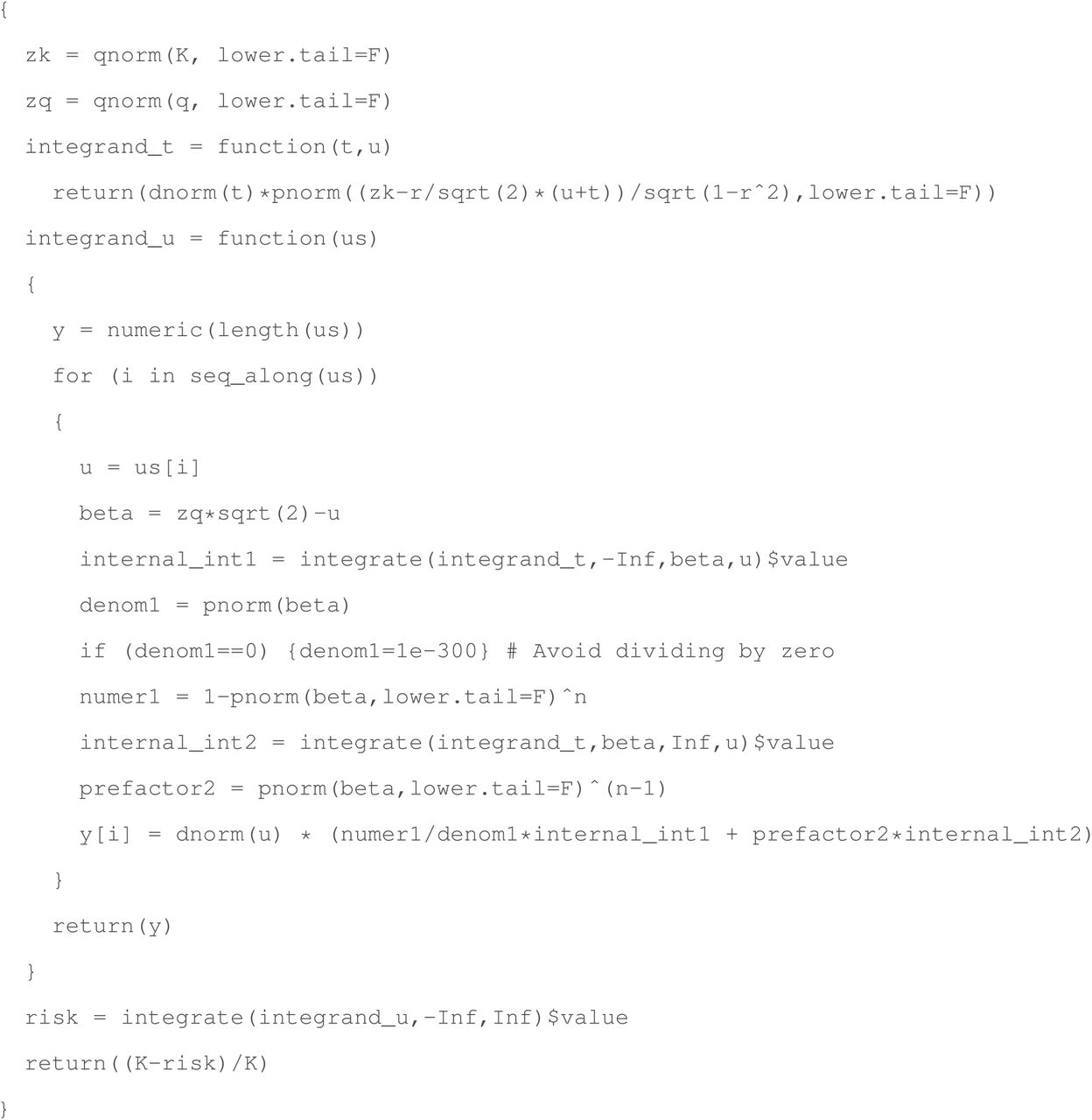
The R code we used to compute the relative risk reduction for the high-risk exclusion (for randomly ascertained parents) strategy is as follows.

The remaining code used to generate the figures of the main text, e.g., when conditioning on the parental scores of disease status, can be found at https://github.com/scarmi/embryo_selection.

Acknowledgements

We thank Gabriel Lázaro-Muñoz and Stacey Pereira for helpful discussions.

Footnotes

• We have added new analyses of risk reduction for polygenic embryo screening when one or both parents are affected with a given disease.